Review

The Role of Instant Centers in Kinematics and Dynamics of Planar Mechanisms: Review of LaMaViP’s Contributions

by
Raffaele Di Gregorio
LaMaViP, Department of Engineering, University of Ferrara, 44122 Ferrara, Italy
Machines 2022, 10(9), 732; https://doi.org/10.3390/machines10090732
Submission received: 30 July 2022 / Revised: 24 August 2022 / Accepted: 25 August 2022 / Published: 26 August 2022
(This article belongs to the Special Issue Advances of Machine Design in Italy 2022)

Abstract

:
Theoretical kinematics and dynamics is one of the research fields where LaMaViP (Laboratory of Mechatronics and Virtual Prototyping) operates, which is the lab leaded by the author at the University of Ferrara. In the last two decades, this research activity at LaMaViP has produced, among others, many novel results that highlight how instant centers’ (ICs) locations condition the kinetostatic and dynamic behaviors of planar mechanisms, and that provide tools suitable for design purposes. This paper reviews/summarizes the tools devised at LaMaViP for PM analysis and synthesis through ICs, and shows that they are a complete set of tools, which make the full description of PMs’ kinematics and dynamics possible, and that the new IC features, identified while setting up these tools, are relevant in machine design.

1. Introduction

Planar mechanisms (PMs) enter in many even spatial machines. That is why ample literature has been devoted to them (e.g., [1,2,3,4,5,6,7,8,9,10,11,12,13,14,15,16]). Instantaneous kinematics and statics of PMs can be fully described [1,2,3] by using instant centers (ICs), which are also relevant in many design problems. For instance, vehicle-suspension design [17], lower-limb prostheses for amputees [18], and Remote Center of Compliance (RCC) systems [19] are only some of these problems.
The use of ICs in PMs’ analysis and synthesis requires the availability of techniques for determining their positions on the motion plane. In single-DOF PMs, the IC positions depend only on the mechanism configuration. Common methods to locate the ICs in single-DOF PMs, are based on the direct application of the Aronhold–Kennedy (AK) theorem. Unfortunately, when the mechanism architecture becomes complex, these methods fail [1,20]. In the literature, the PMs whose ICs cannot be located by directly applying the AK theorem are called “indeterminate” [5].
Graphic methods to locate the ICs of indeterminate PMs have been proposed in the literature [1,5,6,7]. In [1], Klein proposed a graphic trial-and-error method based on the fact that (a) some theorems of projective geometry guarantee the existence of an alternative geometric locus for each secondary IC, not locatable through the AK theorem, and that (b) such a locus can be determined by arbitrarily assuming a number of positions of another secondary IC, for which the AK theorem gives only one straight line, and, then, by coherently determining the positions of the sought-after IC through the AK theorem. So doing, a number of points of the alternative geometric locus are determined, which are sufficient to draw the locus; then, the intersection of the so-determined alternative locus with another locus of the same IC, provided by the AK theorem, gives the correct IC position. In [7], Foster and Pennock proposed another graphic method that can be applied to all the indeterminate PMs. Their work also presents analytical relationships that could be used to formulate an analytical method. Their relationships contain kinematic coefficients whose analytical determination would require the computation of the derivative of the mechanism closure equations. Previously, Yan and Hsu [4] presented another analytic approach, applicable also to multi-DOF PMs, based on a similar principle, which, in practice, requires the solution of the velocity analysis to determine the IC positions. Such analytical approaches, when applied to single-DOF PMs, take no advantage from the fact that the IC positions of these PMs depend only on the mechanism configuration.
In this context, at the Laboratory of Mechatronics and Virtual Prototyping (LaMaViP) [21], an exhaustive analytic technique for the IC-positions’ determination of single-DOF PMs has been conceived which uses only the mechanism-configuration data. Then, in [22], the IC determination in multi-DOF PMs has been addressed and some theoretical results have been proved which make their systematic determination possible.
The availability of analytic techniques for determining the IC positions open to the possibility of devising algorithms that fully describe the instantaneous kinematics of PMs through the ICs. PMs’ singularity analysis is a relevant problem to address when studying PMs’ instantaneous kinematics. Indeed, it is central in the design of parallel PMs (PPMs) since it deeply affects their kinetostatic performances [23]. Singularities are mechanism configurations where mechanism’s instantaneous kinematics becomes indeterminate [24,25,26,27,28]. Hunt [28] identified two special types of mechanism configurations where the instantaneous kinematic behavior is singular: the stationary configurations and the uncertainty configurations. Stationary configurations are mechanism configurations where the rate of a joint variable is instantaneously equal to zero (i.e., the joint is instantaneously inactive which can be alternatively said as follows: “the joint is at a dead center position”). Uncertainty configurations are configurations where the mechanism locally gains extra additional DOFs (transitory mobility). With reference to single-DOF PMs, Hunt [28] highlighted that some of the ICs coincide when the mechanism assumes a stationary configuration; whereas the same ICs fall on particular straight lines when the mechanism assumes an uncertainty configuration. Then, Yan and Wu [29,30] gave a geometric criterion to identify which ICs coincide at a stationary configuration [29] and developed a geometric methodology to generate single-DOF PMs at dead center positions [30].
In this context, at LaMaViP, firstly [31,32], an exhaustive geometric and analytic technique for identifying the singular configurations of single-DOF PMs has been devised which is based on ICs’ positions. Then [22], new theoretical results, which relate ICs positions of multi-DOF PMs with the positions of the same ICs in the single-DOF PMs generated from the multi-DOF one by locking all the actuated joints but one, have been used to set up a novel technique for identifying singularities of multi-DOF PMs.
The IC positions can be also used to compute the velocity (influence) coefficients (VCs) [2,33] of single-DOF PMs and the entries of velocity-coefficient-vectors (VCVs) [34] of multi-DOF PMs, which are indeed VCs of the single-DOF PMs generated from the multi-DOF PM by locking all the generalized coordinates but one. VCs are by definition the ratios between the first-time derivatives (rates) of any two motion variables. In single-DOF PMs, they only depend on the mechanism configuration and enter in both the kinematics [2,33] and statics analyses [32] of these mechanisms. By exploiting this fact with reference to PMs, at LaMaViP, new dynamic formulations [35,36,37,38] have been conceived which fully highlight the role of ICs in PMs’ dynamics.
This paper reviews the tools devised at LaMaViP for PM analysis and synthesis through ICs and shows that they are a complete set of tools, which make the full description of PMs’ kinematics and dynamics possible, and that the new IC features, identified while setting up these tools, are relevant in machine design.
The paper is organized as follows. Section 2, over reminding some background concepts, illustrates the tools devised for ICs’ position determinations and PMs’ singularity analysis. Section 3 illustrates the dynamic formulations. Eventually, Section 4 draws the conclusions.

2. Planar Kinematics Revisited through Instant Centers (ICs)

The instant center, Cji, of the relative (planar) motion between links j and i (Figure 1) is the point of the motion plane that has the same velocity, no matter whether it is considered fixed to one or the other of the two links, whatever be the third link, link k in Figure 1, fixed to the observer that measures its velocity.
Prismatic (P)/revolute (R) pairs and rolling (Cr)/slipping (Cs) contacts are the only kinematic pairs that appear in PMs. P, R and Cr are single-DOF kinematic pairs; whereas, Cs is a two-DOF kinematic pair. In a PM, if links j and i are joined by any of these pairs (see Figure 2), the instant center, Cji, of their relative motion has a known position for the three single-DOF pairs, that is, P, R and Cr (see Figure 2a–c); whereas, it must lie on the common normal at the contact point for Cs contacts (Figure 2d). These four kinematic pairs generate only holonomic and time-independent (scleronomic) constraints [33,34]. Therefore, in PMs, a possible time-dependent (rheonomic) constraint can only be generated by a mobile frame, and, even in this special case, the relative motions between links are scleronomic. Accordingly, in PMs internal motion (i.e., the one with respect to the frame), any motion variable not chosen as generalized coordinate depends only on the chosen generalized coordinates. This fact involves that in l-DOF PMs, the VCs, over depending on the mechanism configuration, depend also on (l − 1) ratios between generalized-coordinate rates (see [22] for details).
In a PM with m links, m(m − 1)/2 relative motions can be identified and as many are the ICs (i.e., one for each relative motion). The relative motion theorems [39] bring the conclusion that only (m − 1) of such motions (e.g., the ones of the mobile links with respect to the frame) are independent (i.e., are sufficient to determine all the remaining ones). Accordingly, determining the positions of (m − 1) ICs is sufficient to solve the velocity analysis of any PM and to fully identify its instantaneous-kinematics features. The ICs whose positions can be determined through a simple inspection of the PM (i.e., the ones related to the single-DOF kinematic pairs) are named “primary” ICs; all the other ICs are named “secondary” ICs [5].
The Aronhold-Kennedy (A-K) theorem states that, in planar motion, the ICs (Cji, Cik, and Cjk in Figure 1) of the three relative motions definable among three rigid bodies (links i, j, and k in Figure 1) must lie on the same line. This condition together with the IC definition brings one to compute the following VCs’ explicit expressions (see Figure 1 and Figure 3).
θ ˙ ji θ ˙ ki = ( C kj C ki ) ( C kj C ji ) C kj C ji 2 ;   s ˙ ji θ ˙ ki = ( C kj C ki ) u ji ;   s ˙ ji s ˙ ri = ( C kj C ki ) u ji ( C kr C ki ) u ri
In Equation (1), a bold capital letter denotes the position vector of the point, the capital letter refers to, in a reference system fixed to the motion plane. The angle θjiki), positive if counterclockwise, identifies the orientation of link j (link k) with respect to link i (see Figure 3a). The unit vector uji (uri) is obtained through a counterclockwise rotation of 90° from the unit vectors tji (tri) (Figure 3b), which gives the positive directions of instantaneous translation, in a relative motion where the IC Cji (Cri) is a point at infinity, and s ˙ ji ( s ˙ ri ) is the signed magnitude of the instantaneous-translation velocity, s ˙ ji t ji ( s ˙ ri t ri ).
Equation (1) and the fact that, in l-DOF PMs, VCs depend on (l − 1) ratios between generalized-coordinate rates bring the conclusion that, in single-DOF PMs, the IC positions depend uniquely on the mechanism configuration; whereas, in l-DOF PMs, they, over depending on the mechanism configuration, depend also on (l − 1) ratios between generalized-coordinate rates [22].

2.1. Instant Center Determination

The analysis of Figure 2 reveals that, in a reference system fixed to PM’s frame, the coordinates of all the primary ICs and, in Cs contacts, the pose parameters of all the normal lines at the contact points depend only on PM’s configuration. Therefore, they can be analytically determined by solving the constraint-equation system once the generalized coordinates of the PM are assigned.

2.1.1. Single-DOF PMs

In single-DOF PMs [21], firstly, the coordinates of all the primary ICs and, in Cs contacts, the pose parameters of all the normal lines at the contact points must be computed as functions of the assigned generalized coordinate. Then, these data must be used together with the AK theorem (Figure 1) for determining the pose parameters of two lines where one secondary IC must lie on. In addition, the equations of the two lines must be written and the system constituted by these two linear equations must be solved to determine the coordinates of the secondary IC that lie on the two lines. Successively, the coordinates of the just-determined secondary IC together with the previously determined data must be used to repeat this algorithm to compute the coordinates of another secondary IC and so on until the coordinates of all the secondary ICs are determined. The central issues to solve for automatically using such a procedure are
(i) the determination of the sequence, hereafter called S0, with which the secondary ICs must be computed;
(ii) the alternative algorithm to use when the determined data are not sufficient to identify two lines where another secondary IC must lie on, which is the case of indeterminate linkages [1,5,6,7,20,21].
If the PM is not indeterminate, issue (i) (i.e., the determination of S0) can be solved by implementing an algorithm easy to deduce from the “circle diagrams” [20,40]. Differently, for indeterminate PMs, the solution of issue (i) is much more cumbersome [1,5,6,7,21] since it is connected to the solution of issue (ii). In [21], both the issues have been solved by using the “table” shown in Figure 4, and a filling procedure for the proposed “table”, which identifies both the sequence S0 in the case of not-indeterminate PMs and the alternative algorithm to use for indeterminate PMs. Such a general technique is illustrated below.
The table to use (Figure 4) for a single-DOF PM with m links and q Cs-contacts has m rows, which one-to-one correspond to the m links, and (m + q) columns with the first m columns corresponding one-to-one to the m links and the last q columns corresponding one-to-one to the q Cs-contacts. In the first m columns, the cells with the row index equal to the column index are black; whereas, all the remaining cells are empty at the beginning of the filling procedure. In these columns, the cell indices identify the IC with the same lower-right indices, that is, the cell (i, j) corresponds to the IC Cij. Since Cij and Cji are the same IC, there are two cells for each IC, which are symmetrically disposed with respect to the diagonal black cells. In the last q columns, only the two cells whose row indices correspond to one or the other of the two links joined by the Cs-contact the column refers to are filled with the symbol “X” and the remaining cells are left empty. In these other columns the two filled cells indicate that the pose parameters of a line, which the IC with indices given by the two row indices of the two filled cells lies on, are known. The central filling rule is that, in the first m column, an empty cell can be filled only when the data necessary to compute the corresponding IC are known. So doing, in the first m column, two filled cells mean that two ICs with one common index (i.e., the one of the column) have known coordinates and identify the pose parameters of a line (i.e., the one passing through the two ICs) on which the IC with indices given by the two row indices of the two filled cells lies. Therefore, the following filling procedure/computation algorithm can be conceived (see Figure 5).
(a)
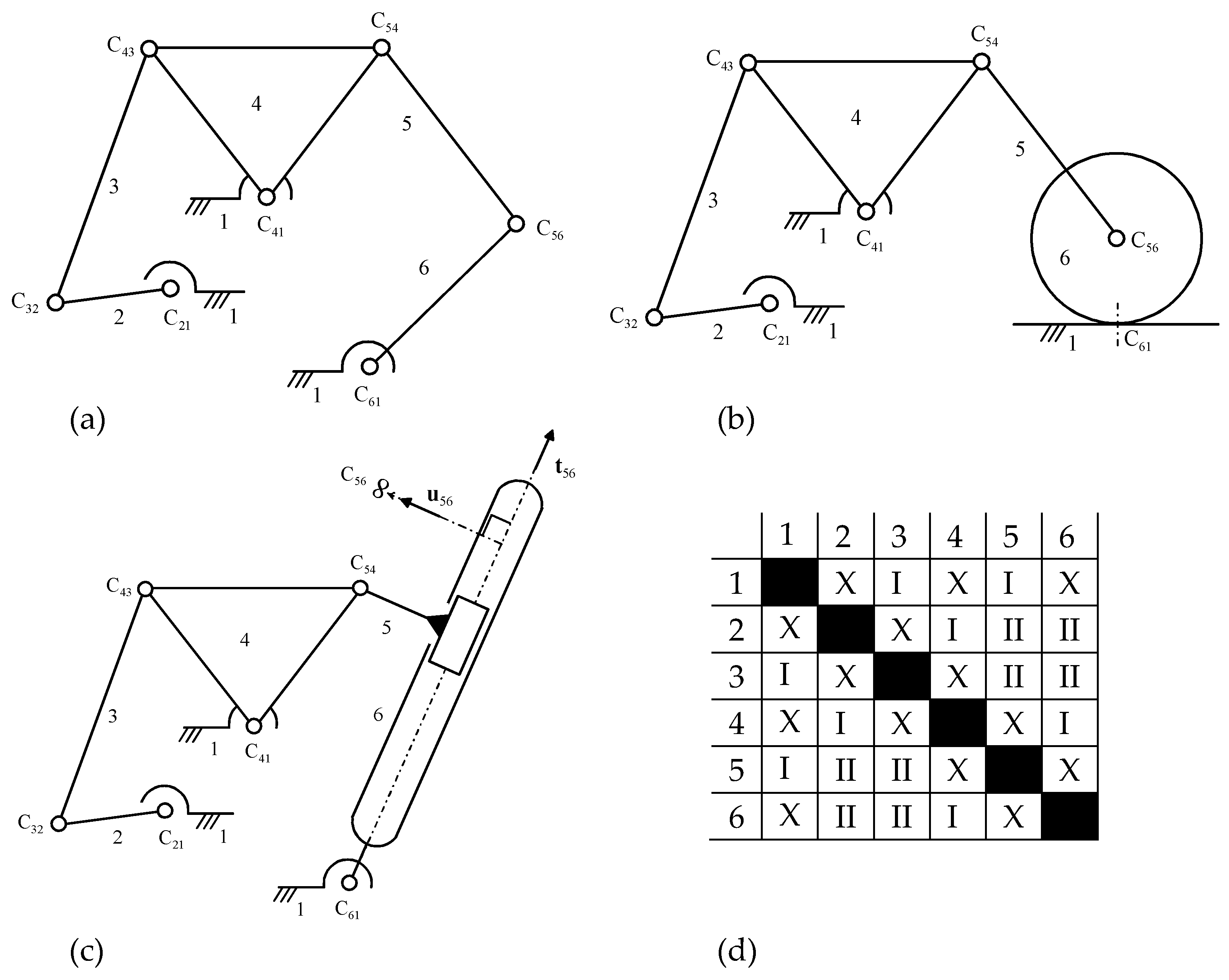
in the first m columns the cells corresponding to the primary ICs are filled with the symbol “X” and the coordinates of these ICs are computed by solving the constraint-equation system;
(b)
the rows with at least two filled cells are selected and compared to identify all the couple of rows that have two filled cells in the same two columns;
(c)
for each couple of rows identified in the previous step, the two linear equations are written which correspond to the lines identified by the two columns with filled cells. The so-obtained system of two linear equations is solved to determine the coordinates of the secondary IC with indices given by the indices of the two rows; then, the corresponding cells are filled with the roman number “I”;
(d)
focusing only on the row couples whose indices correspond to the ones of the still empty cells of the first m columns, the steps (b) and (c) are repeated until either all the cells of the first m columns are filled or at step (b) is not possible to identify any couple of rows (i.e., the mechanism is indeterminate). At each repetition of the steps (b) and (c) the roman number used to fill the cells is increased of one unit (see, Figure 5d);
(e)
if step (d) brings to fill all the cells of the first m columns, the coordinates of all the secondary ICs have been computed and the algorithm is stopped; otherwise (i.e., in the case of indeterminate mechanisms) the following steps are implemented:
(e.1)
focusing only on the row couples whose indices correspond to the ones of the still empty cells of the first m columns, a row couple that has two filled cells in the same column is selected. Moreover, the two cells with indices coincident with the row indices of the selected row couple are filled with the starred roman number “I*”;
(e.2)
the coordinates of the secondary IC, whose indices coincide with the two row indices of the row couple selected in the previous step, are written as the ones of a point lying on the line passing through the two IC identified by the two filled cells located in the above-mentioned same column. That is, a line parameter, say λ, is introduced and the two IC coordinates are explicitly written as linear functions of λ;
(e.3)
focusing only on the row couples whose indices correspond to the ones of the still empty cells of the first m columns, the steps (b) and (c) are repeated by taking into account also the cells filled with “I*” and analytically solving the two-linear-equations system of step (c) still to identify a secondary IC that must lie on three lines. During this step, the cells corresponding to the located ICs are filled with “I*” and the analytic solutions of the above-mentioned equation systems bring to explicitly write the coordinates of these ICs as functions of the parameter λ introduced in the previous step;
(e.4)
the equations of the three lines, which the secondary IC identified in the previous step lies on, are written. Such equations constitute a system of three equations in three unknowns, the two coordinates of the IC and the parameter λ, and the three equations are all linear in the two coordinates of the IC;
(e.5)
the coordinates of the above-mentioned IC are explicitly expressed as functions of λ by solving the first two equations of the system deduced in the previous step. Then, the so-obtained expressions are introduced in the third equation of the same system to obtain one equation in the unique unknown λ;
(e.6)
the equation in λ deduced in step (e.5) is solved and the computed value of λ is back substituted in the explicit expressions of the coordinates of all the ICs deduced in the previous steps to compute their numeric values;
(e.7)
jump to step (d)
It is worth noting that the coordinates of the ICs with the same roman number (see Figure 5d) in the table can be simultaneously computed by using the coordinates of the primary ICs and/or of the secondary ICs with a lower roman number. Accordingly, once the table of Figure 4 has been filled, the roman numbers that appear in it give the sequence S0 with which the secondary-ICs’ positions must be computed.
The table of Figure 4 reveals the following pieces of information about the PM it refers to: the number and the type (binary, ternary, etc.) of links; how many two-DOF and one-DOF pairs (i.e., Cs and primary ICs) there are, and which links they join. Such pieces of information are sufficient to compute the DOF number with the Kutzbach criterion [2]. Since the table does not provide any piece of information about the types of one-DOF pairs the primary ICs refer to, it does not change if a R-pair is replaced by either a P-pair or a Cr contact and vice versa. Consequently, different PMs can be solved together by using the same table. For instance, the table of Figure 5d holds for the three PMs of Figure 5a–c and for many others. Consequently, once the table has been filled for one PM, it gives the IC sequence to use for computing the IC positions of all the PMs that share that table and the computation algorithm is much faster for all the other PMs of this family since the sequence S0 is already known for all of them.
In addition, the proposed table is able to identify both the presence of an over constraint (i.e., a structure or a substructure) and the DOF number of a multi-DOF PM. Indeed, if, during the filling procedure without assuming the position of any secondary IC (i.e., without inserting any starred roman number in the table), either of the following condition is found
(i)
a primary IC must lie on one or more known lines,
(ii)
a still-unknown secondary IC is found which must lie on three or more lines,
particular geometric conditions must be satisfied to make the primary IC lies on the known line(s) (case (i)) or to make the lines have a common intersection (case (ii)), that is, an over constraint is present. In this case, the order of the over constraint is given by the number of lines in case (i) and by the number of lines, which must have a common intersection, minus two in case (ii). Moreover, if, for determining the positions of all the secondary ICs, the positions of a number, say n, of secondary ICs must be assumed on known lines without reaching any over-constraint condition, the PM has n + 1 DOF.

2.1.2. Multi-DOF PMs

In the motion of a generic link j relative to another generic link i (see Figure 3), both belonging to one l-DOF PM, let ωji ( = θ ˙ ji ) and i v O | j denote the signed magnitude, positive if counterclockwise, of the angular velocity and the velocity, measured from link i, of a generic point, O, considered fixed to link j, respectively. The relationship between the 3-tuple (ωji, i v O | j ) and the rates, q ˙ r for r = 1, …, l, of the generalized coordinates, q r for r = 1, …, l, of the l-DOF PM is linear and homogeneous. Such a property makes the superposition principle applicable. In [22], the superposition principle has been exploited to deduce the instantaneous-kinematics relationships that relate an l-DOF PM to the l single-DOF PMs generated from the l-DOF PM by locking all the generalized coordinates but one. Hereafter, for the sake of brevity, the phrase “the r-th single-DOF PM” will mean “the single-DOF PM generated from the l-DOF PM by locking all the generalized coordinates, but the r-th one, that is, with q ˙ k = 0 for any k∈{1, …, l | k ≠ r}.”
Indeed, the application of this principle yields the following relationships (see Figure 6)
ω ji = r = 1 , l ω ji , r
i v O | j = r = 1 , l i v O | j ( r )
where ω ji , r ( i v O | j ( r ) ) is ω ji ( i v O | j ) computed by locking all the generalized coordinates but q r , that is, measured in the r-th single-DOF PM. From now on, (⋅)ji,r will denote the quantity (⋅)ji evaluated in the r-th single-DOF PM. By using complex numbers to represent planar vectors in the Cartesian/Argand reference Oxy (see Figure 6), the following relationships hold (hereafter, a bold letter will denote a planar vector and/or the corresponding complex number according to the context and i = 1 ):
i v O | j = i h ˙ ji d ji
i v O | j ( r ) = i h ˙ ji , r d ji , r
where, with reference to Figure 3 and Figure 6, if ω ji 0 ( ω ji , r 0 ), then h ˙ ji = ω ji = θ ˙ ji ( h ˙ ji , r = ω ji , r = θ ˙ ji , r ) and d ji = C ji ( d ji , r = C ji , r ), else h ˙ ji = s ˙ ji ( h ˙ ji , r = s ˙ ji , r ) and d ji = u ji ( d ji , r = u ji , r ). The introduction of Equations (3a) and (3b) into Equation (2b) transform system (2) as follows
ω ji = r = 1 , l ω ji , r
h ˙ ji d ji = r = 1 , l h ˙ ji , r d ji , r
Equations (4a) and (4b) make it possible to determine the position of Cji in the l-DOF PM once the positions of all the Cji,r for r = 1, …, l (i.e., of the same IC in all the single-DOF PMs generated from the l-DOF PM) are known together with the PM configuration and the generalized-coordinate rates q ˙ r for r = 1, …, l. It is worth stressing that this determination can be conducted even in the case Cji is a point at infinity. This result, deduced in [22], together with the algorithm for the determination of the IC positions in single-DOF PM, presented in [21] and summarized in the previous subsection, makes it possible to determine analytically the IC positions in any PM.
In the case that ω ji 0 and all the Cji,r for r = 1, …, l are finite points of the motion plane, Equation (4) becomes
ω ji = r = 1 , l ω ji , r
ω ji C ji = r = 1 , l ω ji , r C ji , r
which bring the conclusion that, in this case, the following statement is true:
Statement 1.
From a geometric point of view, if the points Cji,r for r = 1, …, l are considered heavy points whose signed weight is ωji,r, Cji is the centroid of these heavy points.
This conclusion makes it possible to employ the simple geometric rules of mass point geometry [41], which, for instance, yield that, in a 2-DOF PM, Cji must lie on the line passing through Cji,1 and Cji,2.

2.2. Singularity Analysis

The instantaneous kinematics (IK) of a mechanism can be described by considering it as an input/output (I/O) device [24,25,26] where the input variables are the actuated-joint rates and the output variables are the ones that uniquely identify the twist of one link chosen as output link. In PMs and, in general, in all the mechanisms with holonomic and time-independent constraints, the analytic relationship (I/O instantaneous relationship) between actuated-joint rates and output-link twist is a linear and homogeneous system where the two coefficient matrices (Jacobians) that multiply the actuated-joint rates and the output-link twist, respectively, depend only on the mechanism configuration. The I/O instantaneous relationship brings one to define two IK problems: the forward IK (FIK) problem and the inverse IK (IIK) problem. The FIK problem is the determination of the output-link twist for assigned actuated-joint rates; vice versa, the IIK problem is the determination of the actuated-joint rates for an assigned output-link twist.
In this context, the mechanism configurations where one or the other or both of the two Jacobians are rank deficient make the FIK or the IIK or both the IK problems undetermined and are the mechanism’s singularities. Accordingly [24], three types of mechanisms’ singularity are identifiable: (I) those that make the IIK problem undetermined (serial singularities), (II) those that make the FIK problem undetermined, (parallel singularities), and (III) those that make both the IIK and the FIK problems undetermined.
At a serial singularity, the output link has a limitation on the possible twists that it can assume, that is, it has a reduction in its instantaneous mobility. Such a condition identifies the workspace boundary. Consequently, serial singularities are configurations where the output link reaches the borders of its motion range, which, in single-DOF PMs, correspond to the extreme values (dead center positions) of one or more variables related to the output-link pose.
At a parallel singularity, the output-link twist can be different from zero even though all the actuated joints are locked, that is, the actuated joints are not able to control the output-link pose any longer and, somehow, the instantaneous mobility of the output link increases. Such singularity can occur inside the output-link workspace and must be avoided during the mechanism motion. In addition, parallel singularities are configurations where at least one of the input links (i.e., those links related to the actuated joints) reaches the borders of its motion range, which, in single-DOF PMs, correspond to the extreme values (dead center positions) of one or more input variables. According to Hunt’s definitions [28], in single-DOF PMs, both serial and parallel singularities are stationary configurations; whereas, type-(III) singularities are uncertainty configurations.
The I/O instantaneous relationship of a single-DOF PM can be written in the following canonical form [31]:
b z ˙ = a q ˙
where q is the generalized coordinate (input variable), z is any possible output variable; whereas, a and b are two coefficients uniquely depending on the PM configuration (i.e., on q). In Equation (6), the input (output) variable q (z) can be either an angle, θji (Figure 3a), related to a relative rotation (Rot) or a linear variable, sji (Figure 3b), related to a relative translation (Tra). Therefore, according to the types of input and output variables, there are only four possible types of Equation (6) (the first (second) acronym refers to the type of input (output) variable): Rot-Rot, Rot-Tra, Tra-Rot, and Tra-Tra. Let “i”, “o”, “f”, and “k” denote the indices of the input link, of the output link, of the reference link that is used to evaluate the rate of the input variable, and of the reference link that is used to evaluate the rate of the output variable, respectively. The positions of the six ICs corresponding to all the possible relative motions among these four links are geometrically related by the AK theorem (Figure 1) as shown in Figure 7. The analytic expressions (see [31] for demonstration and further details) of the coefficients a and b of Equation (6) are reported in Table 1 where Cmn (tmn) with mn∈{if, ok, ik, kf, oi, of} is the complex number that gives the IC position (the unit vector of the positive translation direction (Figure 3b) in the relative motion of link m with respect to link n. Also, as indicated in the note of Table 1, if, for special choices of the indices “i”, “o”, “f”, and “k”, a and b share common factors such factors must be simplified.
Equation (6) reveals that, in single-DOF PMs, a serial (a parallel) singularity occurs at PM configurations for which the coefficient a (the coefficient b) is equal to zero and, accordingly, a type-III singularity occurs when both the coefficients a and b are equal to zero. These conditions and Table 1 yield the geometric conditions to check for identifying single-DOF PMs’ singularities, through the IC positions, reported in Table 2.
In an l-DOF PM, Equations (4a) and (4b) can be exploited to deduce the general I/O instantaneous relationship [22]. Indeed, the replacement of the subscript “ji” with “ok” in Equation (4) transforms them as follows:
ω ok = r = 1 , l ω ok , r
h ˙ ok d ok = r = 1 , l h ˙ ok , r d ok , r
where, for each h ˙ ok , r , the following relationship, deduced from Equation (6), holds
b r h ˙ ok , r = a r q ˙ r r = 1 ,   ,   l
with ar and br that are the coefficients a and b of Table 1 when referred to the r-th single-DOF PM, that is, they are the ones reported in Table 3. It is worth noting that, in Table 3, the values of the indices “i” and “f” depend on the particular r-th single-DOF PM.
The introduction of the analytic expressions of h ˙ ok , r , for r = 1, …, l, obtained from Equation (8) into Equations (7a) and (7b) transforms system (7) as follows
ω ok = r = 1 , l a r b r δ r q ˙ r
h ˙ ok d ok = r = 1 , l a r b r d ok , r q ˙ r
where δr is a binary digit that, if ω ok , r 0 , is equal to 1, else (i.e., if ω ok , r = 0 ) is equal to 0.
System (9), with simple algebraic manipulations, can be put in the following form
( p = 1 , l δ p 0 b p ) ω ok = r = 1 , l a r ( p = 1 , l δ p 0 & p r b p ) δ r q ˙ r
( p = 1 , l b p ) h ˙ ok d ok = r = 1 , l a r ( p = 1 , l p r b p ) d ok , r q ˙ r
which constitute the I/O instantaneous relationship of the l-DOF PM expressed through the ICs. In this relationship, the output-link twist is given through the three-tuple ( ω ok , h ˙ ok d ok ) .
In [22], the analysis of Equation (10) brought this author to demonstrate the following statements and theorems (see [22] for the demonstrations):
Statement 2.
The union of the serial-singularity sets of all the l single-DOF PMs generated from an l-DOF PM is a subset of the set of all the serial singularities of that l-DOF PM.
Theorem 1.
For l ≥ 3 and provided that all the ar and br coefficients are different from zero, a serial singularity of the l-DOF PM occurs if and only if three ICs, Cok,r, are either aligned or all ideal points.
Statement 3.
The set of all the parallel singularities of an l-DOF PM is the union of the l sets of parallel singularities of the single-DOF PMs generated from the l-DOF PM.
Theorem 2.
The coincidence of all the Cok,r, r = 1, …, l, (the Cok,r that are point at infinity are included) identifies a particular parallel singularity where all the br coefficients vanish.
It is worth noting that, since Theorem 1 identifies all the serial singularities that are not serial singularities of any single-DOF PM generated from the l-DOF PM, in two-DOF PMs, the serial-singularity set is the union of the two serial-singularity sets of the two single-DOF PMs generated from the two-DOF PM.
Eventually, both the IIK and the FIK problems are unsolvable (i.e., a type-III singularity occurs) when, at a given configuration, at least one serial-singularity condition together with at least one parallel-singularity condition occur. In particular, if at least one out of the br coefficients together with at least one out of the ar coefficients are equal to zero, a type-(III) singularity will occur. Therefore, the following statement holds [22]:
Statement 4.
The union of the l sets of type-(III) singularities of the single-DOF PMs generated from an l-DOF PM is a subset of the set of all the type-(III) singularities of the l-DOF PM.
The above-reported statements and theorems demonstrate that the singularities of an l-DOF PM can be collected into two classes: (a) configurations that are singular for at least one single-DOF PM generated from the l-DOF PM, and (b) singularities of the l-DOF PM that are not singularities of any single-DOF PM generated from that l-DOF PM (i.e., those identified by Theorem 1). In addition, all the above-listed singularity conditions relate l-DOF PM’s singularities to the IC positions in the single-DOF PMs generated from the l-DOF PM. By exploiting the fact that all the ICs of single-DOF PMs can be analytically/geometrically determined [21] and that the coefficients ar and br together with their vanishing conditions are expressible through the IC of single-DOF PMs (see Table 1, Table 2 and Table 3), an analytic/geometric algorithm for determining l-DOF PM’s singularities has been proposed in [22]. Such an algorithm systematically uses IC positions of single-DOF PMs for identifying the singularities of any PM.
The above-reported singularity conditions are illustrated in Figure 8 through the 3-RRR parallel PM, which is a 3-DOF PM. In this PM (see Figure 8a), links 7 and 0 are chosen as output link (i.e., o = 7) and reference link for all the variables (i.e., k = f = 0); whereas, qr for r = 1, 2, 3 are the actuated-joint (input) variables, and, in the r-th single-DOF PM for r = 1, 2, 3, the input link is link r. So, the three Cok,r for r = 1, 2, 3 are C70,1, C70,2, and C70,3 (see Figure 8). With these choices, the analysis of Figure 8 brings to the following conclusions. The configuration of Figure 8a does not match any singular condition (i.e., it is a non-singular configuration). The configuration of Figure 8b satisfies the singularity condition Coi,1 = Cik,1 (C71,1 = C10,1) of Table 2, that is, it is a serial singularity of the 3-DOF PM, which is also a serial singularity of the 1st single-DOF PM. The configuration of Figure 8c satisfies the geometric condition of Theorem 2 (i.e., the coincidence of all the Cok,r) thus, it is a parallel singularity both of the 3-DOF PM and of all the single-DOF PMs. The configuration of Figure 8d satisfies the geometric condition of Theorem 2 (i.e., the coincidence of all the Cok,r) and the serial-singularity condition Coi,1 = Cik,1 (C71,1 = C10,1) of Table 2, that is, it is a type-(III) singularity.

3. Influence of IC Locations on Planar-Mechanism Dynamics

At LaMaViP, the research on ICs properties, over PMs’ kinematics, addressed also PMs’ dynamics and has brought to provide an exhaustive set of tools for addressing/modelling PMs’ dynamics [35,36,37,38,42]. Since a complete presentation of these tools would require much more room in term of pages than what would be reasonable for a journal paper, the present review was intended to be mainly focused on PMs’ kinematics. Nevertheless, a short summary of the results obtained on PMs’ dynamic is necessary and is presented in this section.

3.1. Single-DOF PMs

The analytic determination of ICs’ positions [21] together with Equation (1) makes the analytic determination of all the VCs in single-DOF PMs possible. The VCs together with their derivative with respect to the generalized coordinate of the single-DOF PM are the only terms necessary to build the dynamic model of a single-DOF PM by using the Eksergian’s equation [43]. This approach has been adopted in [35] to deduce a general dynamic model for single-DOF PMs based on ICs’ positions, which explicitly appear in it. In [35], over the model, the algorithms for systematically solving the two main dynamics problems (i.e., inverse and direct dynamics problems [15]) with this approach have been presented. Then, in [37], by expressing the acceleration of each link’s barycenter through the acceleration of the IC of the relative motion between the same link and the frame, single-DOF PMs’ dynamic models deduced both from Newton-Euler formulation and from D’Alembert’s principle have been built which systematically use ICs’ position. All the dynamic approaches proposed in [35,37] relate single-DOF PMs’ dynamic behavior to ICs’ positions, but are mainly analytic.
From a different point of view, in [38], D’ Alembert’s principle has been revisited and by using a new type of diagram, named “active-load diagram”, a novel geometric and analytic technique for studying single-DOF PMs’ dynamics has been presented which refers PM’s dynamic behavior to ICs’ positions. An active load is, by definition, any internal or external load (force or moment) that provides a non-null virtual work when the mechanism changes its configuration. Accordingly, the active-load diagram of a single-DOF PM is a sketch of the PM, at a given configuration, that also show the active internal loads in the joints and, for each mobile link, all the pieces of information (active loads, Cj1 or uj1, etc.) reported in Figure 9, which are necessary to systematically write the terms appearing in D’ Alembert’s principle. Such a diagram makes it possible to write immediately the dynamic model of the single-DOF PM without any analytic consideration. Indeed, for instance, Figure 10 shows the active-load diagram of a shaper mechanism where the active loads are the external forces F4 and F6, and the moment M12, applied inside the actuated joint, and where, for the sake of simplicity, the hypothesis that inertia forces are negligible is introduced. With reference to Figure 10, from a geometric point of view, the following model of the shaper mechanism can be immediately deduced (here, F 4 = | F 4 | and F 6 = | F 6 | ):
M 12 = F 4 b 4 C 42 C ¯ 21 C 42 C ¯ 41 + F 6 b 6
which gives the following analytic model (here, (xA, yA) are the coordinates of a generic point, A, and (Fj,x, Fj,x) are the components of the force Fj measured in the Cartesian reference C21xy fixed to link 1 (see Figure 10)
M 12 = [ ( x P 4 x C 41 ) F 4 , y ( y P 4 y C 41 ) F 4 , x ] C 42 C ¯ 21 C 42 C ¯ 41 [ ( x C 62 x C 21 ) F 6 , y ( y C 62 y C 21 ) F 6 , x ]
where the ratio C 42 C ¯ 21 C 42 C ¯ 41 is the VC θ ˙ 41 θ ˙ 21 and can be analytically expressed through the first formula of Equation (1).
With reference to Figure 10 and the above-reported relationships, the necessary ICs that are not primary ICs are only two: C31 and C51. Indeed, in this case, since θ31 = θ41, the relationship C 42 C ¯ 21 C 42 C ¯ 41 = C 32 C ¯ 21 C 32 C ¯ 31 holds. Nevertheless, it is worth noting that, when the method is applied to solve only one configuration, it is possible to determine some additional IC (in this case C62) to write also the term associated to the active forces applied to a translating link (link 6) in the form of a moment about an IC. Indeed, in this case, the virtual work of force F6 can be computed as follows:
δ L F 6 = F 6 δ P 6 = δ θ 21 F 6 [ k × ( C 62 C 21 ) ] = k [ ( C 62 C 21 ) × F 6 ] δ θ 21 = F 6 b 6 δ θ 21
where k is the unit vector perpendicular to the motion plane that points toward the reader and F 6 = | F 6 | .
For a single-DOF PM with m links where link 1 is the frame, all the approaches presented in [35,37,38] require the determination of the positions of all the Cj1 for j = 2, …, m (i.e., of (m − 1) ICs). Nevertheless, only a few of these ICs are secondary ICs and really require additional computations. In addition, as it is shown in the case studies presented in [35,38], these additional computations bring to determine VCs that are necessary to write the model; therefore, they are not additional in practice.
In [38], how to write the model in an analytical and systematic form is presented together with the algorithms for solving the two main dynamics problems by using the proposed approach. Eventually, the active-load diagrams, presented in [38], (see Figure 9 and Figure 10, and Equation (11)) immediately reveal that an external force Fj, applied to link j, whose line of action passes through Cj1 (i.e., with bj = 0 (see Figure 9a), if the link rotates, or with vj = uj1 (see Figure 9b), if the link translates) is inactive. That is, it is directly equilibrated by the mechanism structure without requiring the application of a generalized torque in the actuated joint. This result is relevant in PMs’ design since it provides a criterion for reducing the generalized torque in the actuated joint.

3.2. Multi-DOF PMs

At LaMaViP, two formulations [36,42] have been developed which relate multi-DOF PMs’ dynamics to ICs’ position. The first one [36] introduces, for planar motion, rigid-body’s (link’s) configuration space (c-space), which is a three-dimensional space whose coordinates are the “pose coordinates” of the link, that is the two coordinates, say (x, y), of a point fixed to the link plus the slope angle, say θ∈]−π, +π], which identifies the link orientation. Then, it gives the structure of an affine space to the c-space by defining three-dimensional vectors, named planar-pose vectors. Eventually, by using the planar wrench, it formulates the “motion laws” of c-space’s point. Such laws make it possible to study PMs’ dynamics as a number of c-space points that interact one another and stand external planar wrenches. This approach, over providing a coherent, autonomous and self-contained set of tools and laws that model PMs’ kinematics and dynamics, has brought to confirm the above-reported statement 1 and to demonstrate the following new statement on ICs (see [36] for details and examples):
Statement 5.
A planar passive kinematic chain with l-DOF can transmit between links j and i only a force system whose central axis passes through all the instant centers Cji,r for r = 1, …, l.
Statement 5 implies the following corollaries:
(5.a) a single-DOF planar passive kinematic chain can transmit only force systems whose central axis belongs to the pencil of lines passing through the unique Cji;
(5.b) a two-DOF planar passive kinematic chain can transmit only one force with line of action that passes through Cji,1 and Cji,2;
(5.c) an l-DOF planar passive kinematic chain with l ≥ 3 cannot transmit any force system unless the ICs Cji,r for r = 1, …, l are all aligned (i.e., only in particular configurations).
The second formulation [42], by reinterpreting D’ Alembert’s principle, relates the dynamics behavior of an l-DOF PM to the ones of the l single-DOF PMs generated from the l-DOF PM and uses the “active-load diagrams” of these single-DOF PMs to provide a geometric interpretation that fully discloses the role of ICs in multi-DOF PMs’ dynamics. Such diagrams can also be used to write immediately the dynamic model of the l-DOF PM without any analytic consideration. Indeed, for instance, Figure 11a–c show the active-load diagrams of the three single-DOF PMs generated from the 3-RRR parallel PM (Figure 8) with link 7 (mobile platform) loaded by a force system whose resultant force, located on its central axis, is force F7 of Figure 11 and by the generalized torques, τr for r = 1, 2, 3, applied in the actuated joints. With reference to Figure 11, from a geometric point of view, according to this formulation (see [42] for demonstrations) the following model of the 3-RRR parallel PM can be immediately deduced (the signs refer to the configuration of Figure 11 and F 7 = | F 7 | ):
{ τ 1 = F 7 b 7 , 1 θ ˙ 70 , 1 θ ˙ 10 , 1 = F 7 b 7 , 1 C 71 , 1 C ¯ 10 , 1 C 71 , 1 C ¯ 70 , 1 τ 2 = F 7 b 7 , 2 θ ˙ 70 , 2 θ ˙ 20 , 2 = F 7 b 7 , 2 C 72 , 2 C ¯ 20 , 2 C 72 , 2 C ¯ 70 , 2 τ 3 = F 7 b 7 , 3 θ ˙ 70 , 3 θ ˙ 30 , 3 = F 7 b 7 , 3 C 73 , 3 C ¯ 30 , 3 C 73 , 3 C ¯ 70 , 3
Moreover, in [42], how to write the model in an analytical and systematic form is presented together with the algorithms for solving the two main dynamics problems by using the proposed formulation. Eventually, let link 0 be the frame, this formulation immediately reveals (see Figure 11 and Equation (14)) that an external force Fj, applied to link j, whose line of action passes through Cj0,r (i.e., with bj,r = 0 (see Figure 11)) has no effect on the r-th generalized torque τr. This consideration can be further detailed to give a clear graphical idea on how an active load is redistributed among the actuators. Indeed, diagrams such as the ones of Figure 11d where the distances bj,r, of Fj from the ICs Cj0,r, for r = 1, …, l, are drawn all together can be used during design to optimize the load distribution among the actuators.

4. Conclusions

At LaMaViP (Laboratory of Mechatronics and Virtual Prototyping) of Ferrara University, Italy, the research on planar mechanisms’ (PMs) kinematics and dynamics of the last two decades has brought to highlight how the instant-centers’ (ICs) positions can be exploited to identify relevant properties of PMs’ behavior. The results of this research have been summarized/reviewed here to give the reader a guide to use them in PMs’ analysis and design.
In particular, an exhaustive technique for analytically determining IC positions, even for indeterminate PMs, has been obtained and the relationship between one IC in a multi-DOF PM and the same IC in the single-DOF PMs generated from that multi-DOF PM has been identified.
The geometric conditions that ICs’ positions satisfy when a PMs is at a singular configuration have been exhaustively enumerated and analytic techniques that exploit such conditions to implement PMs’ singularity analysis have been developed.
The role that ICs’ positions play to determine PMs’ dynamic behavior has been fully disclosed and PM-dynamics formulations that explicitly contain ICs’ positions have been developed.
Such findings provide a complete set of tools that can be easily used for PMs’ analysis and design.

Funding

This research was funded by University of Ferrara (UNIFE), FAR2020 and developed at the Laboratory of Mechatronics and Virtual Prototyping (LaMaViP), Department of Engineering, UNIFE.

Institutional Review Board Statement

Not applicable.

Informed Consent Statement

Not applicable.

Data Availability Statement

Not applicable.

Conflicts of Interest

The authors declare no conflict of interest. The funders had no role in the design of the study; in the collection, analyses, or interpretation of data; in the writing of the manuscript, or in the decision to publish the results.

References

  1. Klein, A.W. Kinematics of Machinery; McGraw-Hill Book Company, Inc.: New York, NY, USA, 1917. [Google Scholar]
  2. Paul, B. Kinematics and Dynamics of Planar Machinery; Prentice-Hall, Inc.: Englewood Cliffs, NJ, USA, 1987. [Google Scholar]
  3. Gans, R.F. Analytical Kinematics: Analysis and Synthesis of Planar Mechanisms; Butterworth-Heinemann Inc.: Boston, MA, USA, 1991. [Google Scholar]
  4. Yan, H.-S.; Hsu, M.-H. An analytical method for locating instantaneous velocity centers. In Proceedings of the 22nd ASME Biennial Mechanisms Conference, Scottsdale, AZ, USA, 13–16 September 1992; Volume 47, pp. 353–359. [Google Scholar]
  5. Foster, D.E.; Pennock, G.R. A Graphical Method to Find the Secondary Instantaneous Centers of Zero Velocity for the Double Butterfly Linkage. ASME J. Mech. Des. 2003, 125, 268–274. [Google Scholar] [CrossRef]
  6. Pennock, G.R.; Kinzel, E.C. Path curvature of the single flier eight-bar linkage. ASME J. Mech. Des. 2004, 126, 470–477. [Google Scholar] [CrossRef]
  7. Foster, D.E.; Pennock, G.R. Graphical methods to locate the secondary instantaneous centers of single-degree-of-freedom indeterminate linkages. ASME J. Mech. Des. 2005, 127, 249–256. [Google Scholar] [CrossRef]
  8. Butcher, E.A.; Hartman, C. Efficient enumeration and hierarchical classification of planar simple-jointed kinematic chains: Application to 12- and 14-bar single degree-of-freedom chains. Mech. Mach. Theory 2005, 40, 1030–1050. [Google Scholar] [CrossRef]
  9. Cardona, A.; Pucheta, M. An automated method for type synthesis of planar linkages based on a constrained subgraph isomorphism detection. Multibody Syst. Dyn. 2007, 18, 233–258. [Google Scholar]
  10. Murray, A.P.; Schmiedeler, J.P.; Korte, B.M. Kinematic Synthesis of Planar, Shape-Changing Rigid-Body Mechanisms. ASME J. Mech. Des. 2008, 130, 032302. [Google Scholar] [CrossRef]
  11. Kong, X.; Huang, C. Type synthesis of single-DOF single-loop mechanisms with two operation modes. In Proceedings of the ASME/IFToMM International Conference on Reconfigurable Mechanisms and Robots, ReMAR 2009, London, UK, 22–24 June 2009; pp. 136–141. [Google Scholar]
  12. Wolbrecht, E.T.; Reinkensmeyer, D.J.; Perez-Gracia, A. Single degree-of-freedom exoskeleton mechanism design for finger rehabilitation. In Proceedings of the 2011 IEEE International Conference on Rehabilitation Robotics, Zurich, Switzerland, 29 June–1 July 2011; pp. 1–6. [Google Scholar] [CrossRef]
  13. Wang, J.; Ting, K.-L.; Zhao, D. Equivalent Linkages and Dead Center Positions of Planar Single-Degree-of-Freedom Complex Linkages. ASME J. Mech. Robot. 2015, 7, 044501. [Google Scholar] [CrossRef]
  14. St-Onge, D.; Gosselin, C.M. Synthesis and Design of a One Degree-of-Freedom Planar Deployable Mechanism with a Large Expansion Ratio. ASME J. Mech. Robot. 2016, 8, 021025. [Google Scholar] [CrossRef]
  15. Nikravesh, P.E. Planar Multibody Dynamics: Formulation, Programming, and Applications; CRC Press: Boca Raton, FL, USA, 2008. [Google Scholar]
  16. Flores, P.; Seabra, E. Dynamics of Planar Multibody Systems; VDM: Saarbrucken, Germany, 2010. [Google Scholar]
  17. Dixon, J.C. Suspension Geometry and Computation; John Wiley & Sons Ltd.: Chichester, UK, 2009. [Google Scholar]
  18. Windrich, M.; Grimmer, M.; Christ, O.; Rinderknecht, S.; Beckerle, P. Active lower limb prosthetics: A systematic review of design issues and solutions. Biomed. Eng. Online 2016, 15, 5–19. [Google Scholar] [CrossRef]
  19. Watson, P.C. Remote Center Compliant System. U.S. Patent US4098001, 4 July 1978. [Google Scholar]
  20. Kumar Mallik, A.; Ghosh, A.; Dittirich, G. Kinematic Analysis and Synthesis of Mechanisms; CRC: Boca Raton, FL, USA, 1994. [Google Scholar]
  21. Di Gregorio, R. An Algorithm for Analytically Calculating the Positions of the Secondary Instant Centers of Indeterminate Linkages. ASME J. Mech. Des. 2008, 130, 042303. [Google Scholar] [CrossRef]
  22. Di Gregorio, R. A novel method for the singularity analysis of planar mechanisms with more than one degree of freedom. Mech. Mach. Theory 2009, 44, 83–102. [Google Scholar] [CrossRef]
  23. Gosselin, C.; Angeles, J. A Global Performance Index for the Kinematic Optimization of Robotic Manipulators. ASME J. Mech. Des. 1991, 113, 220–226. [Google Scholar] [CrossRef]
  24. Gosselin, C.M.; Angeles, J. Singularity analysis of closed-loop kinematic chains. IEEE Trans. Robot. Autom. 1990, 6, 281–290. [Google Scholar] [CrossRef]
  25. Ma, O.; Angeles, J. Architecture singularities of platform manipulators. In Proceedings of the 1991 IEEE International Conference on Robotics and Automation (ICRA1991), Sacramento, CA, USA, 9–11 April 1991; pp. 1542–1547. [Google Scholar]
  26. Zlatanov, D.; Fenton, R.G.; Benhabib, B. A Unifying Framework for Classification and Interpretation of Mechanism Singularities. ASME J. Mech. Des. 1995, 117, 566–572. [Google Scholar] [CrossRef]
  27. Bonev, I.A.; Zlatanov, D.; Gosselin, C.M.M. Singularity Analysis of 3-DOF Planar Parallel Mechanisms via Screw Theory. ASME J. Mech. Des. 2003, 125, 573–581. [Google Scholar] [CrossRef]
  28. Hunt, K.H. Kinematic Geometry of Mechanisms; Oxford University Press: Oxford, UK, 1978; ISBN 0-19-856124-5. [Google Scholar]
  29. Yan, H.-S.; Wu, L.-I. The stationary configurations of planar six-bar kinematic chains. Mech. Mach. Theory 1988, 23, 287–293. [Google Scholar] [CrossRef]
  30. Yan, H.-S.; Wu, L.-I. On the dead-center positions of planar linkage mechanisms. ASME J. Mech. Transm. Automat. Des. 1989, 111, 40–46. [Google Scholar] [CrossRef]
  31. Di Gregorio, R. A novel geometric and analytic technique for the singularity analysis of one-dof planar mechanisms. Mech. Mach. Theory 2007, 42, 1462–1483. [Google Scholar] [CrossRef]
  32. Simionescu, P.A.; Talpasanu, I.; Di Gregorio, R. Instant-Center Based Force Transmissivity and Singularity Analysis of Planar Linkages. ASME J. Mech. Robot. 2010, 2, 021011. [Google Scholar] [CrossRef]
  33. Di Gregorio, R. Systematic use of velocity and acceleration coefficients in the kinematic analysis of single-DOF planar mechanisms. Mech. Mach. Theory 2019, 139, 310–328. [Google Scholar] [CrossRef]
  34. Di Gregorio, R. Kinematic analysis of multi-DOF planar mechanisms via velocity-coefficient vectors and acceleration-coefficient Jacobians. Mech. Mach. Theory 2019, 142, 103617. [Google Scholar] [CrossRef]
  35. Di Gregorio, R. A Novel Dynamic Model for Single Degree-of-Freedom Planar Mechanisms Based on Instant Centers. ASME J. Mech. Robot. 2016, 8, 011013. [Google Scholar] [CrossRef]
  36. Di Gregorio, R. Kinematics and dynamics of planar mechanisms reinterpreted in rigid-body’s configuration space. Meccanica 2015, 51, 993–1005. [Google Scholar] [CrossRef]
  37. Di Gregorio, R. On the Use of Instant Centers to Build Dynamic Models of Single-dof Planar Mechanisms. In Advances in Robot Kinematics 2018 (ARK2018), Proceedings of the 16th International Symposium on Advances in Robot Kinematics, Bologna, Italy, 1–5 July 2018; Lenarcic, J., Parenti-Castelli, V., Eds.; Springer: Cham, Switzerland, 2018; Volume 8, pp. 242–249. [Google Scholar]
  38. Di Gregorio, R. A geometric and analytic technique for studying single-DOF planar mechanisms’ dynamics. Mech. Mach. Theory 2021, 168, 104609. [Google Scholar] [CrossRef]
  39. Ardema, M.D. Newton-Euler Dynamics; Springer: New York, NY, USA, 2005. [Google Scholar]
  40. Barton, L.O. Mechanism Analysis: Simplified Graphical and Analytical Techniques; Marcel Dekker Inc.: New York, NY, USA, 1993; ISBN 9780429102493. [Google Scholar]
  41. Coxeter, H.S.M. Introduction to Geometry, 2nd ed.; John Wiley & Sons Inc.: New York, NY, USA, 1969; ISBN 9780471504580. [Google Scholar]
  42. Di Gregorio, R. A geometric and analytic technique for studying multi-DOF planar mechanisms’ dynamics. Mech. Mach. Theory 2022, 176, 104975. [Google Scholar] [CrossRef]
  43. Eksergian, R. Dynamical Analysis of Machines. Ph.D. Thesis, Clark University, Worcester, MA, USA, 1928. [Google Scholar]
Figure 1. Diagram of the Aronhold-Kennedy theorem.
Machines 10 00732 g001
Figure 2. Position of the IC, Cji, in the four kinematic pairs that can appear in PMs: (a) revolute pair, (b) prismatic pair, (c) rolling contact, and (d) slipping contact.
Machines 10 00732 g002
Figure 3. Relative (planar) motion between any two links, denoted j and i: (a) instantaneous rotation (the IC Cji is a finite point), (b) instantaneous translation along the direction of the unit vector tji (the IC Cji is the point at infinity the unit vector uji points to).
Machines 10 00732 g003
Figure 4. Table proposed in [21] to determine all the secondary ICs of a single-DOF PM with m links and q Cs-contacts. The first row (column) just contains the column (row) index and it is just a heading row (column).
Machines 10 00732 g004
Figure 5. The three PMs (ac) share the same table (d).
Machines 10 00732 g005
Figure 6. Instantaneous relative motion between two links, j and i, of an l-DOF PM (Cji,r denotes the IC of this relative motion in the r-th single-DOF PM) when (a) Cji,r is a finite point (rotation around Cji,r), and (b) Cji,r is a point at infinity located by the unit vector uji,r (translation with the direction of the unit vector tji,r).
Machines 10 00732 g006
Figure 7. Geometric relationship among the positions of the six ICs corresponding to all the possible relative motions among the links i, o, f, and k.
Machines 10 00732 g007
Figure 8. The 3-RRR parallel PM: (a) non-singular configuration, (b) serial singularity that is also a serial singularity of the 1st single-DOF PM (i.e., the one obtained by locking q2 and q3), (c) parallel singularity that satisfy Theorem 2, (d) type-(III) singularity that satisfies Theorem 2 and, simultaneously, is a serial singularity of the 1st single-DOF PM.
Machines 10 00732 g008
Figure 9. Active-load diagram of the j-th link of a single-DOF PM (link 1 is the frame and O1×1y1 is a Cartesian reference fixed to link 1; Fj (Mj) is a generic external force (moment) applied to link j; mj, Gj, and Ij are mass, barycenter and mass moment of inertia about Gj of the j-th link, respectively): (a) instantaneous rotation of the j-th link, (b) instantaneous translation of the j-th link.
Machines 10 00732 g009
Figure 10. Active-load diagram of the shaper mechanism.
Machines 10 00732 g010
Figure 11. Active-load diagrams of the three single-DOF PMs generated from the 3-RRR parallel PM: (a) r = 1 (i.e., q2 and q3 are locked), (b) r = 2 (i.e., q1 and q3 are locked), (c) r = 3 (i.e., q1 and q2 are locked), (d) extract of the previous diagrams that is useful to visualize how an active force is redistributed among the actuators.
Machines 10 00732 g011
Table 1. Analytic expressions of the coefficients a and b appearing in the I/O instantaneous relationships (Equation (6)) of single-DOF PMs deduced in [31] (Cmn (tmn) with mn∈{if, ok, ik, kf, oi, of} is the complex number that gives the IC position (the unit vector of the positive-translation direction (Figure 3b) of the relative motion of link m with respect to link n).
Input-Output q ˙ z ˙ a (*)b (*)
Rot-Rot ω if = θ ˙ if ω ok = θ ˙ ok (CofCif)(CoiCik)(CokCik)(CoiCof)
Rot-Tra ω if = θ ˙ if s ˙ ok (CofCif)(CoiCik)i tok (CoiCof)
Tra-Rot s ˙ if ω ok = θ ˙ ok i tif (CoiCik)(CokCik)(CofCoi)
Tra-Tra s ˙ if s ˙ ok i tif (CoiCik)i tok (CofCoi)
(*) If, for special choices of the indices ‘‘i”, ‘‘o”, ‘‘f”, and ‘‘k”, a and b share common factors such factors must be simplified.
Table 2. Geometric conditions on the IC positions that identify the singularities of single-DOF PMs.
Input-Output q ˙ z ˙ a = 0
(Serial Singularity)
b = 0
(Parallel Singularity)
Rot-Rot ω if = θ ˙ if ω ok = θ ˙ ok Cof = Cif or Coi = CikCok = Cik or Coi = Cof
Rot-Tra ω if = θ ˙ if s ˙ ok Cof = Cif or Coi = CikCoi = Cof
Tra-Rot s ˙ if ω ok = θ ˙ ok Coi = CikCok = Cik or Cof = Coi
Tra-Tra s ˙ if s ˙ ok Coi = CikCof = Coi
Table 3. Analytic expressions of the coefficients ar and br appearing in the I/O instantaneous relationship (Equation (8)) of the r-th single-DOF PM (Cmn,r (tmn,r) with mn∈{if, ok, ik, kf, oi, of} is the complex number that gives the IC position (the unit vector of the positive-translation direction (Figure 3b) of the relative motion of link m with respect to link n in the r-th single-DOF PM).
Input-Output q ˙ r h ˙ ok , r ar (*)br (*)
Rot-Rot ω if , r = θ ˙ if , r ω ok , r = θ ˙ ok , r (Cof,rCif,r)(Coi,rCik,r)(Cok,rCik,r)(Coi,rCof,r)
Rot-Tra ω if , r = θ ˙ if , r s ˙ ok , r (Cof,rCif,r)(Coi,rCik,r)i tok,r (Coi,rCof,r)
Tra-Rot s ˙ if , r ω ok , r = θ ˙ ok , r i tif,r (Coi,rCik,r)(Cok,rCik,r)(Cof,rCoi,r)
Tra-Tra s ˙ if , r s ˙ ok , r i tif,r (Coi,rCik,r)i tok,r (Cof,rCoi,r)
(*) If, for special choices of the indices ‘‘i”, ‘‘o”, ‘‘f”, and ‘‘k”, ar and br share common factors such factors must be simplified.
Publisher’s Note: MDPI stays neutral with regard to jurisdictional claims in published maps and institutional affiliations.

