
Suppressing Quadrature Error and Harmonics in Resolver Signals via Disturbance-Compensated PLL


Abstract
:1. Introduction
2. Effect of Non-Ideal Factors on RDC
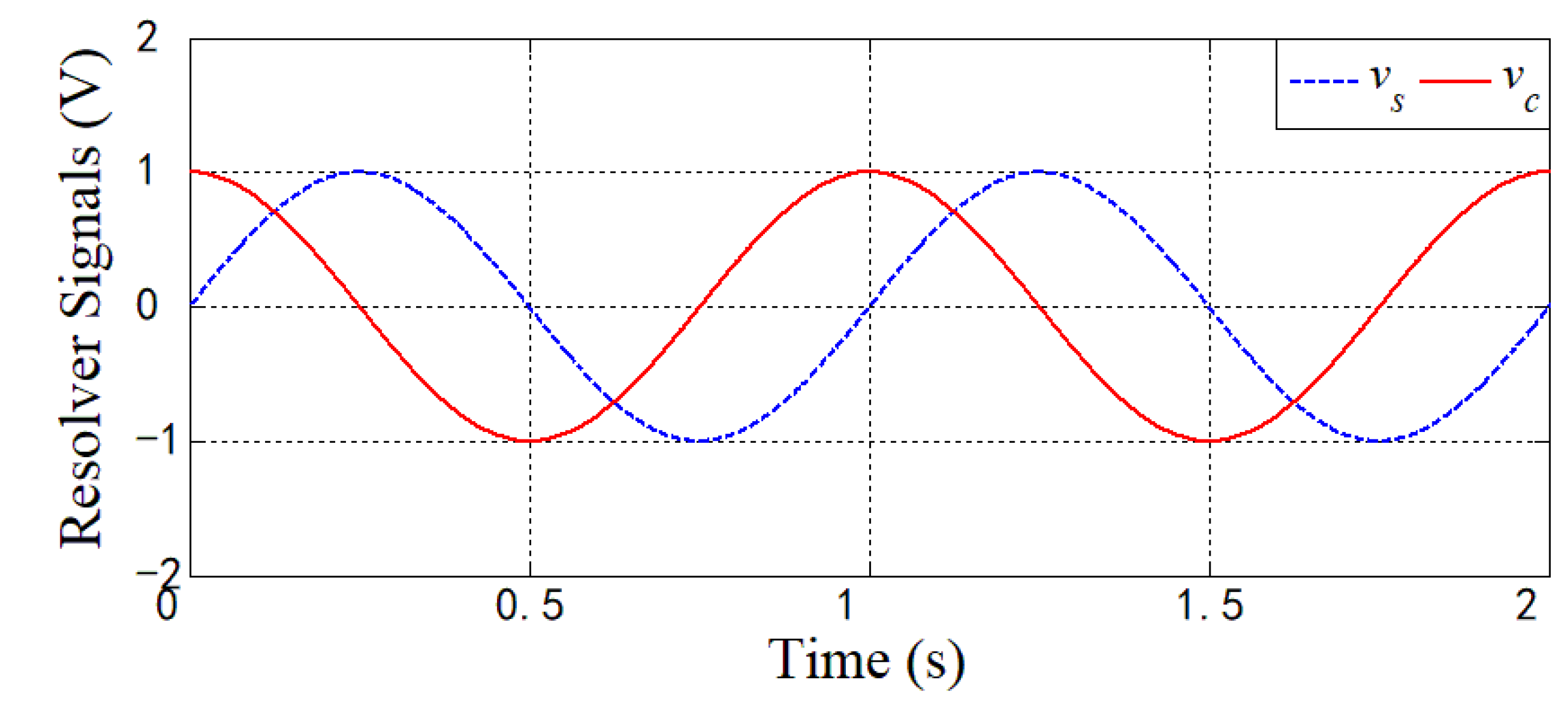
2.1. RDC Principles
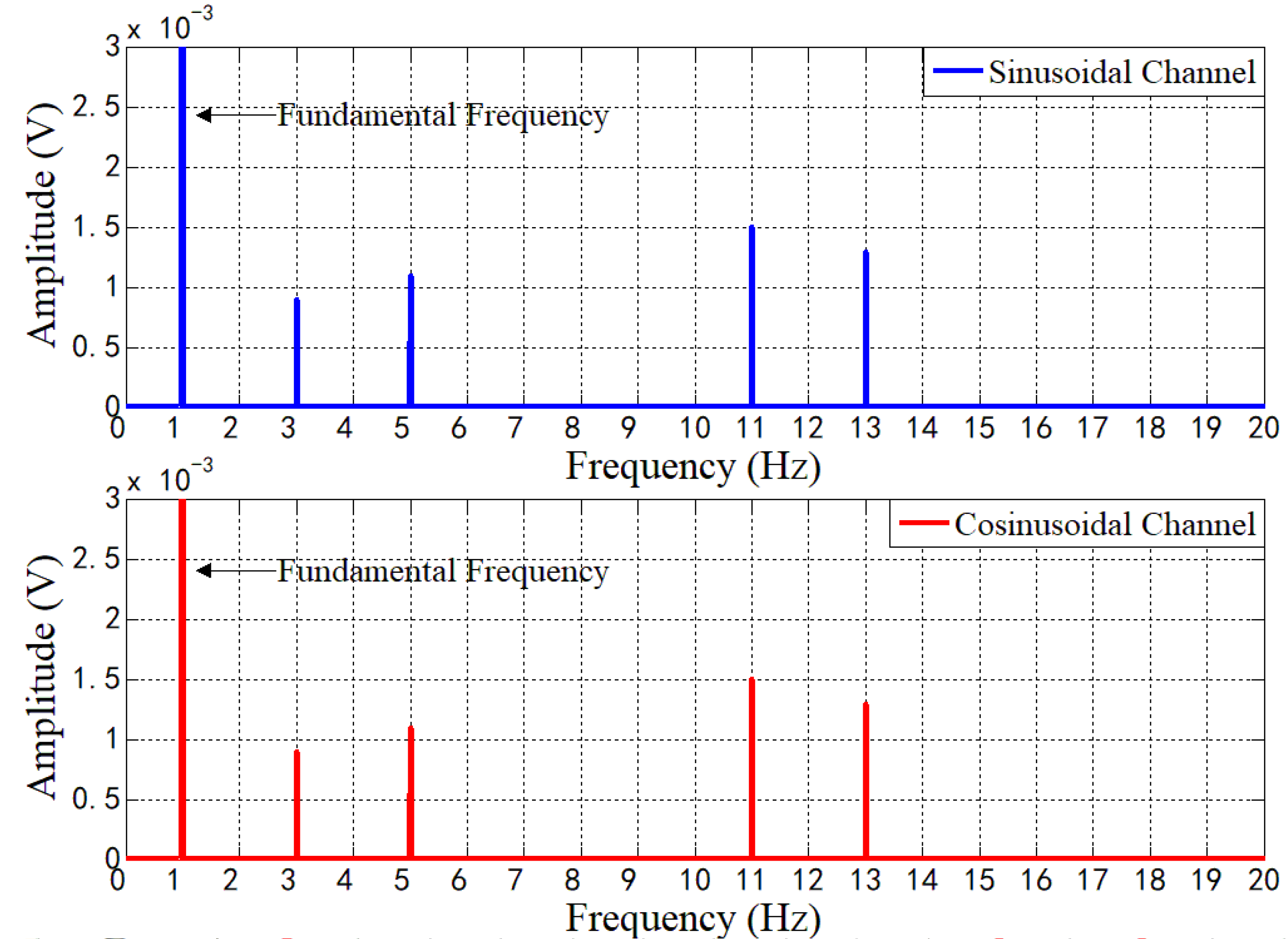
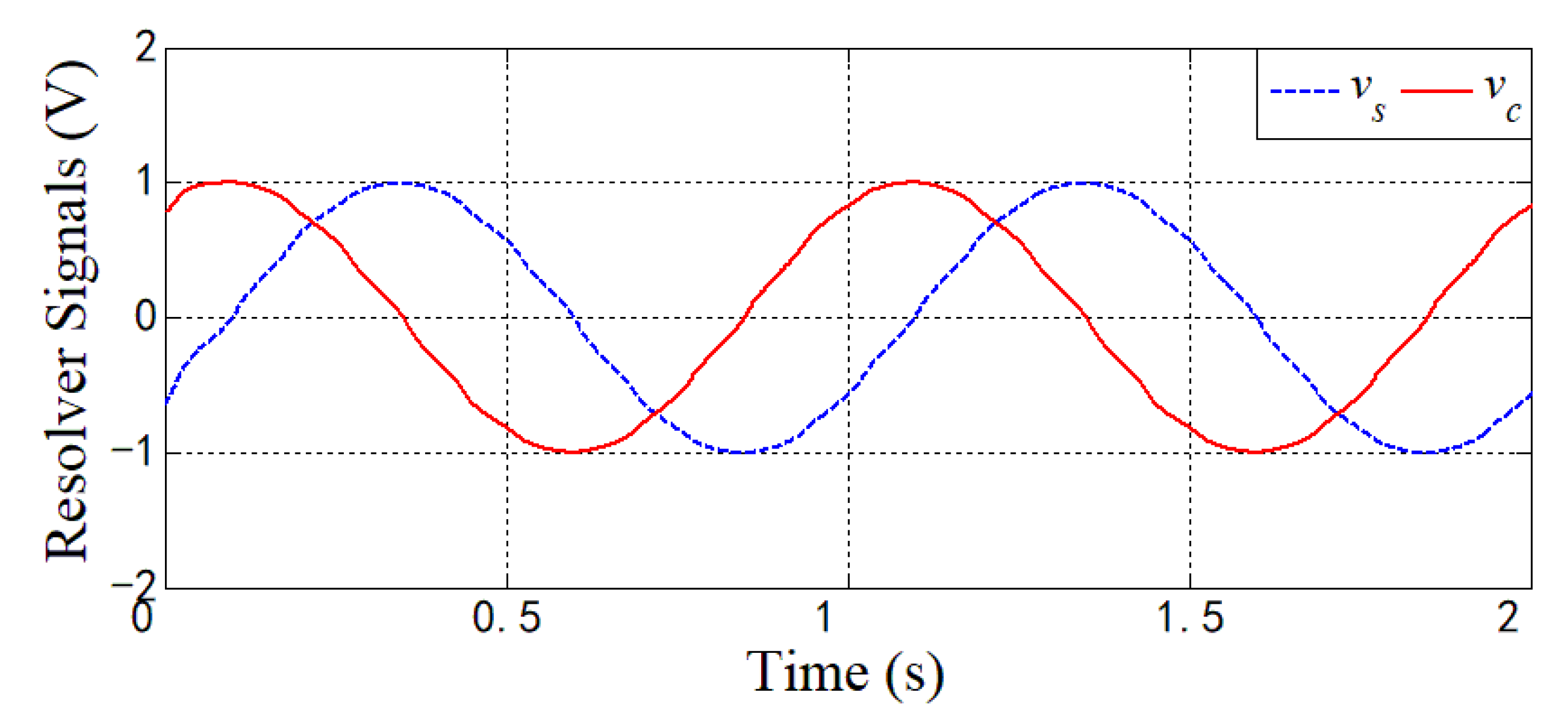
2.2. Analysis of Quadrature Error and Harmonics Effect on PLL
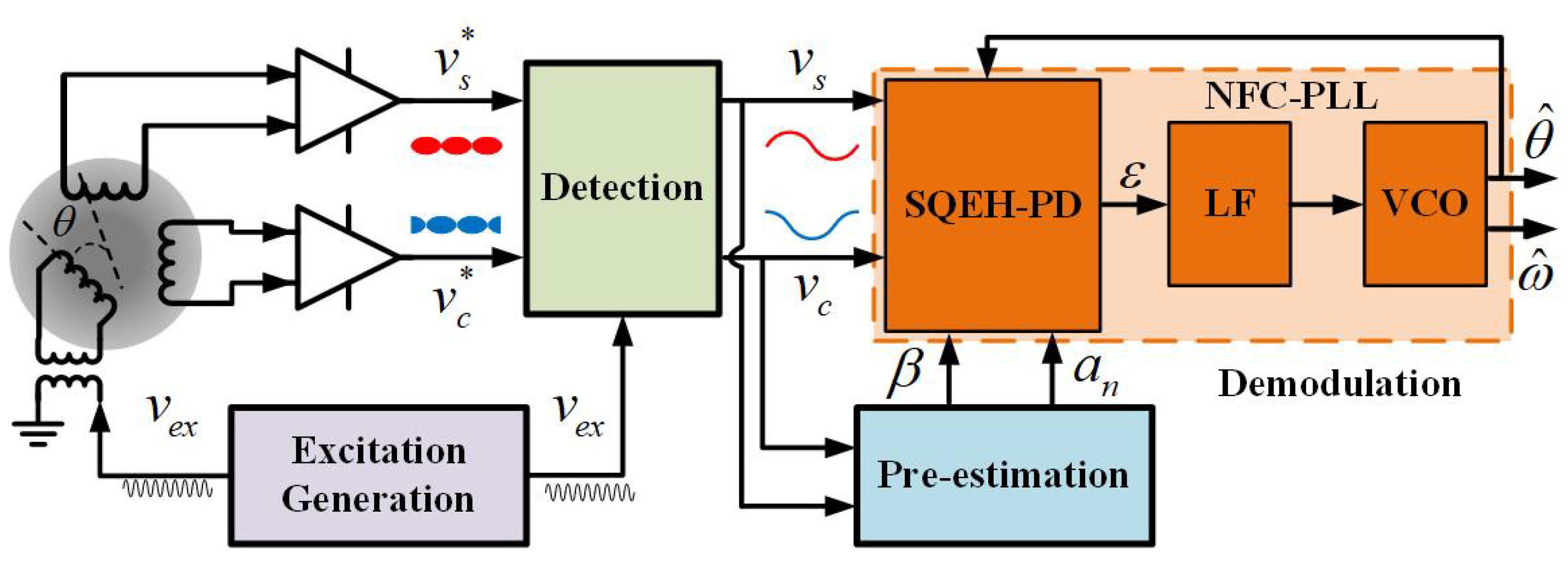
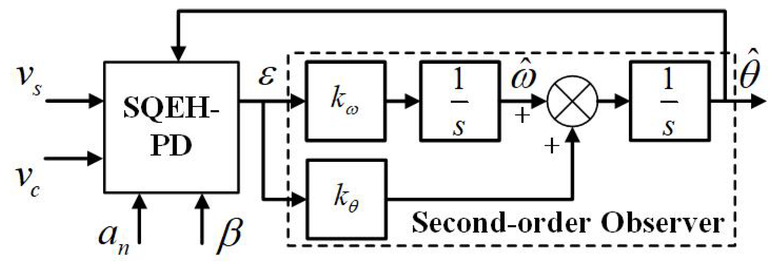
3. Disturbance-Compensated PLL
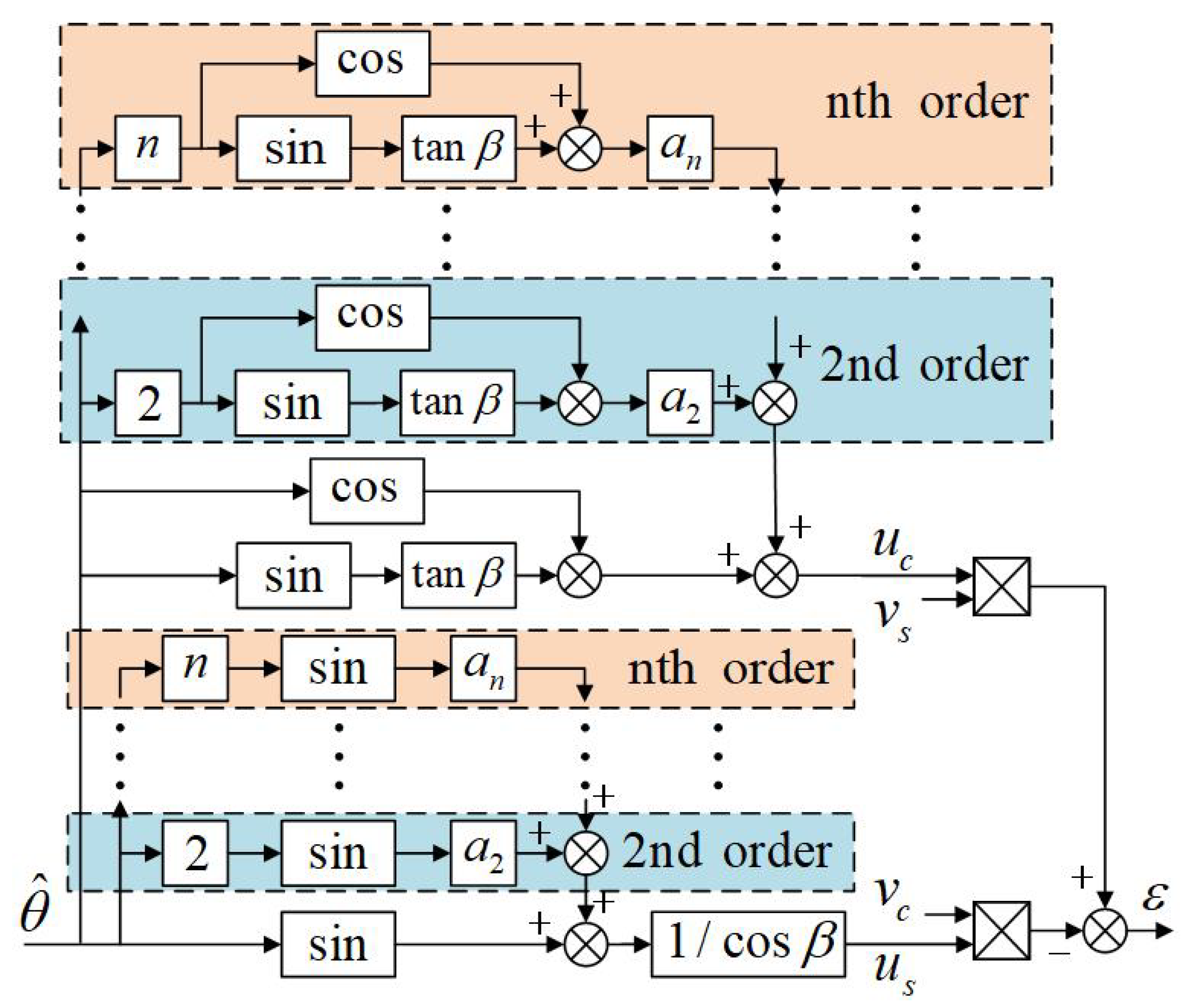
3.1. Phase Detector for Suppressing Quadrature Error and Harmonics
3.2. Second-Order Observer
4. Simulation and Experimental Results
4.1. Simulation Results
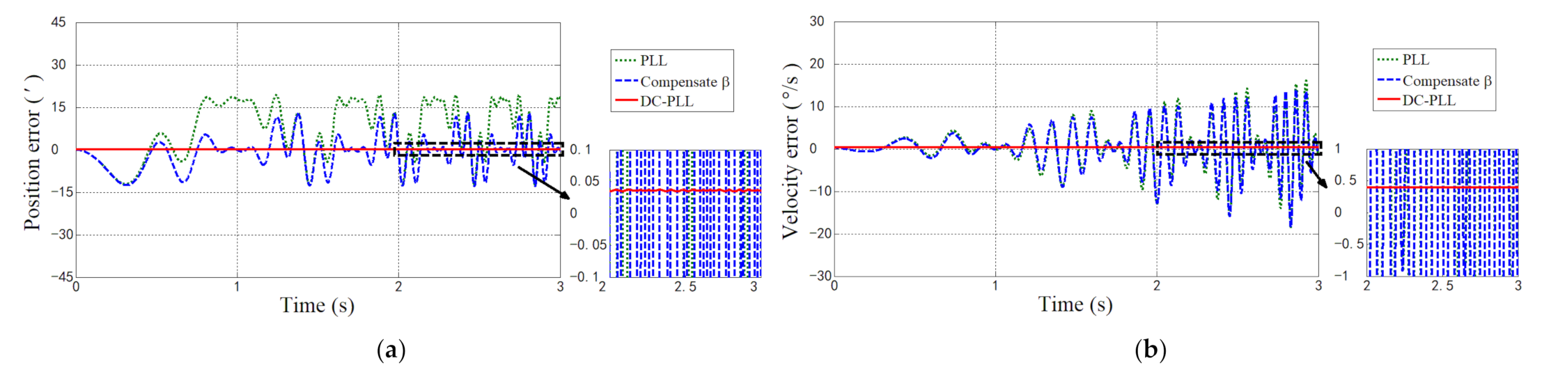
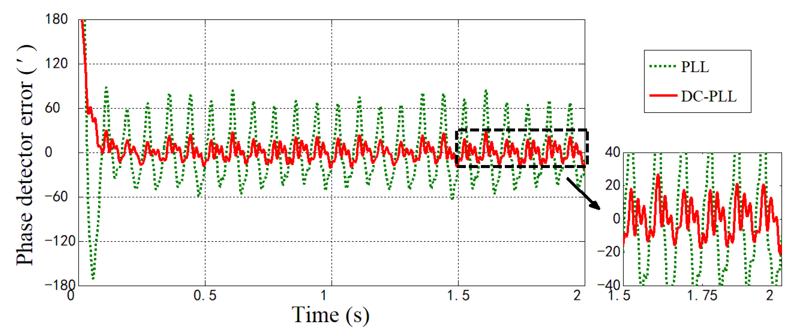
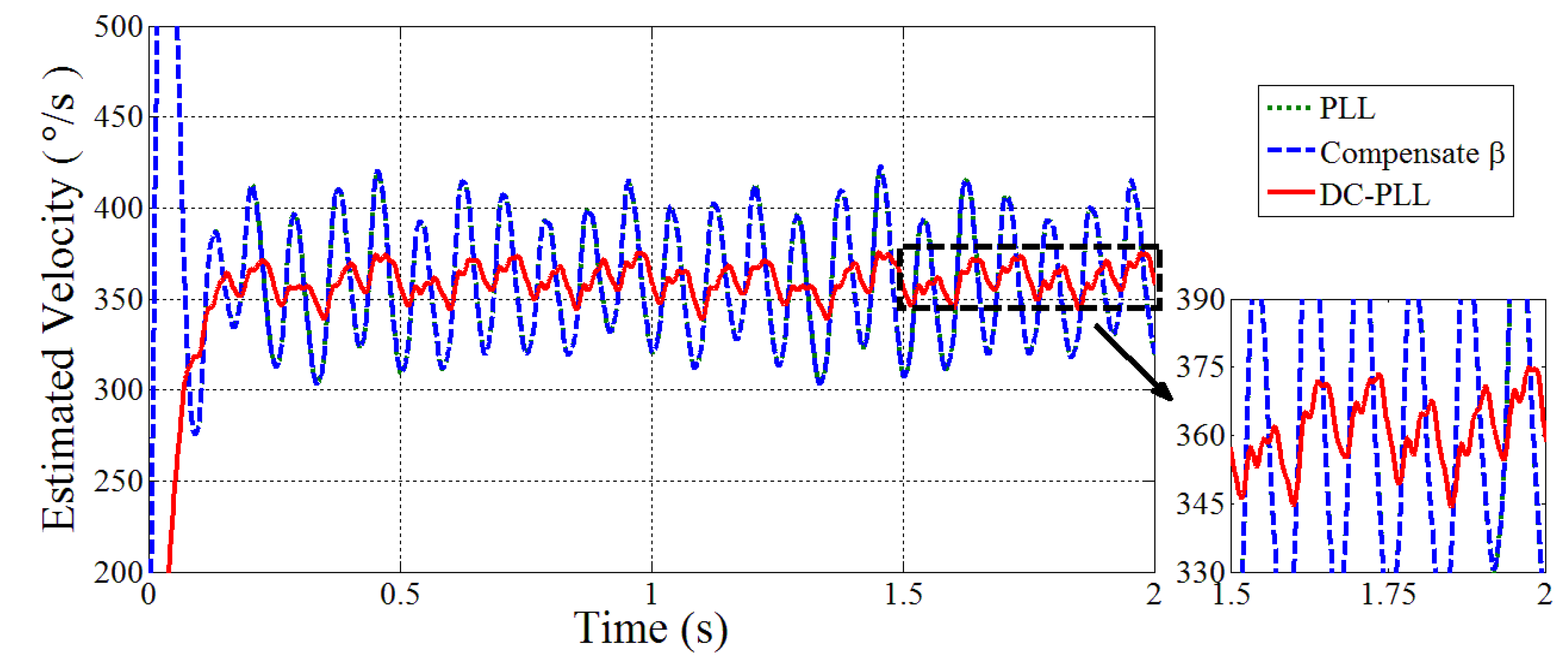
4.1.1. Case 1: Constant Velocity ()
4.1.2. Case 2: Constant Acceleration ()
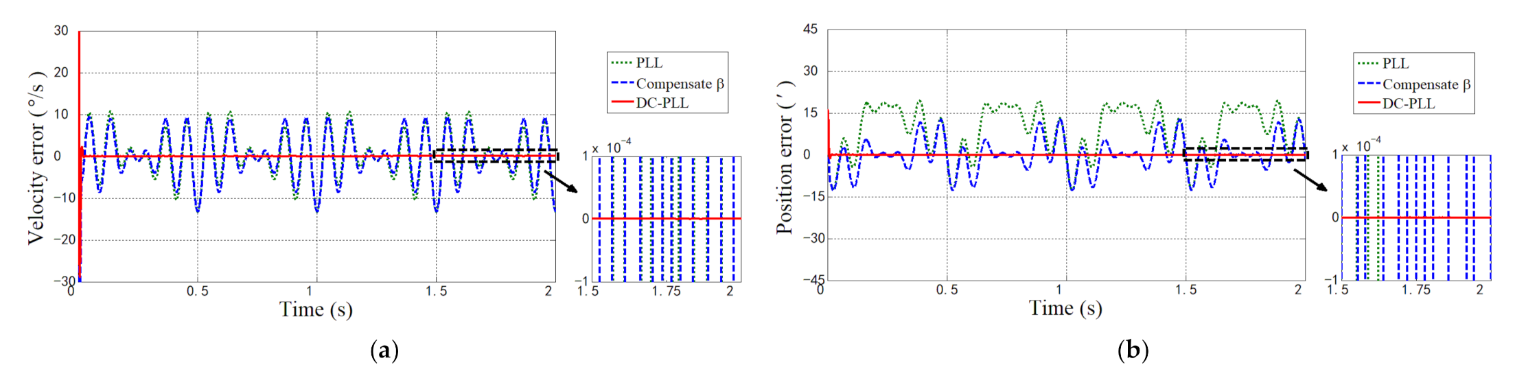
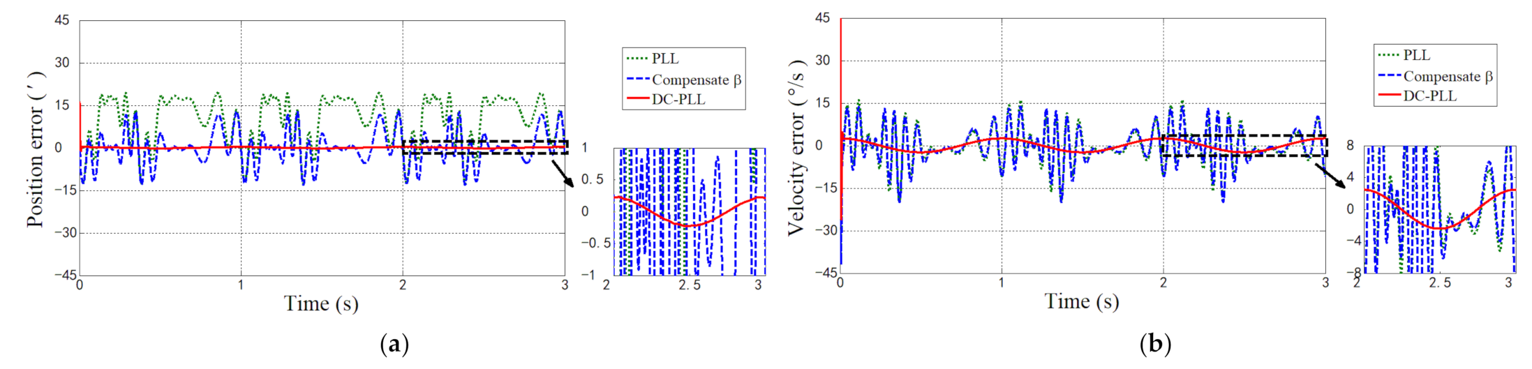
4.1.3. Case 3: Sinusoidal Velocity ()
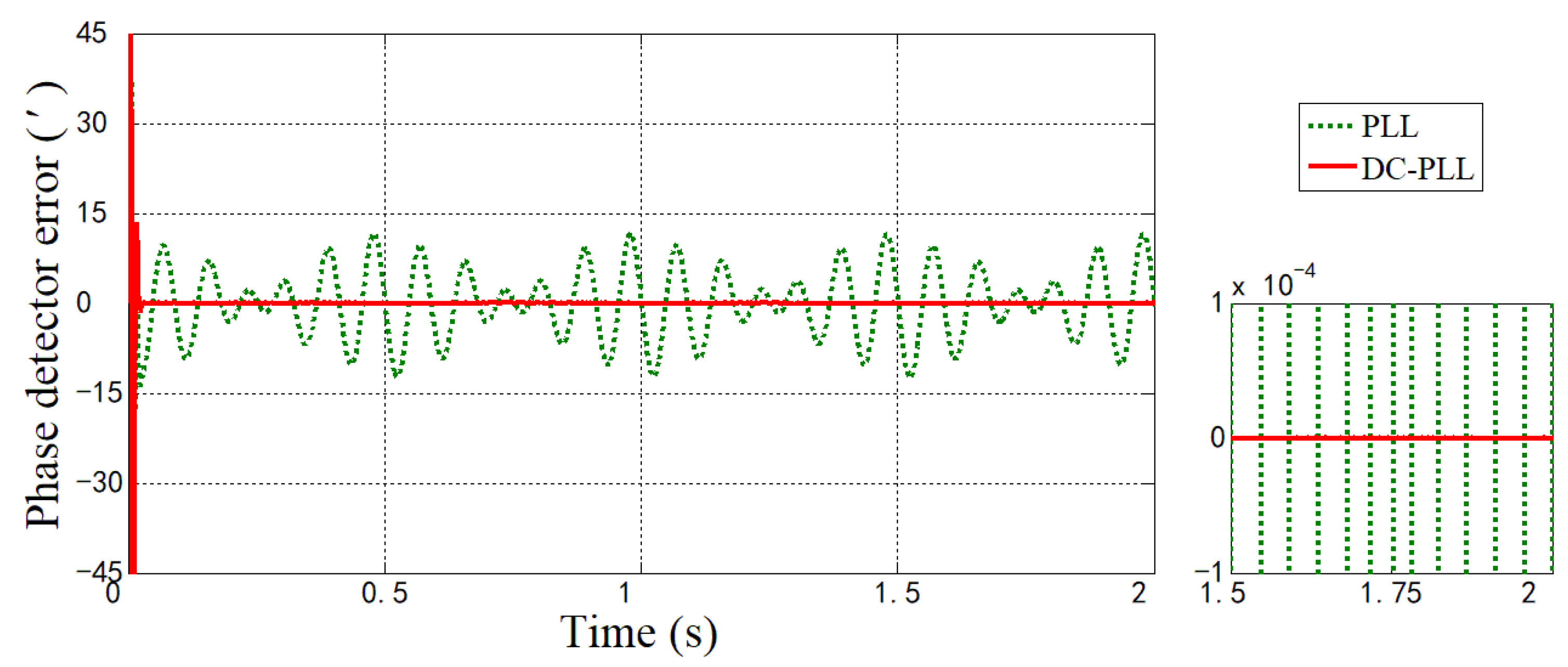
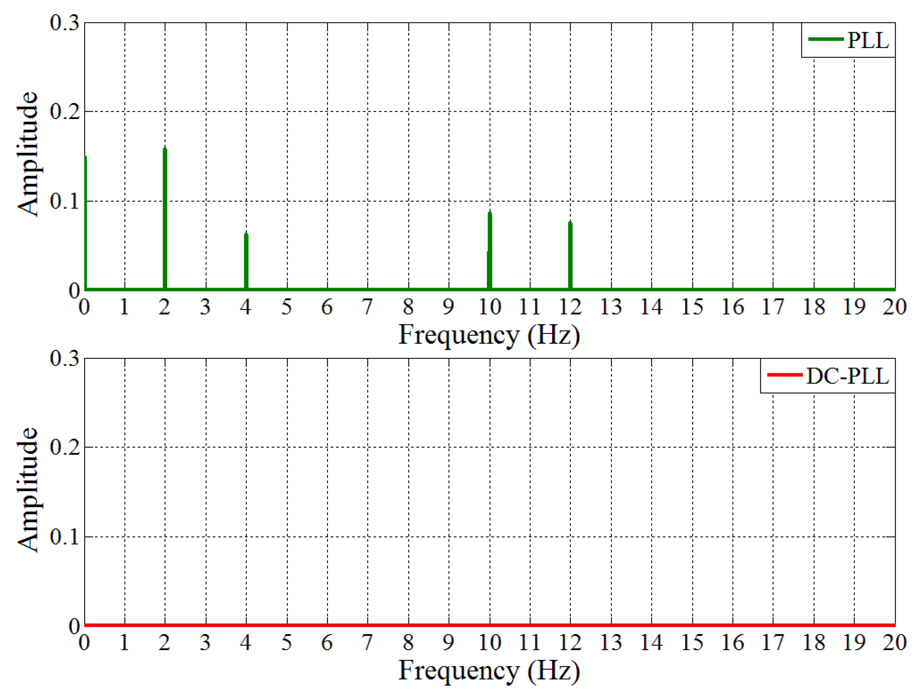
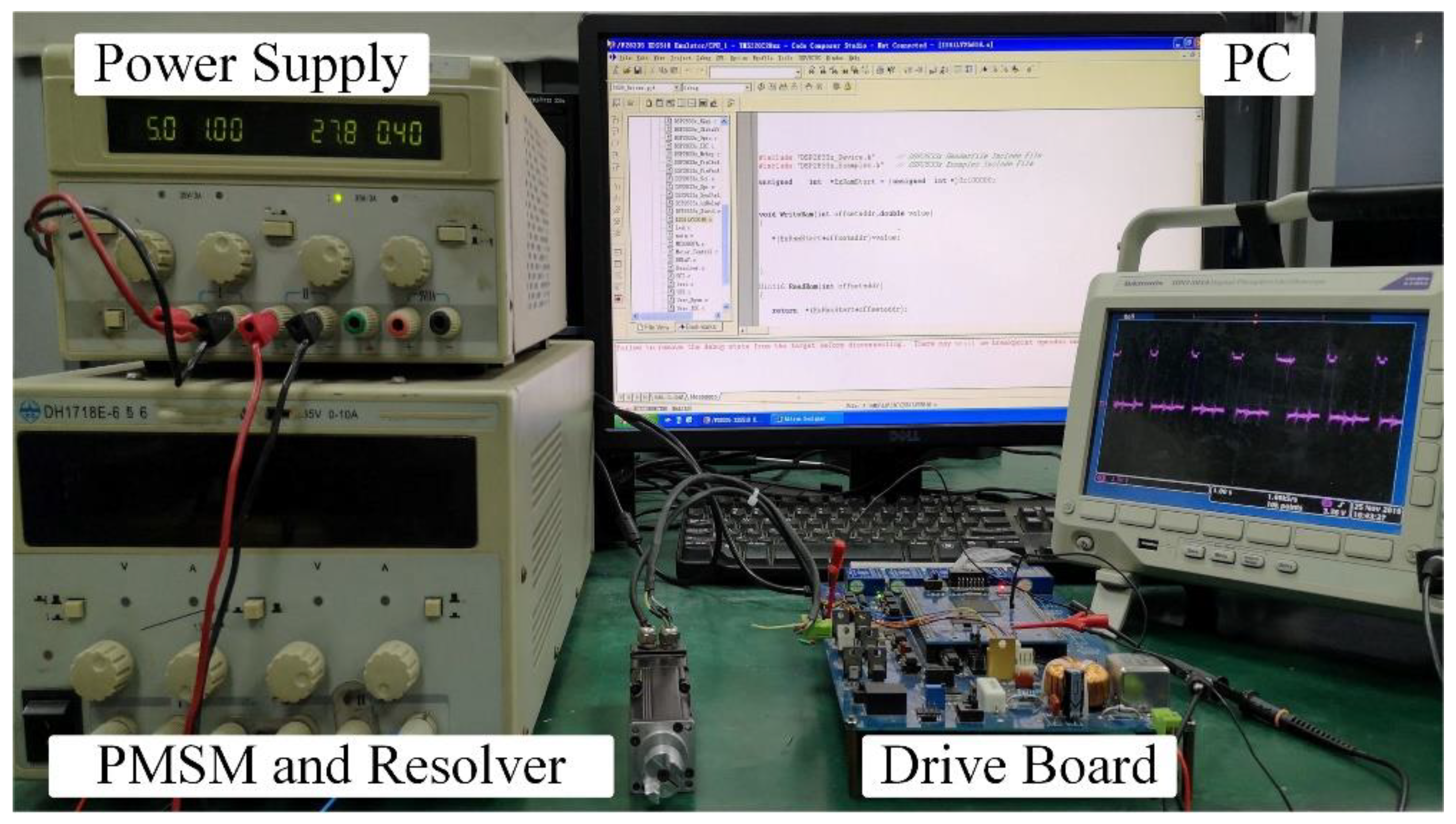
4.2. Experiment Results
5. Conclusions
Author Contributions
Funding
Institutional Review Board Statement
Informed Consent Statement
Data Availability Statement
Conflicts of Interest
References
- Sabatini, V.; Benedetto, M.D.; Lidozzi, A. Synchronous adaptive resolver-to-digital converter for FPGA-based high-performance control loops. IEEE Trans. Instrum. Meas. 2019, 68, 3972–3982. [Google Scholar] [CrossRef]
- Yepes, A.G.; Lopez, O.; Gonzalez-Prieto, I.; Duran, M.J.; Doval-Gandoy, J. A Comprehensive survey on fault tolerance in multiphase AC drives, part 1: General overview considering multiple fault types. Machines 2022, 10, 208. [Google Scholar] [CrossRef]
- Saneie, H.; Nasiri-Gheidari, Z.; Tootoonchian, F. Structural design and analysis of a high reliability multi-turn wound-rotor resolver for electric vehicle. IEEE Trans. Veh. Technol. 2020, 69, 4992–4999. [Google Scholar] [CrossRef]
- Estrabis, T.; Gentil, G.; Rordero, R. Development of a resolver-to-digital converter based on second-order difference generalized predictive control. Energies 2012, 14, 459. [Google Scholar] [CrossRef]
- Khaburi, D.A. Software-based resolver-to-digital converter for DSP-based drives using an improved angle-tracking observer. IEEE Trans. Instrum. Meas. 2012, 61, 922–929. [Google Scholar] [CrossRef]
- Hanselman, D.C. Resolver signal requirements for high accuracy resolver-to-digital conversion. IEEE Trans. Ind. Electron. 1990, 37, 556–561. [Google Scholar] [CrossRef]
- Kaul, S.K.; Tickoo, A.K.; Koul, R.; Kumar, N. Improving the accuracy of low-cost resolver-based encoders using harmonic analysis. Nucl. Instrum. Methods Phys. Res. A 2008, 586, 345–355. [Google Scholar] [CrossRef]
- Hanselman, D.C. Techniques for improving resolver-to-digital conversion accuracy. IEEE Trans. Ind. Electron. 1991, 38, 501–504. [Google Scholar] [CrossRef]
- Robinson, R.B. Inductance coefficients of rotating machines expressed in terms of winding space harmonic. Proc. Inst. Electr. Eng. 1964, 111, 769–774. [Google Scholar] [CrossRef]
- Ge, X.; Zhu, Z.Q. A novel design of rotor contour for variable reluctance resolver by injecting auxiliary air-gap permeance harmonics. IEEE Trans. Energy Convers. 2016, 31, 345–353. [Google Scholar] [CrossRef]
- Wang, F.; Shi, T.; Yan, Y.; Wang, Z.; Xia, C. Resolver-to-digital conversion based on acceleration-compensated angle tracking observer. IEEE Trans. Instrum. Meas. 2019, 68, 3494–3502. [Google Scholar] [CrossRef]
- Bahari, M.; Davoodi, A.; Saneie, H.; Tootoonchian, F.; Nasiri-Gheidari, Z. A new variable reluctance PM-resolver. IEEE Sens. J. 2020, 20, 135–142. [Google Scholar] [CrossRef]
- Sarma, S.; Agrawal, V.K.; Udupa, S. Software-based resolver-to-digital conversion using a DSP. IEEE Trans. Ind. Electron. 2008, 55, 371–379. [Google Scholar] [CrossRef]
- Hou, C.; Chiang, Y.; Lo, C. DSP-based resolver-to-digital conversion system designed in time domain. IET Power Electron. 2014, 7, 2227–2232. [Google Scholar] [CrossRef]
- Kamf, T.; Abrahamsson, J. Self-sensing electromagnets for robotic tooling systems: Combining sensor and actuator. Machines 2016, 4, 16. [Google Scholar] [CrossRef]
- Wang, S.; Kang, J.; Degano, M.; Buticchi, G. A Resolver-to-digital conversion method based on third-order rational fraction polynomial approximation for PMSM control. IEEE Trans. Ind. Electron. 2019, 66, 6383–6392. [Google Scholar] [CrossRef]
- Herrejón-Pintor, G.A.; Melgoza-Vázquez, E.; Chávez, J.D.J. A modified SOGI-PLL with adjustable refiltering for improved stability and reduced response time. Energies 2022, 15, 4253. [Google Scholar] [CrossRef]
- Linares-Flores, J.; García-Rodríguez, C.; Sira-Ramírez, H.; Ramírez-Cárdenas, O.D. Robust backstepping tracking controller for low-speed PMSM positioning system: Design, analysis, and implementation. IEEE Trans. Ind. Inform. 2015, 11, 1130–1141. [Google Scholar] [CrossRef]
- Bergas-Jané, J.; Ferrater-Simón, C.; Gross, G.; Ramírez-Pisco, R.; Galceran-Arellano, S.; Rull-Duran, J. High-accuracy all-digital resolver-to-digital conversion. IEEE Trans. Ind. Electron. 2012, 59, 326–333. [Google Scholar] [CrossRef]
- Zhang, J.; Wu, Z. Composite state observer for resolver-to-digital conversion. Meas. Sci. Technol. 2017, 28, 065103. [Google Scholar] [CrossRef]
- Sivappagari, C.M.R.; Konduru, N.R. High accuracy resolver to digital converter based on modified angle tracking observer method. Sens. Transducers 2012, 144, 101–112. [Google Scholar]
- Zhang, J.; Wu, Z. Automatic calibration of resolver signals via state observers. Meas. Sci. Technol. 2014, 25, 2223–2237. [Google Scholar] [CrossRef]
- Wu, Z.; Li, Y. High-accuracy automatic calibration of resolver signals via two-step gradient estimators. IEEE Sens. J. 2018, 18, 2883–2891. [Google Scholar] [CrossRef]
- Shi, T.; Hao, Y.; Jiang, G.; Wang, Z.; Xia, C. A method of resolver-to-digital conversion based on square wave excitation. IEEE Trans. Ind. Electron. 2018, 65, 7211–7219. [Google Scholar] [CrossRef]
- Farid, T. Effect of damper winding on accuracy of wound-rotor resolver under static-, dynamic-, and mixed-eccentricities. IET Power Electron. 2018, 12, 845–851. [Google Scholar]
- Saneie, H.; Alipour-Sarabi, R.; Nasiri-Gheidari, Z.; Tootoonchian, F. Challenges of finite element analysis of resolvers. IEEE Trans. Energy Convers. 2019, 34, 973–983. [Google Scholar] [CrossRef]
- Pecly, L.; Schindeler, R.; Cleveland, D.; Hashtrudi-Zaad, K. High-precision resolver-to-velocity converter. IEEE Trans. Instrum. Meas. 2017, 66, 2917–2928. [Google Scholar] [CrossRef]
- Ge, X.; Zhu, Z.Q.; Ren, R.; Chen, J.T. Analysis of windings in variable reluctance resolver. IEEE Trans. Magn. 2015, 51, 8104810. [Google Scholar] [CrossRef]


| Cases | Case 1 | Case 2 | Case 3 | |
|---|---|---|---|---|
| PLL | AVG | 9.008 | 9.104 | 9.747 |
| STD | 8.747 | 9.012 | 8.391 | |
| Compensate β | AVG | 2.009 × 10⁻⁵ | 0.071 | 0.176 |
| STD | 5.996 | 6.392 | 5.847 | |
| DC-PLL | AVG | 3.811 × 10⁻¹² | 0.036 | 4.260 × 10⁻⁵ |
| STD | 4.721 × 10⁻¹¹ | 7.468 × 10⁻⁴ | 0.1599 | |
| Cases | Case 1 | Case 2 | Case 3 | |
|---|---|---|---|---|
| PLL | AVG | 2.211 × 10⁻⁷ | 0.412 | 7.278 × 10⁻¹² |
| STD | 5.819 | 17.814 | 6.443 | |
| Compensate β | AVG | 2.195 × 10⁻⁷ | 0.390 | 5.939 × 10⁻¹² |
| STD | 5.664 | 17.350 | 6.323 | |
| DC-PLL | AVG | 2.586 × 10⁻¹⁰ | 0.379 | 1.288 × 10⁻¹² |
| STD | 5.387×10⁻¹⁰ | 0.002 | 1.733 | |
| PMSM | Resolver | ||
|---|---|---|---|
| Pole pairs | 2 | Pole pairs | 1 |
| Rated speed | 3000 r/min | Excitation frequency | 10 kHz |
| Torque constant | 0.15 Nm/A | Electrical error | 10′ |
| Phase resistance | 8 Ω | Input impedance | 95 ± 14 Ω |
| Phase inductance | 10 mH | Quadrature error | 0.3° |
| Cases | |||
|---|---|---|---|
| PLL | AVG | 2.482 × 10⁻⁴ | 359.999504 |
| STD | 37.335 | 32.6144 | |
| DC-PLL | AVG | 3.620 × 10⁻⁵ | 359.999721 |
| STD | 10.443 | 8.333 | |
Publisher’s Note: MDPI stays neutral with regard to jurisdictional claims in published maps and institutional affiliations. |
© 2022 by the authors. Licensee MDPI, Basel, Switzerland. This article is an open access article distributed under the terms and conditions of the Creative Commons Attribution (CC BY) license (https://creativecommons.org/licenses/by/4.0/).
Share and Cite
Wang, R.; Wu, Z. Suppressing Quadrature Error and Harmonics in Resolver Signals via Disturbance-Compensated PLL. Machines 2022, 10, 709. https://doi.org/10.3390/machines10080709
Wang R, Wu Z. Suppressing Quadrature Error and Harmonics in Resolver Signals via Disturbance-Compensated PLL. Machines. 2022; 10(8):709. https://doi.org/10.3390/machines10080709
Chicago/Turabian StyleWang, Rui, and Zhong Wu. 2022. "Suppressing Quadrature Error and Harmonics in Resolver Signals via Disturbance-Compensated PLL" Machines 10, no. 8: 709. https://doi.org/10.3390/machines10080709