Article

Estimations of Compressor Stall and Surge Using Passage Stall Behaviors

School of Mechanical Engineering, Iran University of Science and Technology, Tehran 16846-13114, Iran
*
Author to whom correspondence should be addressed.
Machines 2022, 10(8), 706; https://doi.org/10.3390/machines10080706
Submission received: 30 May 2022 / Revised: 17 June 2022 / Accepted: 22 June 2022 / Published: 18 August 2022
(This article belongs to the Section Turbomachinery)

Abstract

:
The predictions of the onset of rotating stall and surge are very important in the preliminary design stage of a compressor. Rotating stall and surge are complex instabilities that cause efficiency loss and reduced pressure rise, and, therefore, compressor designers attempt to avoid them in the design stage. There are many criteria for predicting stability limits, including empirical, theoretical, and numerical investigations in the literature. However, these investigations have important limitations. The present study establishes a new method in which the stall and post-stall behavior of a compressor is estimated by an equivalent reconstructed compressor using special combinations of single-passage flow behavior in different mass flow rates. The combinations are generated such that pre-stall, in-stall, and surge flow regimes and between one and eight stall cells are reproduced in the full-annulus compressor. The method requires the least computational requirements and is time efficient. The results indicate that secondary flow total energy and spectral entropy are indeed correlated with compressor operating conditions. The predictions of the onset of stall and surge for the investigated compressor show good agreement with the experimental data.

1. Introduction

Rotating stall and surge are aerodynamic instabilities that limit the performance of a compressor under high loading conditions. Rotating stall induces large vibrations of blades that affects blade life span, pressure ratio, and isentropic efficiency degradation [1]. Surge, on the other hand, is a more detrimental instability that affects the whole engine and involves overall flow breakdown [2]. Consequently, there is a great tendency to detect and delay the onset of instabilities in the preliminary design stage. While the operating points that instabilities initiate are easily detected in experimental works by accompanying noise and mechanical vibration with a minimal error, it was reported by Dixon [3] that the detection of stall inception in numerical investigations is a difficult task. A difficulty associated with numerical detection of the instabilities is the necessity of time-accurate simulations of rotating stall and surge phenomena due to their unsteady nature. Another difficulty is that no assumption regarding spatial periodicity of instabilities can be made. Preliminary attempts to model and predict stall and post-stall behavior are composed of estimating blade stall and perturbation analysis [4,5]. It should be noted that blade stall in these studies refers to maximum pressure rise that a blade row can sustain without incurring stall. In this regard, the diffusion factor and de Haller and Koch’s stalling pressure rise coefficient have been developed [6]. In addition to these early stall correlations, some other studies have attempted to model and predict the stability limits theoretically or numerically. One of the famous theoretical investigations was developed by Greitzer [7,8]. According to his investigation, there is a critical B parameter in which under it, a compressor experiences rotating stall, and above it, it will surge. Apart from these early studies that are focused on finding criteria for the onset of stall and surge, there are other studies on modeling the properties of rotating stall cells and their propagation speed [9,10,11,12].
Gogoi [13] employed a CFD-based model to capture the onset of rotating stall and surge. The model employs quasi-3D Euler equations, and the results indicate that the two modes of instabilities were captured reasonably well for two compressors. However, the comparison of the numerical frequencies to the corresponding experimental results indicates that there is some discrepancy. A limitation of the model is that the flow is one-dimensional in inlet guide vanes, rotor, stator, and exit guide vanes. Furthermore, the model is limited to a single compressor without any extra component unless further governing equations are added. Benavides [14] employed a new stability theorem based on the ratio of axial solidity of the rotor to a function that measures the potential for escaping particles. The model is based on a reformulated stability theorem that is physically and mathematically valid in all the operating points. The reformulation resolves the limitation of the original stability theorem in which several asymptotic behaviors in some operating points were encountered. This model is capable of detecting stall inception for both rotors and stators and possible reverse flow regimes and captures the full compressor map. The assumptions of the model are steady and homogeneous fluid properties at the inlet and outlet. However, once the operating point is beyond stall, these assumptions break down, and the stability theorem cannot be utilized. The main drawback concerning the results of this study is that the prediction of the onset of surge is not specified, and the stability theorem is formulated for a single compressor without any extra component unless extra governing equations are added. An improvement to the previous model was reported by Benavides [15]. The improved model extends the application of the stability theorem up to the surge operating points as well as the stall inception. In this regard, the effects of rotor efficiency, outlet deviation angle, and inlet incidence angle have been investigated. Although the improved model can capture the behavior of the compressor up to surge, it suffers the same limitation as the previous models in which the model cannot be applied to a compressor with an extra component. In other investigations, the analysis of time traces of pressure and velocity signals and flow-field changes have been employed to predict stall and post-stall behavior. It was proposed by Vo [16] that the spillage of tip clearance flow to adjacent blades and tip clearance backflow are indicators of spike-type stall inception. A set of continuous mass flow rate reduction [17], breakdown of signal periodicity [18], continuous reduction of pressure ratio, mass flow and efficiency [19], sudden drop in pressure rise coefficient [20], absence of blade passing frequency and its harmonics [21], as well as the influence of geometry, mesh, turbulence model, steady and transient simulations [22] on the detection of stall points, were investigated numerically.
The above investigations have been very useful in predicting stall inception up to surge condition. However, these studies have important limitations: First, the empirical approach is limited to the estimation of blade stall and is a very approximation of a compressor’s overall instabilities. Second, most of the theoretical investigations have been developed for a specific compressor without any further components. As a consequence, their validity for all compressors is questionable, and unless extra equations are added, these models cannot be applied to a compressor with an extra component such as the one in this study with a casing treatment. Third, most numerical approaches employ a correlation between compressor operating conditions and performance parameters to predict the stability limits. However, since performance reduction is not significant for the compressor utilized in this study and numerical error, these correlations are not useful, which will further complicate the estimation of stability limits, and a transient simulation including all the passages (full annulus) is required.
The present study employs a new approximation method in which the onset of stall and surge of a compressor is estimated by reconstructing a full-annulus compressor by utilizing the special combinations of single-passage simulations at different mass flow rates. The main advantage of the approximation method is that it requires the least computational requirements and is quick. Total energy due to secondary flow oscillations and spectral entropy will be used as criteria to detect the onset of instabilities in an axial-flow compressor. In addition, an estimation of stall cell frequency for between one and eight stall cells will be provided.

2. Stall Inception Theory

In order to explain the proposed model of prediction of stall inception and surge in this paper, the whole stalling process of a low-speed compressor is discussed in this section. The model has been developed based on the basic stalling process of previous experimental and analytical research [1,2,3,6,7,8,23], in which the whole operating conditions from pre-stall to stall and in-stall conditions are considered. The basic process of stalling a compressor is composed of several conditions: As a compressor is operating between the maximum mass flow to the design operating points, the compressor provides a pressure rise, and no disturbances exist in the blade row. As the mass flow is reduced, small disturbances in the form of flow separation appear at the blade suction side. These separations form due to adverse pressure gradient and boundary layer effects. With the subsequent reduction in mass flow, the small disturbances grow in size and accumulate in the blade passages. While the compressor is still operating in pre-stall condition, the disturbances grow in size and cover several blade passages. Up to now, the disturbances are confined to the blade passages and are not moving along the blade row. Once the mass flow reaches a critical value, instead of all blades stalling together as is expected, all the blades do not stall simultaneously. At some point, the stall cell, which is made up of low momentum regions, starts to propagate along the blade row. Afterward, the disturbances merge together and form a number of stall cells with a further reduction in mass flow. Eventually, the stall cells merge together and form a big stall cell. The propagation speed of the stall cells is approximately 20–80% of the rotor speed [24]. The number of stall cells that forms in the annulus is dependent on compressor design and flow behavior and cannot be predicted accurately for a newly designed compressor [1]. With further reduction in the mass flow, the compressor encounters the global surge condition and, subsequently, breakdown of the compressor may occur. It has been stated that rotating stall usually precedes surge. An example of a stall cell formation and propagation is shown in Figure 1.

3. Developed Model

Based on the stages of stall inception discussed in the previous section, the stall inception process of a compressor can be categorized according to its disturbances into no disturbance, formation, and growth of the disturbances. Although the final number of stall cells that forms in the annulus is not known in advance, the first appearance of a stall cell is confined to one stall cell that may grow into a number of stall cells with a further reduction in mass flow. Afterward, the disturbances reach a critical size and start to move along the blade row. Since the number of stall cells is not known beforehand, a number of stall cells should be assumed. Here, between 1 and 8 stall cells are considered for demonstration. The proposed model is composed of four steps.

3.1. Single-Passage Computations

A series of unsteady single-passage simulations is conducted to cover the whole operating range of a compressor from maximum mass flow to stall and in-stall operating conditions. These single-passage simulations are taken as a basis for reconstructing the full-annulus compressor. Here, experimental compressor data were employed for demonstration and validation of the developed model. The simulated mass flow rates are given in Table 1, while ‘A’ refers to the biggest mass flow and ‘K’ refers to the lowest mass flow and corresponds to the in-stall condition. The details of the experimental compressor and the numerical details are given in the next sections. A numerical probe is placed near the casing and adjacent to the rotor leading edge and records the variation in static pressure with time for every mass flow during the numerical simulations. The recorded static pressure by the numerical probe will be used to generate a pressure signal, which is the variation in static pressure versus time for every mass flow. The pressure signals will be used for further processing to detect the compressor operating conditions and frequency analysis in the next sections.

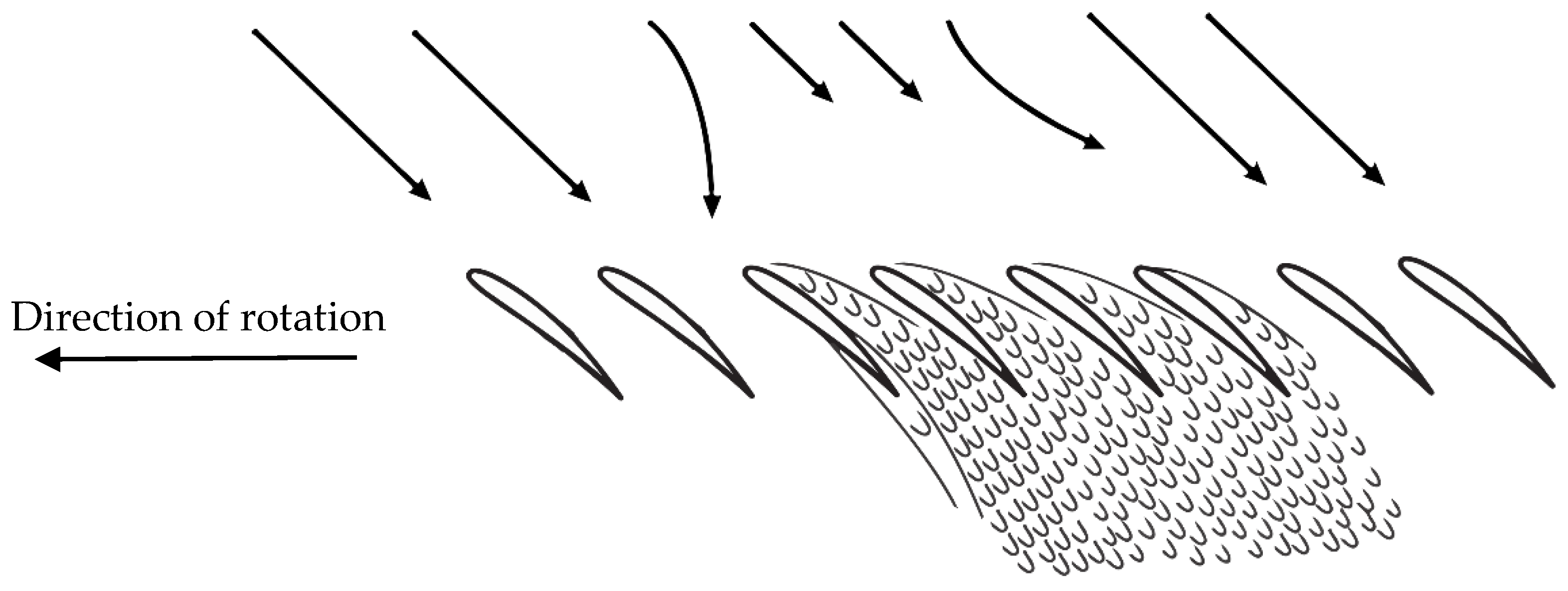
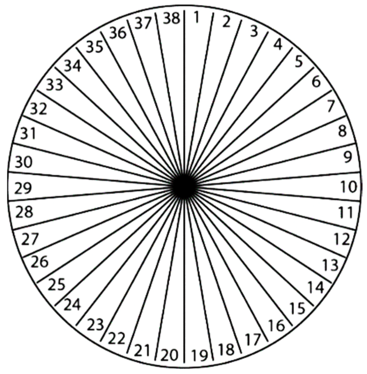
3.2. Reconstruction of Full-Annulus Compressor Conceptually

The full-annulus compressor is reconstructed conceptually based on the special combinations of the single-passage simulations from Table 1 to cover the whole operating range of the compressor, including pre-stall, stall, and in-stall operating conditions. Here, a number of 38 rotor passages is utilized since the experimental compressor has 38 rotor blades, as shown schematically in Figure 2.
In order to reflect the stalling process of a compressor containing one stall cell at its final stage, the whole process in which no disturbance exists initially and small disturbances form and grow in size and reach a critical size are considered. These operating conditions are reflected in each row in Table 2, respectively. The full-annulus mass flow for every row is calculated as the summations of all the mass flows distributed in the 38 passages. In the first row, the condition in which no disturbance exists in all 38 passages is considered. As a result, the biggest mass flow, “A,” is distributed among all the blade passages. Since it was assumed that one stall cell is formed at its final stage for this case, two slightly lower mass flows, “B,” are distributed in the middle of the second row, while the remaining mass flow rates are kept constant. In order to reflect the operating conditions from the maximum mass flow to the design operating points, the two mass flow rates in the previous row, in addition to their adjacent ones, are lowered one step further according to Table 1. Afterward, the mass flow rates are lowered continuously and gradually with the same patterns to reflect the later operating conditions, including the growth of the disturbances. The final row contains the lowest mass flow, “K,” in every 38-blade passage.
The reconstruction of two stall cells at its final stage differs from one stall cell in that two groups of two mass flow rates are selected as a basis at the second row in Table 3. These mass flow and their adjacent ones are lowered gradually with the same patterns to form two stall cells. The reconstructions of three to eight stall cells are performed likewise; however, three groups of two mass flow rates are selected as a basis at the second row and so on, as shown in Table 4, Table 5, Table 6, Table 7, Table 8 and Table 9. Once the reconstructions of the full-annulus compressor are complete for all the number of stall cells, a pressure signal is generated for every total mass flow and stall cell number in the next section.

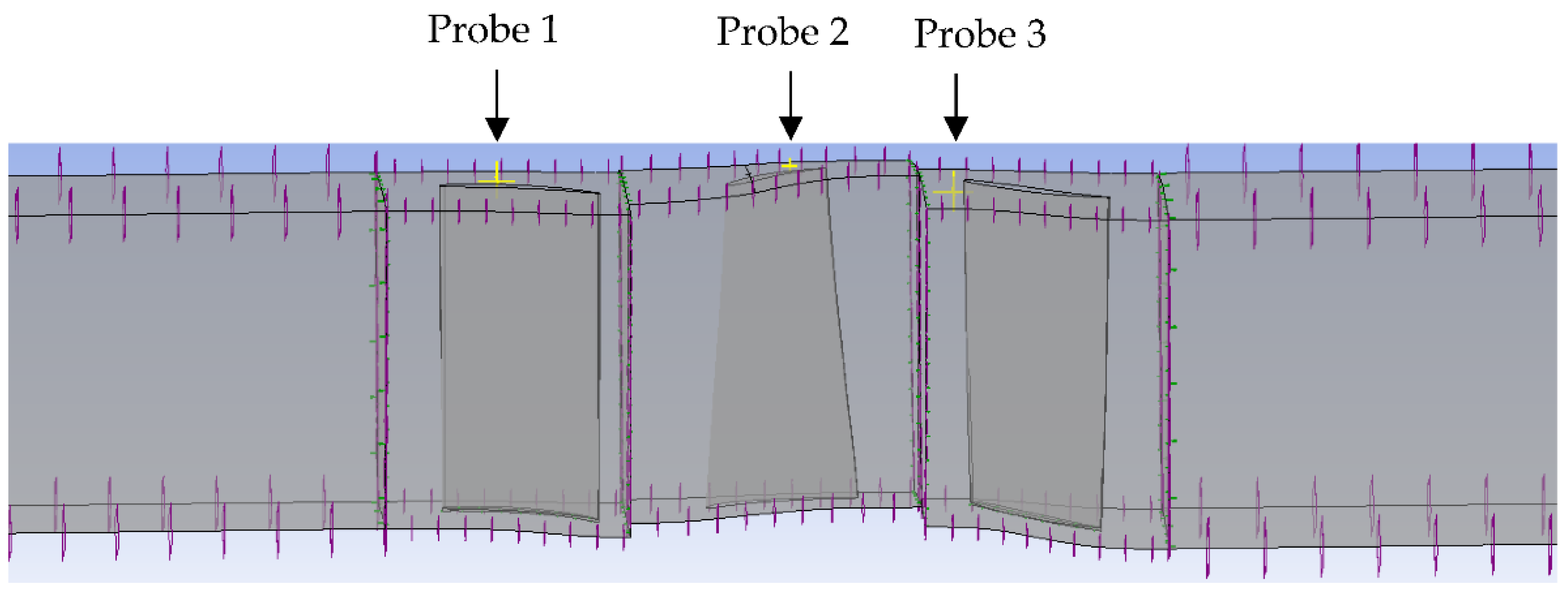
3.3. Generation of Pressure Signals

After the reconstructions of all the number of the stall cells are ready conceptually, a pressure signal is generated for every total mass flow and stall cell number. The pressure signal for every total mass flow is generated by placing the recorded static pressures in Section 3.1 consecutively. A fixed number of 2000 static pressure should be used to prevent numerical error. For example, in order to generate a pressure signal for the configuration consisting of the biggest mass flow, “A,” among the 38 passages, the 2000 static pressure is repeated 38 times successively. Consequently, a signal containing 76,000 static pressure is generated for every total mass flow. The total numbers of pressure signals are comprised of 29, 20, 17, 15, 14, 13, 14, and 15 for one to eight stall cells, respectively. This equals 137 pressure signals for all the number of stall cells and mass flow rates. The signals represent the behavior of the full-annulus compressor and are used in calculations of total energy, spectral entropy, and stall cell frequency in the next sections.

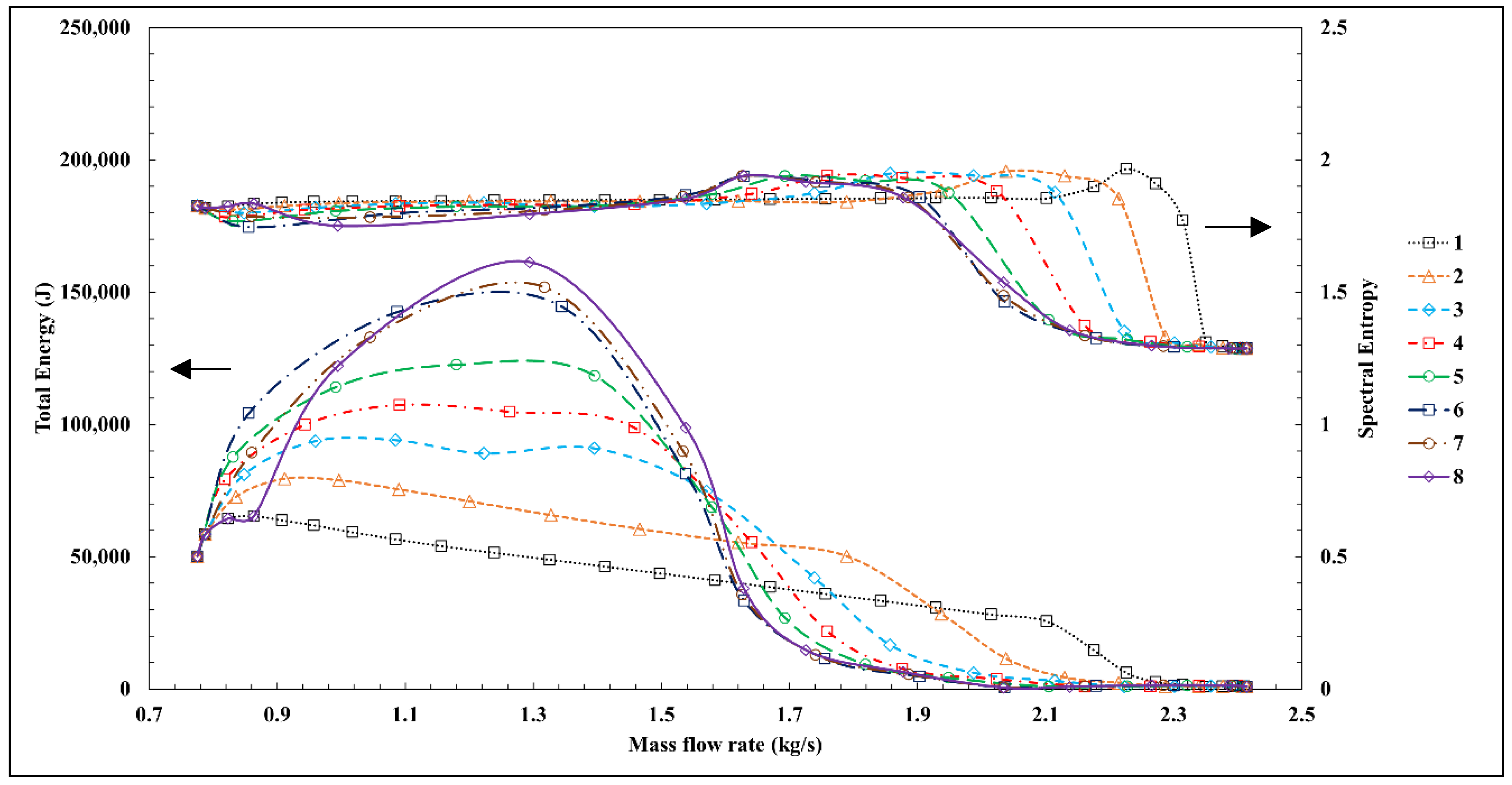
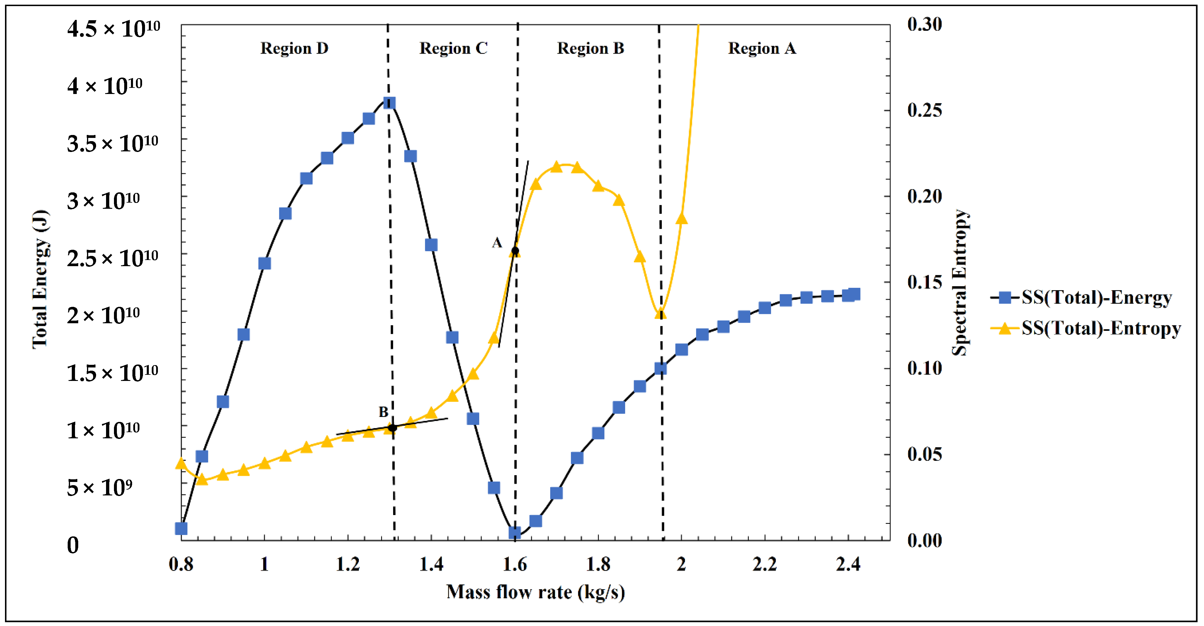
3.4. Calculations of Total Energy and Spectral Entropy

Once the pressure signals are set up for every total mass flow and the number of stall cell, the total energy and the spectral entropy are calculated. The total energy in the context of this study represents the total energy originating from secondary flow oscillations.
The total energy (E) of a signal is mathematically defined as:
E = f t 2 d t
where f is the pressure signal containing 76,000 static pressures computed in previous section.
The spectral entropy (SE) is mathematically defined as:
S E = i = 1 N p i log 10 p i
where the probability distribution ( p i ) is defined as normalized power distribution in the frequency domain:
p i = X i j = 1 N X j
Spectral entropy is a generalization form of Shannon’s information theory and represents the expected (average) uncertainty in a signal. In general, lower spectral entropy corresponds to a higher probability, while higher spectral entropy corresponds to a lower probability. Zero entropy represents a special case in which the outcome of an event is known with certainty. Figure 3 shows the effects of between 1 and 8 stall cells on the total energy and the spectral entropy based on the stalling patterns defined in Table 2, Table 3, Table 4, Table 5, Table 6, Table 7, Table 8 and Table 9.
As can be seen from Figure 3, at higher mass flow rates than 2.35 kg/s, the total energy for all the number of stall cells is at its lowest amount. This signifies that the vibration and noise of the compressor are minimal. Furthermore, all the stall cell numbers have identical spectral entropy, which shows that the probability of stall cell formation is similar.
With the reduction in the mass flow to 2.35 kg/s, the total energy for all the stall cells maintains its lowest amount and the spectral entropy of the one stall cell case begins to rise. This shows that the likelihood of stall cell formation for this case will decrease. Since all the numbers of stall cells still have an equal probability of formation and the total energy for all the stall cells is still at its lowest amount, this operating point is considered pre-stall.
With a further reduction in the mass flow to 2.3 kg/s, the total energy of the one stall cell case and the spectral entropy of the two stall cells case begin to increase. The increase in the total energy signifies that vibration and noise rise. Moreover, the increase in the spectral entropy shows that the probability of stall cell formation for this case will reduce. Again, this operating point is considered pre-stall.
At about 2.1 kg/s, the total energy for the rest of the stall cells begins to increase. This could be interpreted as that there is a probability that the compressor is approaching stall condition. Since rotating stall usually precedes surge, this operating point is considered approaching stall and away from surge.
When considering the mass flow rates between 1.5 kg/s to 2.1 kg/s, the distributions of the spectral entropy change slightly. As the mass flow rate approaches 1.5 kg/s, the spectral entropy for all the number of stall cells suddenly converges to a point. This sudden convergence can be interpreted as the compressor undergoing a significant change in its flow behavior. Furthermore, increased total energy indicates that vibration and noise are intensified. The identical probability of formation, change of flow behavior, and increased total energy signify that the surge condition is imminent.
As the mass flow rate is reduced further than 1.5 kg/s, the total energy still rises and subsequently decreases. The sudden reduction in total energy can be explained as the mass flow rate decreases, and the axial velocity component decreases too, which, in turn, reduces the kinetic energy of secondary flow oscillations. Moreover, the convergence of the spectral entropy to a point at 1.5 kg/s changes, and different spectral entropy appears.
It can be concluded from the analysis of this section that at higher mass flow rates than 2.35 kg/s, a unique solution exists because it is away from the instabilities. As the mass flow rate is reduced and stall is approached, no unique solution exists anymore, and the solution bifurcates. This is due to the unstable operation of the compressor while approaching instabilities, in which a marginal change of the throttling valve can transform the operating point from pre-stall to in-stall condition. To further define the conditions that the compressor experiences rotating stall and surge conditions, statistical ANOVA analysis is performed in the next section.

3.5. ANOVA Analysis

One-way ANOVA analysis is performed in this section to validate the results of the total energy and the spectral entropy from a statistical point of view. Table 10 and Table 11 present the ANOVA analysis for the total energy and the spectral entropy. As the values of the F-tests are large and the probability that F takes larger values than the F-tests is zero for both of the cases, it is concluded that the null hypothesis is false for the total energy and the spectral entropy. The null hypothesis assumes that any observed significance is entirely random.

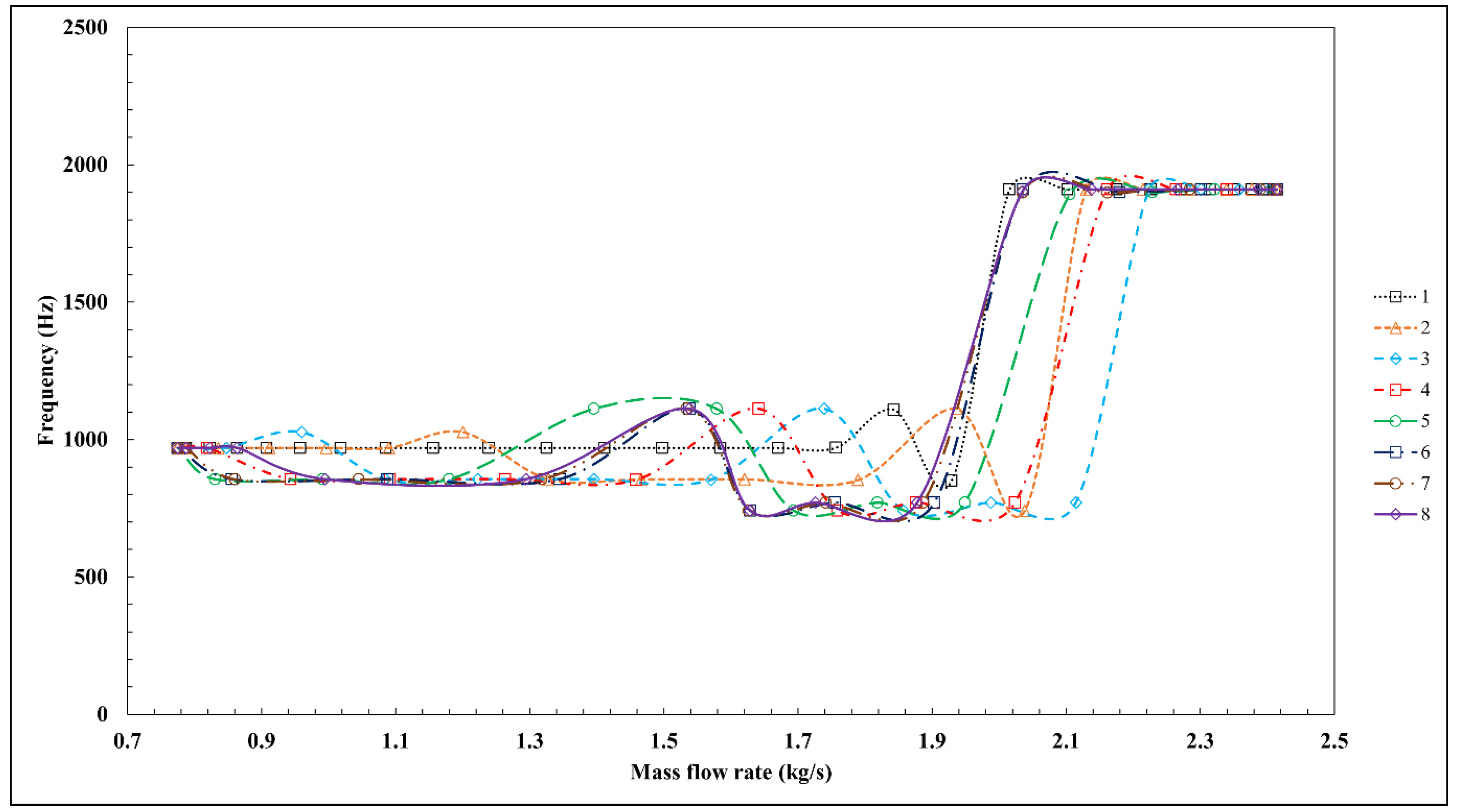
3.6. Stall Cell Frequency

In the preceding section, the pressure signals consisting of the variation in static pressure versus time were generated for every total mass flow and stall cell number. The pressure signals are used in this section to estimate the frequencies in the full-annulus compressor. Figure 4 shows the influence of the number of stall cells on the frequency from the maximum mass flow to stall and in-stall conditions. The frequency in this figure has been obtained by performing an FFT analysis of the corresponding stall cell number and mass flow and represents the peak frequency in the full-annulus configuration for every total mass flow. The total number of performing FFT analyses is equal to 137 times. The frequency in the context of this paper corresponds to the frequency of formation and propagation of the stall cells based on the full-annulus compressor approximation. As can be seen from Figure 4, at higher mass flow rates, the blade passing frequency (BPF) at 1900 Hz exists for all the number of stall cells since no disturbance has been formed in the annulus yet. As the mass flow is reduced, secondary flow oscillations form and new frequencies related to these disturbances appear. Although the distributions of the frequencies vary slightly with the reduction in mass flow, the change in the frequencies is limited to a specific band between 700 Hz and 1100 Hz. The final frequency for all the number of stall cells is 969.6 Hz when the stall cells reach a fully developed condition. The analysis in this section investigates the possibility of defining criteria to detect compressor operating conditions based on the variation in frequencies as the mass flow is reduced. The figure shows that new frequencies develop at lower mass flow rates below 2.1 kg/s, but the distributions of the frequencies do not vary significantly toward the lower mass flow rates. In particular, no significant change of frequencies occurs at 1.6 kg/s, where surge instability is estimated to commence. Consequently, it can be concluded that a criterion based on the frequency change can show a rough estimation of the onset of rotating stall, but it cannot be used to estimate the onset of the global instability or surge condition.

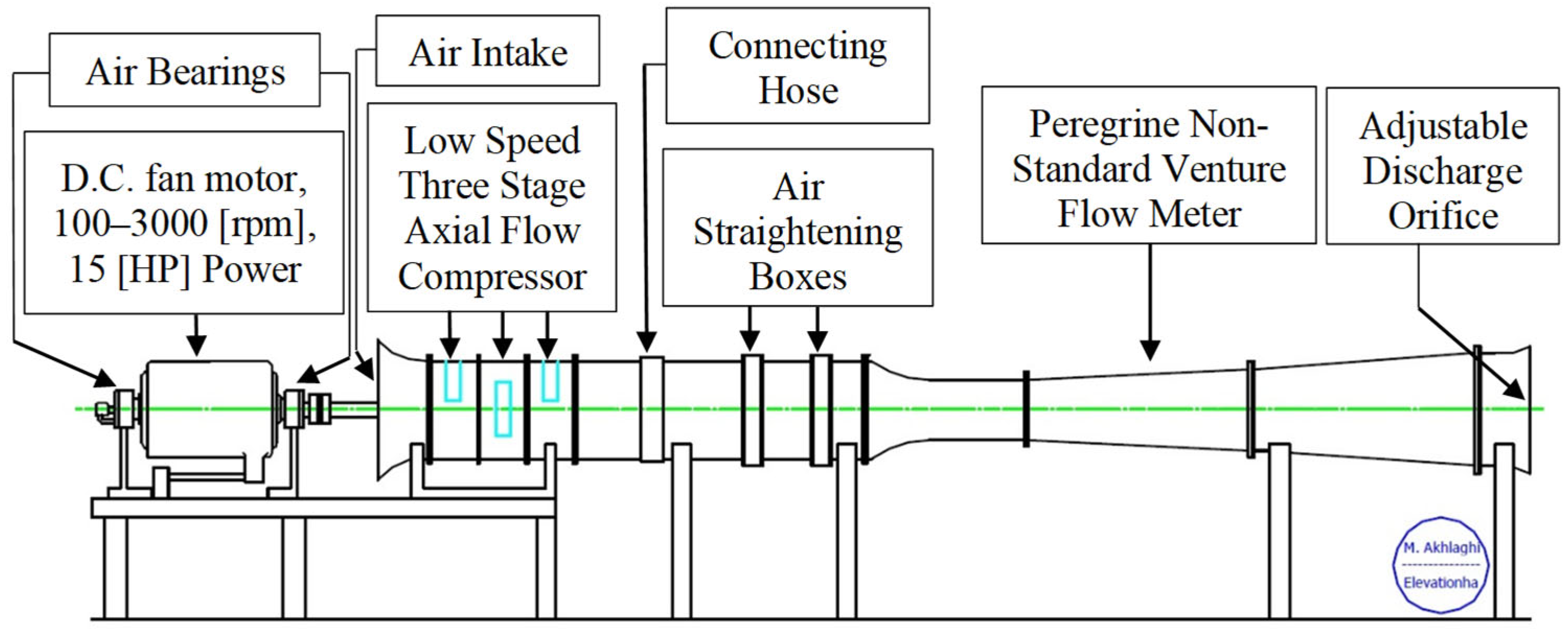
4. Experimental Compressor

This research utilizes experimental compressor data to demonstrate and validate the application of the approximation method. The configuration under investigation is the axial compressor with the casing treatment employing 23.2% exposure. This research compressor was named Peregrine and was tested at Cranfield University in 2001 [25,26]. The test rig consisted of an electric motor, three repeating stages compressor, a bellmouth inlet, and an outlet ducting. The rotor shaft was driven by an electric motor at a design speed of 3000 rpm. A schematic of the research test rig is shown in Figure 5.
A brief specification of the compressor is summarized in Table 12. The blades feature a free vortex design.

5. Numerical Details

5.1. Governing Equations

The governing equations that are solved consist of continuity, momentum, and turbulence transport equations. The flow is assumed to be incompressible since the compressor is operating at a low speed.

5.2. Turbulence Model

The turbulence was modeled by the shear stress transport k ω . The SST turbulence model benefits from accurate representations of k ω near-wall regions and freestream independence of k ε model away from wall regions.

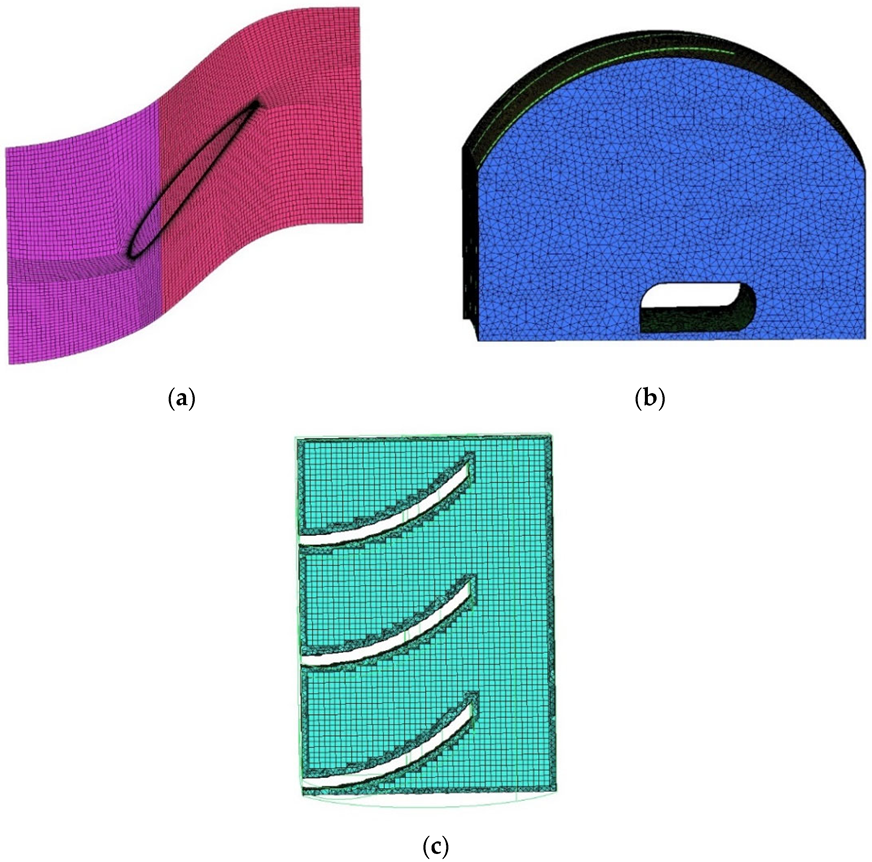
5.3. Meshing Details and Boundary Conditions

ICEM and Turbogrid were used to mesh the blades and the casing treatment. Block-structured grids were generated for bellmouth inlet/IGV/rotor/stator/outlet domains independently, while the casing treatment was discretized by structured and unstructured grids due to its complicated geometry. A view of the computational grids for the rotor and the casing treatment front and top views are shown in Figure 6.
The applied boundary conditions at the inlet are total temperature and total pressure. At the outlet, static pressure and mass flow were employed. For the calculation of maximum mass flow rate, static pressure was imposed at the outlet, while for the remaining operating points, the mass flow was gradually reduced.

5.4. Grid Independence Study

In order to assess the grid independence of the computations, the mesh density was increased toward the wall boundaries. Table 13 summarizes the details of five simulated meshes in addition to their mesh quality. Three monitor probes were placed in IGV, rotor, and stator domains to record static pressure. The locations of the numerical probes are shown in Figure 7. The recorded pressure by probe number 2 in the rotor was used to generate the pressure signals. The time-averaged pressure at monitor points 1, 2, and 3 changes slightly by refining the mesh. In addition, the comparison of pressure ratio shows that the pressure ratio almost remains constant, which shows that grid independence has been achieved. To save on unsteady computations, a medium grid type was utilized for the numerical computations.
40 time steps per a passing period (1520 time steps in a full rotation of the rotor) corresponding to a time step of 1.31579 × 10 5   s were selected for the simulations. The convergence of all the transient simulations was assessed by analyzing the time traces of static pressure and other parameters. Periodic signals were observed at the operating points away from the rotating stall and surge. Minimum numbers of one to two rotations were required to obtain periodic signals away from the instabilities. At in-stall and surge conditions, the periodicity of the signals in time breaks down. Following Gourdain [21], simulations at near stall and in-stall conditions were run for sufficient time to reduce the uncertainty associated with the results.

6. Validation of the Developed Model and the Predictions of Stall and Surge

Figure 3 demonstrates the influence of the number of stall cells on the total energy and the spectral entropy. Although the trends of these curves change toward lower mass flow rates, an exact criterion could not be specified to detect the stability limits based on the total energy and the entropy results alone. To resolve this problem, the statistical sum of square total SS (Total) is utilized in this section to unite the total energy/entropy curves into single curves. The sum of square total SS (Total) is mathematically defined as:
SS   Total = i = 1 k j = 1 n y i j y ¯ .. 2
where k is the number of treatments and n is the number of observations for treatment i.
y i j can take any total energy and spectral entropy values and y ¯ .. is the grand mean.
The SS (Total) of the total energy and the spectral entropy as a function of mass flow rate are shown in Figure 8. The total energy and the spectral entropy curves have been plotted on the same figure to show the correlation between them easily. As can be seen, the figure can be divided into four regions, namely A, B, C, and D. These regions coincide with the compressor stalling patterns as pre-stall, rotating stall, surge, and compressor failure, respectively. Region A is the region in which SS (Total) of the total energy and the spectral entropy reduce simultaneously. The spectral entropy reaches a local minimum at 1.95 kg/s while the total energy is still decreasing. This region is termed the pre-stall condition in which small disturbances are formed and expand with a reduction in mass flow. In region B, the total entropy reaches an inflection point at point A, and the total energy reaches a global minimum. In this region, the disturbances grow and reach a critical size and begin to move along the blade row. This region is termed the rotating stall. In region C, the total energy rises and attains a global maximum, while the total entropy reaches a new inflection point at B. In this region, noise and vibration are intensified due to increased secondary flow oscillations and surge initiates. The operation of the compressor in region D is termed the failure of the compressor since it follows surge, and the mass flow rate reaches very low.
The measurements for the experimental compressor indicated that rotating stall and surge for the configuration under study initiate at 1.95 kg/s and 1.52 kg/s, respectively [25,26]. The predictions of the onset of stall and surge based on the full-annulus approximation agree well with the experimental data, while the maximum error in predicting the onset of surge is 5.2%, which indicates the approximation of the full-annulus compressor is acceptable, as shown in Table 14.
The computed overall performance for SC (solid casing) and CT (casing treatment) is compared with the corresponding experimental results in Figure 9. As can be seen, a reasonable agreement exists between the numerical and the experimental results in terms of shape and value.
In summary, the full-annulus approximation model provides a reasonable estimation of stall inception and surge operating points, and due to its simplicity, it can be utilized to predict the multiblade instabilities in the preliminary design stage of a compressor. The main advantage of the current model is that the reconstruction of the full-annulus compressor and numerical simulations are computationally efficient since a single-passage simulation should be performed at a time. Having said that, despite the fact that the developed model has been validated with the available experimental data, the range of validity for other compressors should be investigated.

7. Conclusions

A full-annulus compressor was reconstructed conceptually and numerically to predict the stability limits for a low-pressure rise compressor that requires a full-annulus simulation due to limitations of conventional single-passage simulations and numerical error.
The following conclusions can be obtained:
  • The reconstruction of the full-annulus compressor based on the presence of disturbance including no disturbance, formation, and growth of disturbance and a systematic approach can be implemented successfully to reproduce pre-stall, in-stall, and surge flow regimes.
  • The reconstructed compressor coincides with the stalling patterns of actual compressors, including pre-stall, in-stall, surge, and breakdown conditions.
  • Spectral entropy and total energy due to secondary flow oscillations are effective indicators of rotating stall and surge instabilities.
  • Statistical ANOVA analysis and its sum of squares of total not only validate the results in terms of statistics but also can unite various results of total energy and spectral entropy.
  • The united results can show the correlation between total energy and spectral entropy and compressor operating conditions easily.
  • The predicted stall inception and surge operating points coincide well with the experimental data with minimal error.
  • The developed stability model can detect the multiblade rotating stall and surge instabilities and can be utilized in the preliminary design stage of a compressor.
  • The formation and disappearance of new frequencies provide a rough estimation of rotating stall.

Author Contributions

Conceptualization, N.M.N., M.A. and Y.A.; methodology, M.A., Y.A. and N.M.N.; software, Y.A.; validation, M.A., N.M.N. and Y.A.; formal analysis, Y.A.; investigation, Y.A. and M.A.; resources, Y.A.; writing—original draft preparation, Y.A.; writing—review and editing, Y.A.; supervision, M.A. All authors have read and agreed to the published version of the manuscript.

Funding

This research received no external funding.

Data Availability Statement

Not applicable.

Conflicts of Interest

The authors declare no conflict of interest.

Nomenclature

ANOVAAnalysis of variance
BPFBlade passing frequency
CTCasing treatment
ETotal energy
fProbability
FFTFast Fourier transform
f t Pressure signal
p i Probability distribution
SCSolid casing
SESpectral entropy
SSSum of square
X Power distribution
y ¯ Grand mean

References

  1. Day, I.J. Stall, surge and 75 years of research. J. Turbomach. 2016, 138, 1–16. [Google Scholar] [CrossRef]
  2. Cumpsty, N.A. Compressor Aerodynamics, 1st ed.; Longman Scientific & Technical: Essex, UK, 1989; pp. 359–362. [Google Scholar]
  3. Dixon, S.L.; Hall, C.A. Fluid Mechanics and Thermodynamics of Turbomachinery, 7th ed.; Elsevier: Oxford, UK, 2014; pp. 198–200. [Google Scholar]
  4. Stenning, A.; Kriebel, A. Stall Propagation in a Cascade of Aerofoils. Trans. ASME 1958, 80, 777–789. [Google Scholar]
  5. Stenning, A. Rotating Stall and Surge. J. Fluids Eng. 1980, 102, 14–20. [Google Scholar] [CrossRef]
  6. Greitzer, E.M. Review axial compressor stall phenomena. J. Fluids Eng. 1980, 102, 134–151. [Google Scholar] [CrossRef]
  7. Greitzer, E. Surge and Rotating Stall in Axial Flow Compressors—Part I: Theoretical Compression System Model. ASME J. Eng. Gas Turbines Power 1976, 98, 190–198. [Google Scholar] [CrossRef]
  8. Greitzer, E. Surge and Rotating Stall in Axial Flow Compressors—Part II: Experimental Results and Comparison with Theory. ASME J. Eng. Gas Turbines Power 1976, 98, 199–211. [Google Scholar] [CrossRef]
  9. Cumpsty, N.; Greitzer, E.M. A Simple Model for Compressor Stall Cell Propagation. J. Eng. Power 1982, 104, 170–176. [Google Scholar] [CrossRef]
  10. Moore, F. A Theory of Rotating Stall of Multistage Axial Compressors: Part I—Small Disturbances. ASME J. Eng. Gas Turbines Power 1984, 106, 313–320. [Google Scholar] [CrossRef]
  11. Moore, F. A Theory of Rotating Stall of Multistage Axial Compressors: Part II—Finite Disturbances. ASME J. Eng. Gas Turbines Power 1984, 106, 321–326. [Google Scholar] [CrossRef]
  12. Moore, F. A Theory of Rotating Stall of Multistage Axial Compressors: Part III—Limit Cycles. ASME J. Eng. Gas Turbines Power 1984, 106, 327–334. [Google Scholar] [CrossRef]
  13. Gogoi, A.; Verma, S.; Sane, S.K. A model for rotating stall and surge in axial flow compressors. In Proceedings of the 38th AIAA/ASME/SAE/ASEE Joint Propulsion Conference & Exhibit, Indianapolis, IN, USA, 7–10 July 2002. [Google Scholar]
  14. Benavides, E.M. On the Theoretical Calculation of the Stability Line of an Axial-flow Compressor Stage. Int. J. Turbo. Jet-Engines 2011, 28, 285–298. [Google Scholar] [CrossRef]
  15. Benavides, E.M.; Juste, G.L. Analytical Calculation of Stall-inception and Surge Points for an Axial-flow Compressor Rotor. Int. J. Turbo. JET-Engines 2012, 29, 243–257. [Google Scholar] [CrossRef]
  16. Vo, H.D.; Tan, C.S.; Greitzer, E.M. Criteria for spike initiated rotating stall. J. Turbomach. 2008, 130, 011023-1-9. [Google Scholar] [CrossRef]
  17. Lu, X.; Chu, C.; Zhu, J.; Wu, Y. Mechanism of the interaction between casing treatment and tip leakage flow in a subsonic axial compressor. In Proceedings of the GT2006 ASME Turbo Expo ASME Paper 2006 Power for Land Sea and Air, Barcelona, Spain, 8–11 May 2006. [Google Scholar]
  18. Khaleghi, H. Effect of axial skewed slot casing treatment in a transonic fan. Proc. IMechE Part G J. Aerosp. Eng. 2017, 231, 2646–2653. [Google Scholar] [CrossRef]
  19. Zhou, X.; Zhao, Q. Investigation on Axial Effect of Slot Casing Treatment in a Transonic Compressor. Appl. Therm. Eng. 2017, 126, 53–69. [Google Scholar] [CrossRef]
  20. Hwang, Y.; Kang, S.H. Numerical study on the effects of casing treatment on unsteadiness of tip leakage flow in an axial compressor. In Proceedings of the ASME Turbo Expo 2012 GT2012, Copenhagen, Denmark, 11–15 June 2012. [Google Scholar]
  21. Gourdain, N.; Burguburu, S.; Leboeuf, F.; Michon, G.J. Simulation of rotating stall in a whole stage of an axial compressor. Comput. Fluids 2010, 39, 1644–1655. [Google Scholar] [CrossRef]
  22. Cornelius, C.; Biesinger, T.; Galpin, P.; Braune, A. Experimental and computational analysis of a multistage axial compressor including stall prediction by steady and transient CFD methods. J. Turbomach. 2014, 136, 1–12. [Google Scholar] [CrossRef]
  23. Day, I.J.; Greitzer, E.M.; Cumpsty, N.A. Prediction of compressor performance in rotating stall. J. Eng. Power 1978, 100, 1–12. [Google Scholar] [CrossRef]
  24. Tan, C.S.; Day, I.; Morris, S.; Wadia, A. Spike-type compressor stall inception, detection, and control. Annu. Rev. Fluid Mech. 2010, 42, 275–300. [Google Scholar] [CrossRef]
  25. Akhlaghi, M. Application of a Vane-Recessed Tubular-Passage Casing Treatment to a Multistage Axial-Flow Compressor. Ph.D. Thesis, University of Cranfield, Cranfield, UK, 2001. [Google Scholar]
  26. Akhlaghi, M.; Elder, R.L.; Ramsden, K.W. Effects of a vane-recessed tubular-passage passive stall control technique on a multistage, low-speed, axial-flow compressor: Results of tests on the first stage with the rear stages removed. In Proceedings of the ASME Turbo Expo 2003 Power for Land Sea and Air, Atlanta, GE, USA, 16–19 June 2003. [Google Scholar]
Figure 1. Stall cell formation and propagation.
Machines 10 00706 g001
Figure 2. Reconstruction of the full-annulus compressor.
Machines 10 00706 g002
Figure 3. Total energy and spectral entropy versus mass flow rate.
Machines 10 00706 g003
Figure 4. Frequency versus mass flow rate.
Machines 10 00706 g004
Figure 5. Layout of the test rig [25,26].
Machines 10 00706 g005
Figure 6. Computational grids for (a) rotor blade, (b) casing treatment front view, and (c) casing treatment top view.
Machines 10 00706 g006
Figure 7. Locations of the numerical probes 1, 2, and 3.
Machines 10 00706 g007
Figure 8. Sum of squares total of total energy and spectral entropy versus mass flow rate.
Machines 10 00706 g008
Figure 9. Pressure ratio and isentropic efficiency versus mass flow rate.
Machines 10 00706 g009
Table 1. Simulated mass flow rates.
CodeMass Flow in One Passage (kg/s)
A0.0635306
B0.0617871
C0.0559985
D0.0540200
E0.0504862
F0.0453949
G0.0424009
H0.0406331
I0.0382239
J0.0266138
K0.0203937
Table 2. Combinations of mass flow rates for one stall cell.
RunTotal Mass Flow Rate (kg/s)Combination Code
12.4141628AAAAAAAAAAAAAAAAAAAAAAAAAAAAAAAAAAAAAA
22.4106758AAAAAAAAAAAAAAAAAABBAAAAAAAAAAAAAAAAAA
32.3956116AAAAAAAAAAAAAAAAABCCBAAAAAAAAAAAAAAAAA
42.3765904AAAAAAAAAAAAAAAABCDDCBAAAAAAAAAAAAAAAA
52.35050AAAAAAAAAAAAAAABCDEEDCBAAAAAAAAAAAAAAA
62.3142302AAAAAAAAAAAAAABCDEFFEDCBAAAAAAAAAAAAAA
72.2719708AAAAAAAAAAAAABCDEFGGFEDCBAAAAAAAAAAAAA
82.2261758AAAAAAAAAAAABCDEFGHHGFEDCBAAAAAAAAAAAA
92.1755624AAAAAAAAAAABCDEFGHIIHGFEDCBAAAAAAAAAAA
102.1017288AAAAAAAAAABCDEFGHIJJIHGFEDCBAAAAAAAAAA
112.015455AAAAAAAAABCDEFGHIJKKJIHGFEDCBAAAAAAAAA
121.9291812AAAAAAAABCDEFGHIJKKKKJIHGFEDCBAAAAAAAA
131.8429074AAAAAAABCDEFGHIJKKKKKKJIHGFEDCBAAAAAAA
141.7566336AAAAAABCDEFGHIJKKKKKKKKJIHGFEDCBAAAAAA
151.6703598AAAAABCDEFGHIJKKKKKKKKKKJIHGFEDCBAAAAA
161.584086AAAABCDEFGHIJKKKKKKKKKKKKJIHGFEDCBAAAA
171.4978122AAABCDEFGHIJKKKKKKKKKKKKKKJIHGFEDCBAAA
181.4115384AABCDEFGHIJKKKKKKKKKKKKKKKKJIHGFEDCBAA
191.3252646ABCDEFGHIJKKKKKKKKKKKKKKKKKKJIHGFEDCBA
201.2389908BCDEFGHIJKKKKKKKKKKKKKKKKKKKKJIHGFEDCB
211.156204CDEFGHIJKKKKKKKKKKKKKKKKKKKKKKJIHGFEDC
221.0849944DEFGHIJKKKKKKKKKKKKKKKKKKKKKKKKJIHGFED
231.0177418EFGHIJKKKKKKKKKKKKKKKKKKKKKKKKKKJIHGFE
240.9575568FGHIJKKKKKKKKKKKKKKKKKKKKKKKKKKKKJIHGF
250.9075544GHIJKKKKKKKKKKKKKKKKKKKKKKKKKKKKKKJIHG
260.86354HIJKKKKKKKKKKKKKKKKKKKKKKKKKKKKKKKKJIH
270.8230612IJKKKKKKKKKKKKKKKKKKKKKKKKKKKKKKKKKKJI
280.7874008JKKKKKKKKKKKKKKKKKKKKKKKKKKKKKKKKKKKKJ
290.7749606KKKKKKKKKKKKKKKKKKKKKKKKKKKKKKKKKKKKKK
Table 3. Combinations of mass flow rates for two stall cells.
RunTotal Mass Flow Rate (kg/s)Combination Code
12.4141628AAAAAAAAAAAAAAAAAAAAAAAAAAAAAAAAAAAAAA
22.4071888AAAAAAAABBAAAAAAAAAAAAAAAAAABBAAAAAAAA
32.3770604AAAAAAABCCBAAAAAAAAAAAAAAAABCCBAAAAAAA
42.339018AAAAAABCDDCBAAAAAAAAAAAAAABCDDCBAAAAAA
52.2868404AAAAABCDEEDCBAAAAAAAAAAAABCDEEDCBAAAAA
62.2142976AAAABCDEFFEDCBAAAAAAAAAABCDEFFEDCBAAAA
72.1297788AAABCDEFGGFEDCBAAAAAAAABCDEFGGFEDCBAAA
82.0381888AABCDEFGHHGFEDCBAAAAAABCDEFGHHGFEDCBAA
91.936962ABCDEFGHIIHGFEDCBAAAABCDEFGHIIHGFEDCBA
101.7892948BCDEFGHIJJIHGFEDCBAABCDEFGHIJJIHGFEDCB
111.6202342CDEFGHIJKKJIHGFEDCBBCDEFGHIJKKJIHGFEDC
121.4662378DEFGHIJKKKKJIHGFEDCCDEFGHIJKKKKJIHGFED
131.3277756EFGHIJKKKKKKJIHGFEDDEFGHIJKKKKKKJIHGFE
141.200338FGHIJKKKKKKKKJIHGFEEFGHIJKKKKKKKKJIHGF
151.0901506GHIJKKKKKKKKKKJIHGFFGHIJKKKKKKKKKKJIHG
160.9961338HIJKKKKKKKKKKKKJIHGGHIJKKKKKKKKKKKKJIH
170.9116406IJKKKKKKKKKKKKKKJIHHIJKKKKKKKKKKKKKKJI
180.8355014JKKKKKKKKKKKKKKKKJIIJKKKKKKKKKKKKKKKKJ
190.7874008KKKKKKKKKKKKKKKKKKJJKKKKKKKKKKKKKKKKKK
200.7749606KKKKKKKKKKKKKKKKKKKKKKKKKKKKKKKKKKKKKK
Table 4. Combinations of mass flow rates for three stall cells.
RunTotal Mass Flow Rate (kg/s)Combination Code
12.4141628AAAAAAAAAAAAAAAAAAAAAAAAAAAAAAAAAAAAAA
22.4037018AAAAABBAAAAAAAAAAABBAAAAAAAAAAABBAAAAA
32.3585092AAAABCCBAAAAAAAAABCCBAAAAAAAAABCCBAAAA
42.3014456AAABCDDCBAAAAAAABCDDCBAAAAAAABCDDCBAAA
52.2231792AABCDEEDCBAAAAABCDEEDCBAAAAABCDEEDCBAA
62.114365ABCDEFFEDCBAAABCDEFFEDCBAAABCDEFFEDCBA
71.9875868BCDEFGGFEDCBABCDEFGGFEDCBABCDEFGGFEDCB
81.8571758CDEFGHHGFEDCBCDEFGHHGFEDCBCDEFGHHGFEDC
91.738951DEFGHIIHGFEDCDEFGHIIHGFEDCDEFGHIIHGFED
101.5705568EFGHIJJIHGFEDEFGHIJJIHGFEDEFGHIJJIHGFE
111.3953744FGHIJKKJIHGFEFGHIJKKJIHGFEFGHIJJJJIHGF
121.2227444GHIJKKKKJIHGFGHIJKKKKJIHGFGHIJKKKKJIHG
131.0847132HIJKKKKKKJIHGHIJKKKKKKJIHGHIJKKKKKKJIH
140.9597412IJKKKKKKKKJIHIJKKKKKKKKJIHIJKKKKKKKKJI
150.8479416JKKKKKKKKKKJIJKKKKKKKKKKJIJKKKKKKKKKKJ
160.7874008KKKKKKKKKKKKJKKKKKKKKKKKKJKKKKKKKKKKKK
170.7749606KKKKKKKKKKKKKKKKKKKKKKKKKKKKKKKKKKKKKK
Table 5. Combinations of mass flow rates for four stall cells.
RunTotal Mass Flow Rate (kg/s)Combination Code
12.4141628AAAAAAAAAAAAAAAAAAAAAAAAAAAAAAAAAAAAAA
22.4002148AAAABBAAAAAAAABBAAAAAAAABBAAAAAAAABBAA
32.339958AAABCCBAAAAAABCCBAAAAAABCCBAAAAAABCCBA
42.2638732AABCDDCBAAAABCDDCBAAAABCDDCBAAAABCDDCB
52.1612615ABCDEEDCBAABCDEEDCBAABCDEEDCBAABCDEEDC
62.023708BCDEFFEDCBBCDEFFEDCBBCDEFFEDCBBCDEFFED
71.8763855CDEFGGFEDCCDEFGGFEDCCDEFGGFEDCCDEFGGFE
81.7589746DEFGHHGFEDDEFGHHGFEDDEFGHHGFEDDEFGHHGF
91.6412309EFGHIIHGFEEFGHIIHGFEEFGHIIHGFEEFGHIIHG
101.458337FGHIJJIHGFFGHIJJIHGFFGHIJJIHGFFGHIJJIH
111.2630892GHIJKKJIHGGHIJKKJIHGGHIJKKJIHGGHIJKKJI
121.0912086HIJKKKKJIHHIJKKKKJIHHIJKKKKJIHHIJKKKKJ
130.9433127IJKKKKKKJIIJKKKKKKJIIJKKKKKKJIIJKKKKKK
140.8185013JKKKKKKKKJJKKKKKKKKJJKKKKKKKKJJKKKKKKK
150.7749606KKKKKKKKKKKKKKKKKKKKKKKKKKKKKKKKKKKKKK
Table 6. Combinations of mass flow rates for five stall cells.
RunTotal Mass Flow Rate (kg/s)Combination Code
12.4141628AAAAAAAAAAAAAAAAAAAAAAAAAAAAAAAAAAAAAA
22.3967278AAABBAAAAAABBAAAAAABBAAAAAABBAAAAAABBA
32.3214068AABCCBAAAABCCBAAAABCCBAAAABCCBAAAABCCB
42.2280443ABCDDCBAABCDDCBAABCDDCBAABCDDCBAABCDDC
52.1051324BCDEEDCBBCDEEDCBBCDEEDCBBCDEEDCBBCDEED
61.9489775CDEFFEDCCDEFFEDCCDEFFEDCCDEFFEDCCDEFFE
71.8185138DEFGGFEDDEFGGFEDDEFGGFEDDEFGGFEDDEFGGF
81.6932699EFGHHGFEEFGHHGFEEFGHHGFEEFGHHGFEEFGHHG
91.5787322FGHIIHGFFGHIIHGFFGHIIHGFFGHIIHGFFGHIIH
101.395683GHIJJIHGGHIJJIHGGHIJJIHGGHIJJIHGGHIJJI
111.179788HIJKKJIHHIJKKJIHHIJKKJIHHIJKKJIHHIJKKJ
120.9914133IJKKKKJIIJKKKKJIIJKKKKJIIJKKKKJIIJKKKK
130.8309415JKKKKKKJJKKKKKKJJKKKKKKJJKKKKKKJJKKKKK
140.7749606KKKKKKKKKKKKKKKKKKKKKKKKKKKKKKKKKKKKKK
Table 7. Combinations of mass flow rates for six stall cells.
RunTotal Mass Flow Rate (kg/s)Combination Code
12.4141628AAAAAAAAAAAAAAAAAAAAAAAAAAAAAAAAAAAAAA
22.3932408AABBAAAABBAAAABBAAAABBAAAABBAAAABBAAAA
32.3011121ABCCBAABCCBAABCCBAABCCBAABCCBAABCCBAAB
42.1794528BCDDCBBCDDCBBCDDCBBCDDCBBCDDCBBCDDCBBC
52.0360749CDEEDCCDEEDCCDEEDCCDEEDCCDEEDCCDEEDCCD
61.9033194DEFFEDDEFFEDDEFFEDDEFFEDDEFFEDDEFFEDDE
71.7552651EFGGFEEFGGFEEFGGFEEFGGFEEFGGFEEFGGFEEF
81.6289426FGHHGFFGHHGFFGHHGFFGHHGFFGHHGFFGHHGFFG
91.5381288GHIIHGGHIIHGGHIIHGGHIIHGGHIIHGGHIIHGGH
101.3445066HIJJIHHIJJIHHIJJIHHIJJIHHIJJIHHIJJIHHI
111.0876145IJKKJIIJKKJIIJKKJIIJKKJIIJKKJIIJKKJIIJ
120.8558219JKKKKJJKKKKJJKKKKJJKKKKJJKKKKJJKKKKJJK
130.7749606KKKKKKKKKKKKKKKKKKKKKKKKKKKKKKKKKKKKKK
Table 8. Combinations of mass flow rates for seven stall cells.
RunTotal Mass Flow Rate (kg/s)Combination Code
12.4141628AAAAAAAAAAAAAAAAAAAAAAAAAAAAAAAAAAAAAA
22.3897538AAABBAAABBAAABBAAABBAAABBAAABBAAABBAAA
32.2843044AABCCBABCCBABCCBABCCBABCCBABCCBABCCBAA
42.161617ABCDDCBCDDCBCDDCBCDDCBCDDCBCDDCBCDDCBA
52.034649BCDEEDCDEEDCDEEDCDEEDCDEEDCDEEDCDEEDCB
61.8864924CDEFFEDEFFEDEFFEDEFFEDEFFEDEFFEDEFFEDC
71.7410708DEFGGFEFGGFEFGGFEFGGFEFGGFEFGGFEFGGFED
81.6266076EFGHHGFGHHGFGHHGFGHHGFGHHGFGHHGFGHHGFE
91.533995FGHIIHGHIIHGHIIHGHIIHGHIIHGHIIHGHIIHGF
101.3175944GHIJJIHIJJIHIJJIHIJJIHIJJIHIJJIHIJJIHG
111.0451624HIJKKJIJKKJIJKKJIJKKJIJKKJIJKKJIJKKJIH
120.8603818IJKKKKJKKKKJKKKKJKKKKJKKKKJKKKKJKKKKJI
130.7874008JKKKKKKKKKKKKKKKKKKKKKKKKKKKKKKKKKKKKJ
140.7749606KKKKKKKKKKKKKKKKKKKKKKKKKKKKKKKKKKKKKK
Table 9. Combinations of mass flow rates for eight stall cells.
RunTotal Mass Flow Rate (kg/s)Combination Code
12.4141628AAAAAAAAAAAAAAAAAAAAAAAAAAAAAAAAAAAAAA
22.3862668AAAABBAABBAABBAABBAABBAABBAABBAABBAAAA
32.2657532AAABCCBBCCBBCCBBCCBBCCBBCCBBCCBBCCBAAA
42.1379926AABCDDCCDDCCDDCCDDCCDDCCDDCCDDCCDDCBAA
52.03ABCDEEDDEEDDEEDDEEDDEEDDEEDDEEDDEEDCBA
61.8777088BCDEFFEEFFEEFFEEFFEEFFEEFFEEFFEEFFEDCB
71.73CDEFGGFFGGFFGGFFGGFFGGFFGGFFGGFFGGFEDC
81.63DEFGHHGGHHGGHHGGHHGGHHGGHHGGHHGGHHGFED
91.538276EFGHIIHHIIHHIIHHIIHHIIHHIIHHIIHHIIHGFE
101.294261FGHIJJIIJJIIJJIIJJIIJJIIJJIIJJIIJJIHGF
110.9946358GHIJKKJJKKJJKKJJKKJJKKJJKKJJKKJJKKJIHG
120.86354HIJKKKKKKKKKKKKKKKKKKKKKKKKKKKKKKKKJIH
130.8230612IJKKKKKKKKKKKKKKKKKKKKKKKKKKKKKKKKKKJI
140.7874008JKKKKKKKKKKKKKKKKKKKKKKKKKKKKKKKKKKKKJ
150.7749606KKKKKKKKKKKKKKKKKKKKKKKKKKKKKKKKKKKKKK
Table 10. ANOVA analysis for the total energy.
Source of VariationSum of SquareDegrees of FreedomMean SquaresFp-Value
Treatments5.22 × 1011341.53 × 101038.280.000
Error9.83 × 10102454.01 × 108
Total6.20 × 1011279
Table 11. ANOVA analysis for the spectral entropy.
Source of VariationSum of SquareDegrees of FreedomMean SquaresFp-Value
Treatments9.9265340.2919627.570.000
Error2.59472450.01059
Total12.5212279
Table 12. Specification of the experimental Peregrine compressor.
ParameterValue
Number of IGV blades34
Number of rotor blades38
Number of stator blades37
Rotor blade tip diameter405 mm
Rotor blade hub diameter284.4 mm
Tip clearance0.7 mm
Hub-to-tip ratio0.7
Rotor blade chord30.5 mm
Rotor blade aspect ratio2.0
Table 13. Effect of mesh size on time-averaged pressure and mesh quality.
ParameterValue
Grid NameCoarse-1Coarse-2MediumFine-1Fine-2
Total number of nodes791,7131,101,8032,224,4435,085,83510,565,038
Time-averaged pressure at monitor point 1 (Pa)100,860100,859100,851100,855100,856
Time-averaged pressure at monitor point 2 (Pa)101,444101,453101,459101,471101,472
Time-averaged pressure at monitor point 3 (Pa)101,879101,898101,947101,973102,002
Time-averaged pressure ratio1.0031.0031.0041.0041.004
Mesh statisticsMin. angle23.823.921.920.819.4
Max. aspect ratio679559427346220
Table 14. Comparison of the stall and surge inception points between predictions and experiments.
Operating PointPredictionExperimental DataError
Stall inception1.951.950
Surge inception1.61.525.2%
Publisher’s Note: MDPI stays neutral with regard to jurisdictional claims in published maps and institutional affiliations.

