A Few-Shot Learning-Based Crashworthiness Analysis and Optimization for Multi-Cell Structure of High-Speed Train

Abstract

Due to the requirement of significant manpower and material resources for the crashworthiness tests, various modelling approaches are utilized to reduce these costs. Despite being informative, finite element models still have the disadvantage of being time-consuming. A data-driven model has recently demonstrated potential in terms of computational efficiency, but it is also accompanied by challenges in collecting an amount of data. Few-shot learning is a perspective approach in addressing the problem of insufficient data in engineering. In this paper, using a novel hybrid data augmentation method, we investigate a deep-learning-based few-shot learning approach to evaluate and optimize the crashworthiness of multi-cell structures. Innovatively, we employ wide and deep neural networks to develop a surrogate model for multi-objective optimization. In comparison with the original results, the optimized result of the multi-cell structure demonstrates that the mean crushing force (F_m) and specific energy absorption (SEA) are increased by 17.1% and 30.1%, respectively, the mass decreases by 4.0%, and the optimized structure offers a significant improvement in design space. Overall, this proposed method exhibits great potential in relation to the crashworthiness analysis and optimization for multi-cell structures of the high-speed train.

1. Introduction

Due to the severe casualties and property losses in railway collision accidents, crashworthiness analysis and optimization have received great attention. Researchers have investigated collision dynamic performance mainly through three methods: (i) Crash test [1]—while the tests have the advantage of being reliable, the cost and labor associated with them is significant; (ii) Finite element (FE) simulation [2,3]—the FE simulation could reduce human labor and costs by simulating the geometry, material properties, and connections of each component; however, they are still faced with complicated models and time-consuming calculations; (iii) Theoretical approach [4]—this approach is developed using simplified super folding element (SAFE) theory, which generally requires rich experience, and professional knowledge of mechanics and mathematics.

Recently, Machine Learning, as a novel developed data-driven approach, has yielded significant improvement in terms of efficiency, and has been extensively used in the engineering area to simulate highly nonlinear interactions between inputs and outputs of crash dynamics. For instance, the stable behavior prediction of a thin-walled box [5], the force–displacement characteristics analysis of train crashes [6,7], the integrated dynamic response prediction of automobile crashes [8], and the crash process estimation of vehicle-barrier frontal crashes [9] were all analyzed by Karimi et al. [10]. These approaches could directly analyze and predict crash dynamics characteristics using the trained model, which has significantly increased computing efficiency. However, these approaches generally required an amount of data for training the data-driven model, leading to the relatively high cost of collecting data.

In order to address these issues, a few-shot learning algorithm based on prior knowledge has been proposed, which can rapidly generalize new tasks with only a few samples of supervised information. Currently, these studies of few-shot learning algorithms can be mainly categorized into three perspectives: (i) data, which enhances the supervised experience with prior knowledge; (ii) model, which reduces the size of the hypothesis space based on prior knowledge; and (iii) algorithm, which searches for the best hypothesis in a given hypothesis space based on prior experience [11]. With the development of the few-shot learning algorithm, there are many applications in engineering, such as disease classification [12], fault diagnosis [13], and image interpretation [14]. Thus, the few-shot learning method would have a better perspective when applied in crashworthiness analysis and optimization.

Multi-cell structures, with the advantage of being lightweight, could dissipate more crash energy and could reduce the impact pressures of the passengers during the collision process than single-cell structures [15,16]. Researchers have gradually adopted multi-cell structures instead of single-cell structures to protect the passengers against impact caused by railway collision accidents. For decades, the energy absorption behavior of thin-walled structures has been investigated under different loading conditions, including axial [17,18,19], lateral [20,21,22], oblique [23,24,25], and bending [26,27,28]. Among them, the axial crushing mode is the most efficient for energy absorption since the majority of the structure is plastic material [29]. Therefore, it is essential to study the collision dynamic performance of multi-cell structures under axial impact.

In the present study, we propose a few-shot learning-based approach to analyze and optimize the crashworthiness for the multi-cell structure of a high-speed train (refer to Figure 1) under the axial impact. The framework of our study involved the following: (i) data augmentation—the generalized data generation from three crashworthiness analysis methods of Simplified Super Folding Element (SSFE) theory, finite element (FE) simulation, and tests; (ii) modelling—the deep learning model of a wide and deep neural network is trained to accurately estimate the nonlinear relationship between the structure parameters (e.g., wall thickness and cell length) and the crashworthiness performance (e.g., mean crushing force and specific energy absorption); (iii) multi-objective optimization—a multi-objective optimization based on the deep learning-based few-shot learning model is carried out using the Non-dominated Sorting Genetic Algorithm-III (NSGA-III) to seek the optimum design space.

2. Materials and Methods

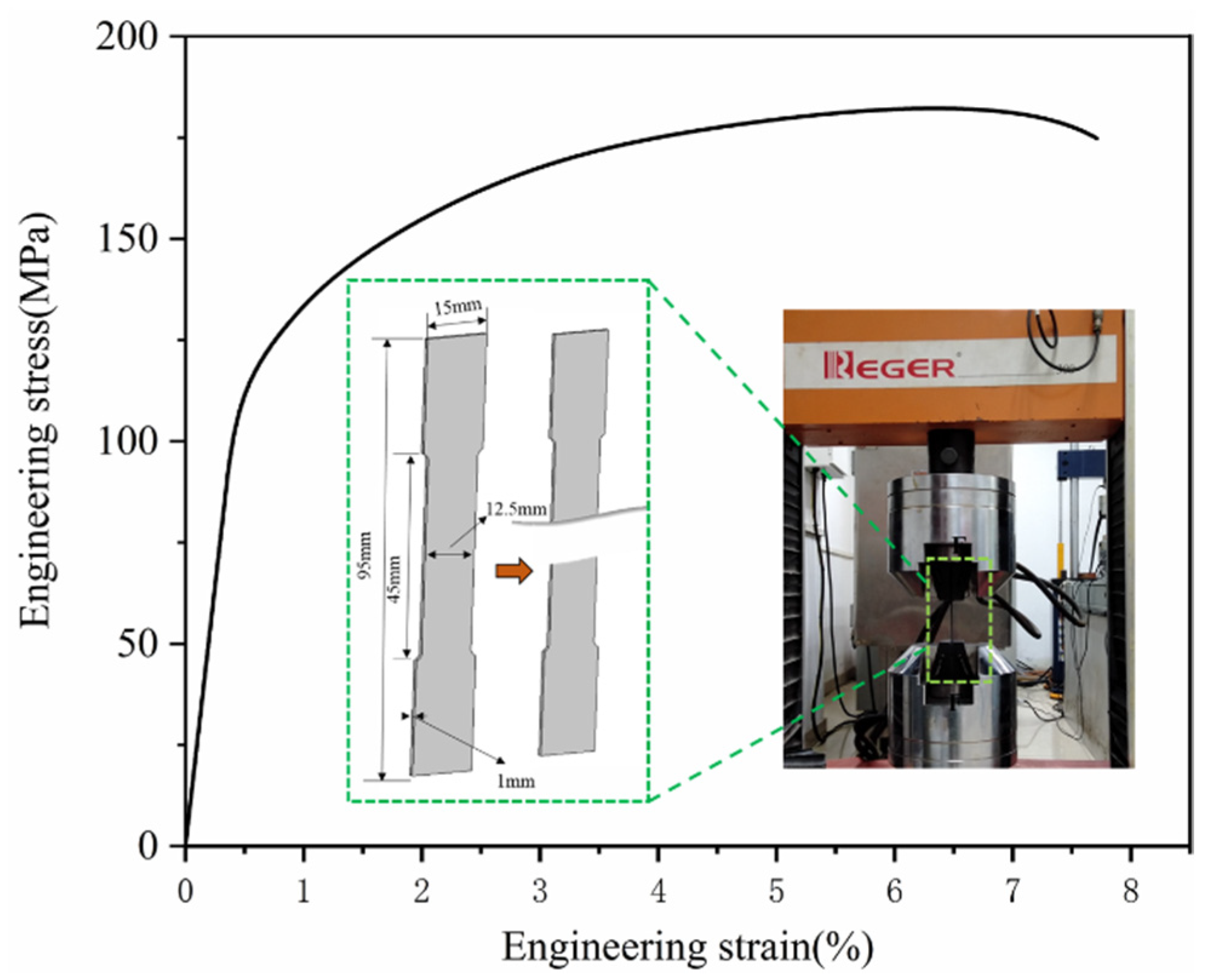
2.1. Materials

In the present study, a honeycomb composite structure with five holes using an octagonal tube will be utilized as an energy absorber structure for the high-speed train. As depicted in Figure 2, the cell wall length a, wall-length b, cell wall length c, and thickness t of the multi-cell thin-walled structure are 56, 56, 51, and 5 mm, respectively, and the angle of the beveled edge to the side is 150°, the cross-section dimension H × W of the multi-cell structure is 280 × 245 mm and the length L of the multi-cell-structure is 500 mm [30,31].

2.1.1. Theoretical Analysis

For multi-cell structures under axial crushing load, the mean crushing force (F_m) and the specific energy absorption (SEA) can be calculated using the simplified super folding element theory (SSFE) [4]. According to the principle of conservation of energy, the energy absorption equation for the multi-cell structure of the high-speed train could be expressed as follows:

$$F_{\mathrm{m}}L=\frac{1}{\eta }\left(E_{\mathrm{b}}+E_{\mathrm{m}}\right),$$

(1)

where F, L, E_b, E_m and η are the mean crushing force, folding wavelength, bending deformation energy, film deformation energy, and the effective impact distance coefficient, respectively.

• Film deformation energy: The film deformation energy E_m of each flange plate can be calculated by integrating the triangular cells of a folded wavelength.

  $$E_{\mathrm{m}}={{\displaystyle \int }}_s{\sigma }_{0}t\mathrm{d}s=\frac{1}{8}{\sigma }_{0}t{L}^2=\frac{1}{2}{M}_0\frac{L^2}{t},$$

  (2)

  where $M_0=\frac{{\sigma }_0{t}^2}{4}$. An energy equivalent stress σ₀ can be used to approximate the flow stress for power-law hardening materials

  $${\sigma }_0=\sqrt{\frac{{\sigma }_y{\sigma }_u}{1+n}},$$

  (3)

  where ${\sigma }_y$, ${\sigma }_u$ and n denote the yield strength, the ultimate strength of the material, and the exponent of the power-law, respectively. Given that a plate’s function is similar to that of a rectangular thin-film unit, the deformation energy of a thin-film unit is twice that of a plate.

  $$E_{\mathrm{m}}^{{90}^{\circ }}=2E_{\mathrm{m}}=M_0\frac{L^2}{t},$$

  (4)

Then the deformation energy of the V-shaped film (Figure 2a) can be determined.

$$E_{\mathrm{m}}^V=\frac{E_{\mathrm{m}}^{{90}^{\circ }}}{\cos \gamma }=M_0\frac{L^2}{\mathrm{t}\mathrm{tcos}{15}^{\circ }},$$

(5)

As shown in Figure 2, the Y-I unit can be regarded as a combination of the V-shaped unit (Figure 2c) and an additional plate. A Y-II unit can be viewed as a unit composed of a right-angle unit and an additional plate, and its deformation energy can be determined.

$$E_{\mathrm{m}}^{\mathrm{add}}=2M_0\frac{L^2}{t}\tan \left(\frac{\phi }{2}\right),$$

(6)

Accordingly, the film deformation energy of Y-I and Y-II units can be divided as follows:

$$E_{\mathrm{m}}^{\mathrm{Y}-\mathrm{I}}=M_0\frac{L^2}{t}\left(\frac{1}{\cos {15}^{\circ }}+2\tan {60}^{\circ }\right),$$

(7)

$$E_{\mathrm{m}}^{\mathrm{Y}-\mathrm{II}}=M_0\frac{L^2}{t}\left(1+2\tan {60}^{\circ }\right),$$

(8)

• Bending deformation energy: Using the SSFE theory, where buckling wavelength L and wall thickness t are assumed to be constant, we can divide the energy absorption region of each corner unit into a thin film deformation zone and a bending deformation zone. For each of the flange plates, bending deformation energy is calculated as follows:

  $$E_{\mathrm{b}}={{\displaystyle \sum }}_{i=1}^3{M}_0{\theta }_{i}c=2\pi M_0{B}_0,$$

  (9)

  where c, B₀ and M₀ is the side length, the sum lengths of the corner cell wall and the plastic bending moment of the flange plate, respectively; the four rotation angle values θ_i at the bent strand are π/2.
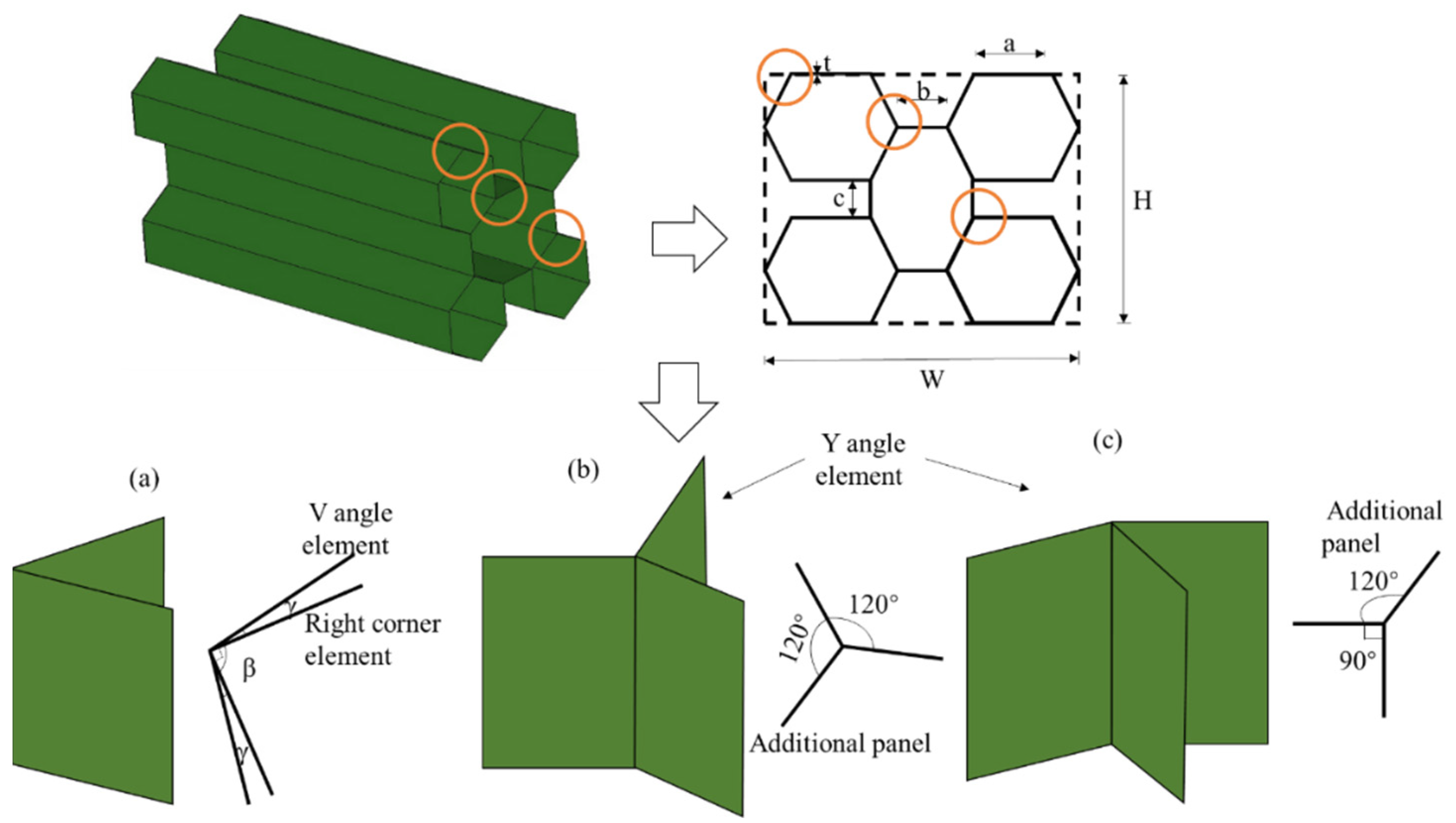
• Mean crushing forces: Five-cell structures with the cross-section configuration honeycomb tubes consist of 16 V-shaped elements, 4 Y-I-shaped elements, and 4 Y-II-shaped elements. We can then substitute Equations (5) and (7)–(9) into Equation (1) to obtain Equation (10).

  $$F_{\mathrm{m}}\mathrm{L}\eta =E_{\mathrm{b}3}+16E_{\mathrm{m}}^{\mathrm{V}}+4E_{\mathrm{m}}^{\mathrm{Y}-\mathrm{I}}+4E_{\mathrm{m}}^{\mathrm{Y}-\mathrm{II}},$$

  (10)

A mean crushing force can be calculated using Equation (11).

$$F_{\mathrm{m}}=\frac{\pi M_0{B}_3}{\eta H}+\frac{M_{0}H}{\eta \mathrm{t}}\left(4+\frac{20}{\cos {15}^{\circ }}+16\tan {60}^{\circ }\right)=7.24{\pi }^{0.5}{B}^{0.5}{t}^{1.5}{\sigma }_0,$$

(11)

A thin-walled structure might experience an axial impact load that is affected by its dynamic impact velocity. According to the literature [32], dynamic impact loads are usually bigger than equivalent quasi-static loads, and the dynamic increase coefficient λ is 1.2~1.5, which is proportional to the dynamic impact velocity (although other factors may affect the coefficient’s value, which is not considered in this study). Specifically, the initial velocity in this study is 10 m/s and the dynamic increase coefficient λ is set to 1.2. Accordingly, the revised mean crushing force of the multi-cell structure can be obtained as Equation (12).

$$F_{\mathrm{m}}=\lambda P_{\mathrm{m}3}=1.2\times 7.24{\pi }^{0.5}{B}^{0.5}{t}^{1.5}{\sigma }_0=8.688{\pi }^{0.5}{B}^{0.5}{t}^{1.5},$$

(12)

In addition, a lightweight mass and efficient energy absorption determine the energy absorption capacity of the multi-cell structure per mass unit. Thus, a multi-cell structure can be designed to improve crashworthiness by taking into account the energy that is absorbed per unit mass of the thin-walled component. This can be represented by Equation (13). According to the study by Abramowicz [33,34], there is a crush distance of around 70–75% of the wavelength L, so we can assume the value of 0.62 in the following derivation considering the engineering noise.

$$F_{\mathrm{m}}=\lambda P_{\mathrm{m}3}=1.2\times 7.24{\pi }^{0.5}{B}^{0.5}{t}^{1.5}{\sigma }_0=8.688{\pi }^{0.5}{B}^{0.5}{t}^{1.5},$$

(13)

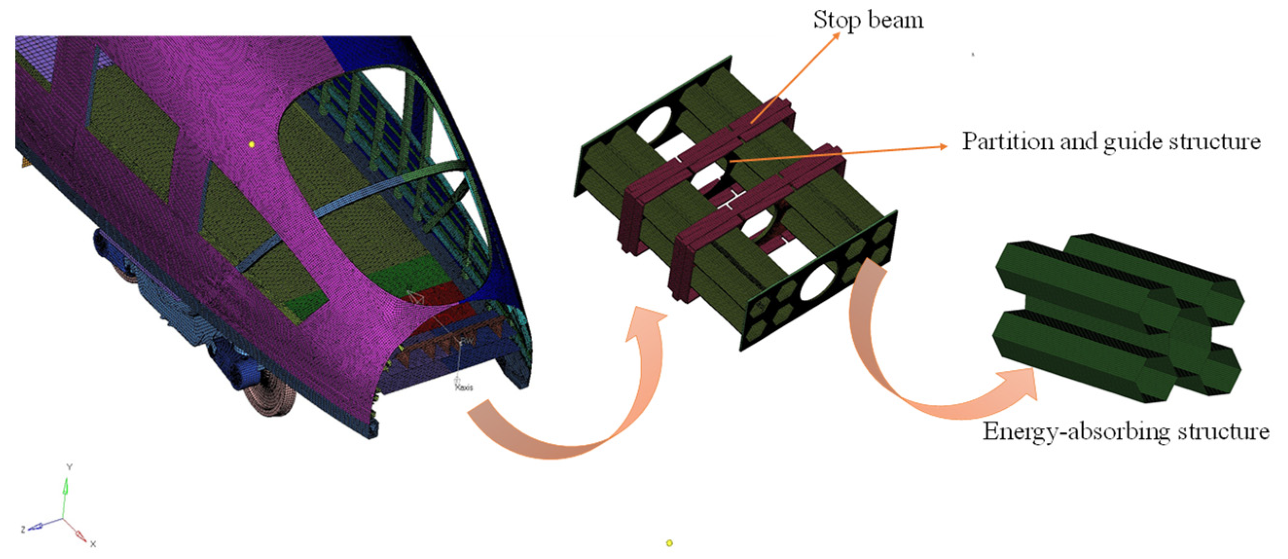
2.1.2. Finite Element Model

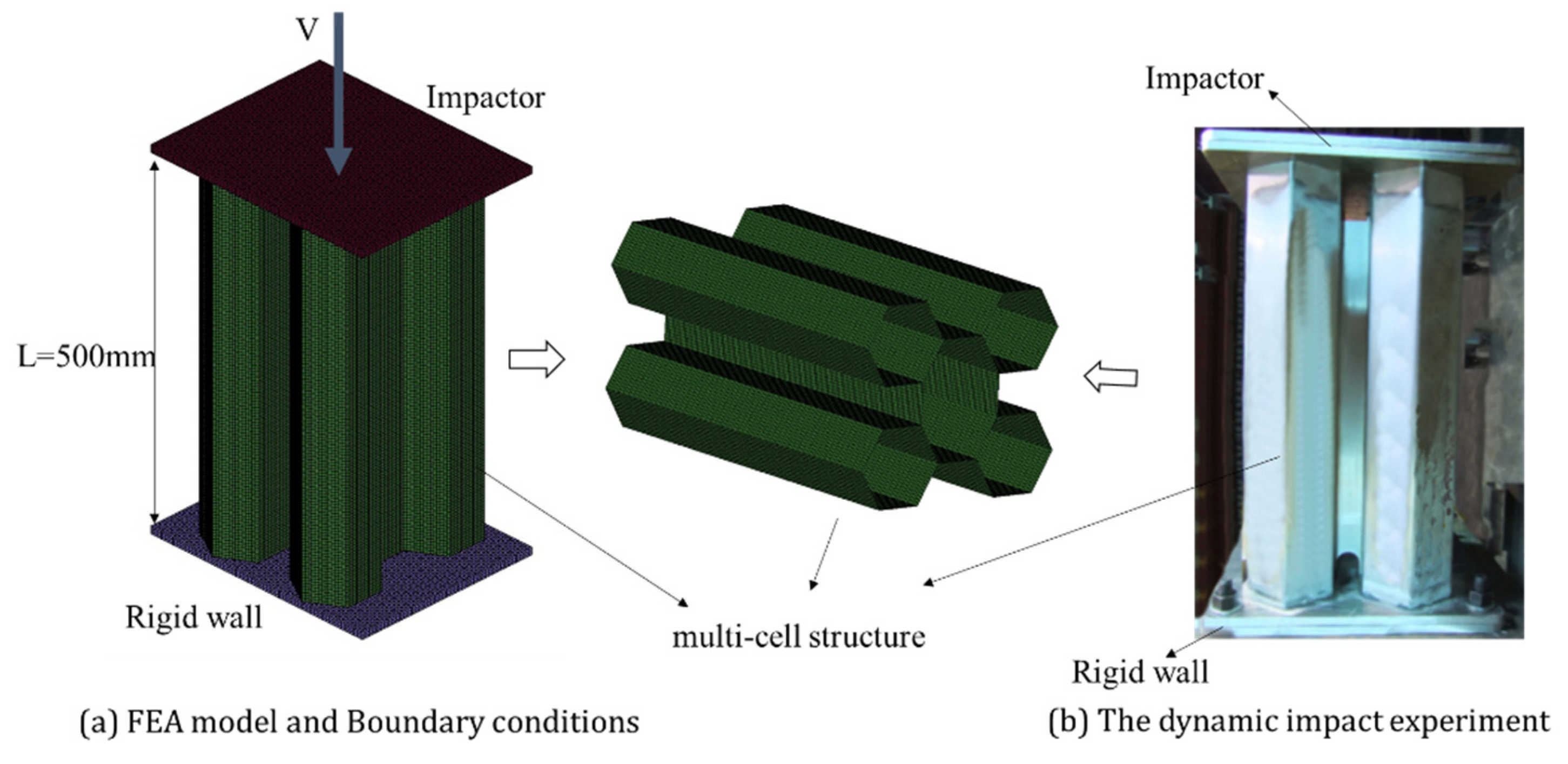
The crashworthiness performance of a multi-cell structure can be investigated using an explicit nonlinear finite element program. To simulate the deformation of energy-absorbing structures on the LS-DYNA platform, the multi-cell structure is modeled using quadrilateral shell elements of 2 × 2 mm, which are four-node shell elements with three integration points across the thickness and one integration point in the element plane. The ‘AUTOMATIC SINGLE SURFACE’ contact algorithm is used for the energy-absorbing structure’s self-contact, and the ‘AUTOMATIC SURFACE_ TO SURFACE’ contact algorithms are used to contact the rigid wall with the energy-absorbing structure, as well as the impactor with the energy-absorbing structure. There is a static coefficient of friction of 0.3 and a dynamic coefficient of friction of 0.1. During the impact, the impactor with an initial velocity of 10 m/s impacted the multi-cell structure in the X axes, while the endplates were limited in the Y and Z axes, meaning they could not move dynamically. An FE model of the multi-cell structure is shown in Figure 3a.

2.1.3. Test Set-Up

Aluminum alloy 6082-T6 is the material used in the multi-cell structure [35]. The stress–strain behavior of aluminum alloy 6082-T6 was investigated by performing quasi-static tensile tests at room temperature with strain rates of 3 × 10⁻⁴ s⁻¹ using an RGM-4300 testing machine, whose specimens were cut from a portion of a multi-cell structure. According to the linear relationship between stress and strain in the elastic phase, the test is loaded at a constant rate of 1 mm/min in the elastic phase and at a constant rate of 10 mm/min in the plasticity phase, and then the stress–strain curve of the aluminum alloy 6082-T6 can be obtained, as shown in Figure 4.

The material parameters of the aluminum alloy 6082-T6 are summarized in

Table 1. Material parameters of multi-cell structure.

Property	Units	Value
Density	kg/m3	2700
Young’s modulus	MPa	71,000
Poisson’s ratio	-	0.33
Yield stress	MPa	121
Ultimate tensile strength	MPa	183
Fracture strain	%	7.71
Fracture stress	MPa	175

. Then, the multi-cell structure material of the finite element model can be defined using Mat.024 according to the material library of the LS-DYNA platform.

Furthermore, the crashworthiness performance of the multi-cell structure can be evaluated using an experimental dynamic impactor. In order to minimize sample movement, the multi-cell structure is securely attached to the rigid wall with four bolts M30, and an initial impact velocity of 10 m/s was applied to this system. Force sensors were placed on the force homogenizing plate to measure immediate impact force, and high-speed cameras recorded the process of crushing the multi-cell structure. The deformation modes, temporal history of displacement, velocity, and crushing force can all be determined from photos taken by a high-speed digital camera through a dynamic impact experiment (Figure 2b). The crashworthiness data collected during a collision can be used to evaluate a structure’s dynamic performance, such as its deformation modes, SEA, F_m, etc.

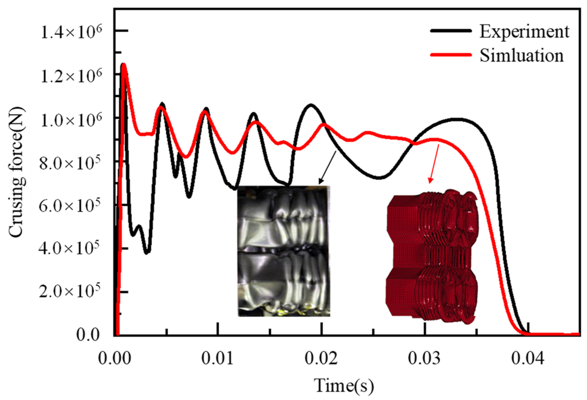
2.1.4. Crashworthiness Analysis

To assess the crashworthiness performance of the multi-cell structure, the FE simulation results were compared to dynamic impact experiment results (for the same boundary conditions), as shown in Figure 5.

Figure 5 illustrates that the simulated and test results curves are closely related, and the results from simulation and tests of the multi-cell structure have a good agreement regarding the deformation mode. In the aftermath of a collision, the crushing force reaches a peak, then declines rapidly before fluctuating. The mean crushing force continues for some time, until eventually it breaks the collapse.

Table 2. Comparison of experimental results, FE simulation results, and theoretical results.

Methods	Fm (kN)	Displacement (mm)	EA (KJ)	SEA (KJ/kg)
Experimental	874.0	278	243.0	26.9
Simulation	905.7	269	243.6	25.75
Theorical	903.3	279	252.0	26.6
Simulation Error (%)	3.6	3.2	0.2	4.2
Theorical Error (%)	3.4	3.5	3.3	3.1

provides the overall comparison of the experimental results, the simulation results, and the theoretical results.

In Table 2, F_m is 874.0 kN for test results, 905.7 kN for FE simulations, and 903.3 kN for theoretical calculations, with the errors of simulation and theoretical calculations being 3.6% and 3.4%, respectively. There is a 278 mm displacement of test results, 269 mm displacement of FE simulation results and a 279 mm displacement of theoretical results, as well as a simulation error of 3.2% and a theatrical error of 3.5%, respectively. The energy absorption (EA) of test results, FE simulation results and theoretical results are 243.0, 243.6, and 252.0 kJ, respectively, and the simulation error and theatrical error are 0.2% and 3.3%, respectively. Based on the experimental results, FE simulation results, and theoretical results, the SEA is 26.9, 25.75, and 26.66, respectively, while the simulation error and theatrical error are 4.2% and 3.1, respectively. Thus, the maximum errors in simulation results and theoretical results are no more than 4.2% and 3.5%, respectively. Besides, the comparison table showed that theoretical results and simulation results closely matched experimental results, proving that the theoretical and simulation formulas for evaluating crashworthiness are accurate.

2.2. Few-Shot Learning

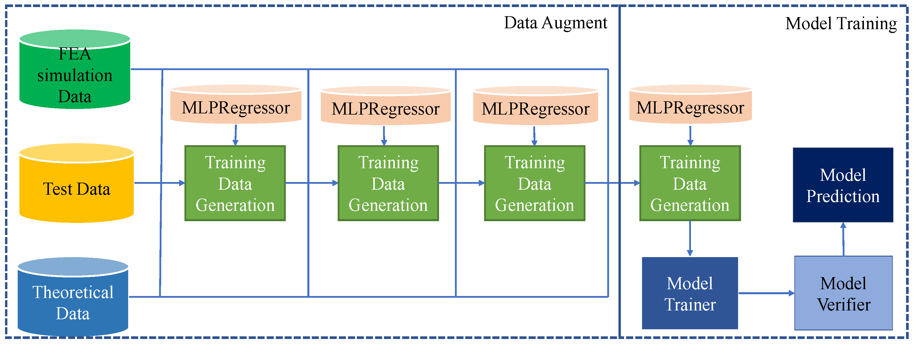
2.2.1. Data Augmentation

In crashworthiness analysis, tests and FE simulation, calculations are expensive and time-consuming, making it challenging to collect enough data; then, fewer data samples could be analyzed. The MLPRegressor is used in this paper to investigate the relationship between structural parameters and crashworthiness characteristics in order to address the limitations in sample size in engineering; then, the output of the MLPRegressor could be calculated in Equation (14).

$$y=a_k=g\left(h_k\right)=g\left({{\displaystyle \sum }}_{i=0}^M{w}_{ik}{x}_{ik}\right),$$

(14)

where y is the output of MLPRegressor, which is the final result; h_k is the input weighted sum of neurons k in the output layer. The sum-of-squares error function is:

$$E=\frac{1}{2}{{\displaystyle \sum }}_{k=1}^N{(y-y_t)}^2,$$

(15)

where y_t is the target value for the output of the network.

As seen in Figure 6, an MLPRegressor that incorporates both theoretical and FE simulation results, as well as experimental results, is proposed to ensure that this approach is correct. As a specific example of data augmentation, here are the steps:

(i) We conducted a dynamic impact experiment on multi-cell structures in the first step. FEA and theoretical results were then validated against experimental results under similar conditions.

(ii) A series of 40 FEA simulations were conducted for t = 3.5, 4.0, 4.5, 5.0 mm, and a = 45, 50, 55, 60 mm, respectively. Thus, we collected 41 samples for initial training data for MLPRegressor, which included the 40 FEA simulation and an experiment;

(iii) The three variables t ∈ [3, 6], a ∈ [20, 70], and b ∈ [14, 88] yield 4800 different combinations, which can be randomly divided into four groups, each of which has a total of 1200 combinations.

(iv) The MLPRegressor is fed with more than 1200 combinations of the first group, its output is obtained, and its validity is verified by comparing it to the theoretical results.

(v) After that, a new MLPRegressor is trained using a set of new training data, which includes an experimental sample, 40 FEA simulation samples, 1200 theoretical samples, and 1200 initial MLPRegressor samples, totaling 2441 samples.

(vi) Similar to (iv), the second dataset of 1200 combinations is fed into the latest MLPRegressor, and the output results are compared with theoretical results to ensure validity.

(vii) It is recommended that steps (v) and (vi) be repeated until all combinations of four groups have been trained and that 96041 valid sample data have been obtained.

Furthermore, not only can we obtain high-precision and representative data, but we can also increase the sample size by using a four-time hybrid technique, which gives us the foundation for training deep learning algorithm of wide and deep neural network models.

Due to the neural network’s sensitivity to input, we have to normalize the sample data after dealing with the issue of insufficient data. Specifically, in this case, we apply the MAX–MIN scaling approach in order to normalize the data according to Equation (16).

$$f\left(x_i\right)=\frac{x_i-\min \left(x\right)}{\max \left(x\right)-\min \left(x\right)},$$

(16)

In this equation, min(x) is the minimum, and max(x) is the maximum value in x.

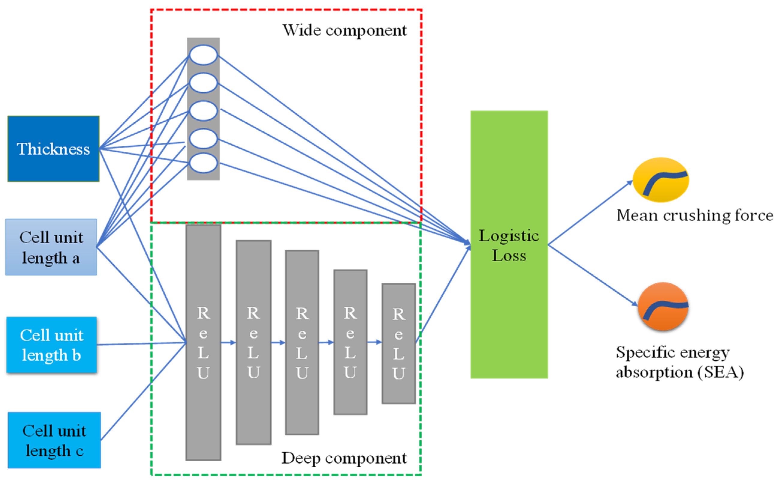
2.2.2. Model Framework

The deep learning framework of the wide and deep neural network model [36] is composed of three main components: the wide component, the deep component, and the joint training component.

• Wide component

In Figure 7, the wide component (which is contained in the red dashed box) is a layer of neural networks that are fully connected and that derives global knowledge from data. Due to this, we selected the wide component based on the multi-cell structure data (i.e., thickness and length of the cell wall) to study the co-occurrence of characteristics. Each neuron in the fully connected layer calculates its score by incorporating the multi-cell structure data into Equation (17).

$$y_j:={{\displaystyle \sum }}_{i=1}^n{w}_{i,j}{x}_i+b_1,$$

(17)

where y_j is the output of the fully connected layer in the jth neuron, n is the length of input data (x), w_i,j stands for the neuron weight between the ith input value and jth neuron, and b₁ is the bias.

The activation function of this unit will convey this number to the higher-layer connected units in order to evaluate to what extent it contributes to the prediction of the next step. The activation function is given by Equation (18).

$$u_j:=f\left(y_j\right)=\max \left(0,y_j\right),$$

(18)

where u_j is the output after activation calculation; f(·) represents the activation function.

In this study, we use a rectified linear unit as the activation function, which will only activate the positive value.

2.

Deep component

As seen in Figure 7, the deep component consists of a feed-forward neural network (enclosed in the green dash box). The multi-cell structural characteristics (thickness, cell wall lengths, etc.) are used as inputs to the model, and these low-dimensional vectors are fed into the hidden layers of the neural network through the forward pass. Specifically, each hidden layer conducts the following calculations according to Equation (19).

$$a^{\left(l+1\right)}=f\left(W^{\left(l\right)}{a}^{\left(l\right)}+b^{\left(l\right)}\right),$$

(19)

where l is the layer number; f is the activation function, generally rectified linear units (ReLUs); a^(l), b^(l), and W^(l) are the activations, bias, and model weights at the l-th layer, respectively.

3.

Joint training

Using the weighted sum of a wide component’s outputs and a deep component’s outputs, we combine the two predictions into one and use that to input a single common logistic loss function on a joint training dataset. Ensembles of models are trained independently from one another, and predictions are integrated once they have been trained. Joint training, on the other hand, optimizes all variables simultaneously, taking into account both the wide and deep components of each parameter, as well as the weights associated with their combined effect during the training process. Typically, due to the discontinuous nature of training, it is necessary that each model be larger (e.g., have more features and transformations) for the ensemble to perform correctly. In contrast, during joint training, the wide part requires just a modest number of cross-product feature transformations to compensate for the deep part’s shortcomings, rather than a full-size wide model.

Using mini-batch stochastic optimization, the wide component and deep component of the deep learning model are trained simultaneously using the gradients from the output. In the test, we used RMSprop as the optimizer for the wide component of the model, and AdaGrad for the deep component. In Figure 7, the combined model is illustrated, and a logistic regression model’s prediction is given by Equation (20).

$$P\left(Y=1\mid x\right)=\sigma \left(w_{wide}^T\left[x,\varphi \left(x\right)\right]+w_{\mathrm{deep}}^T{a}^{\left(l_f\right)}+b\right),$$

(20)

where Y is the binary class label; σ(·) is the sigmoid function; φ(x) is the cross-product transformations of the original features x; b is the bias term; w_wide is the vector of all wide components weights; w_deep are the weights applied on the final activations a^(lf).

The pseudo code used for the few-shot learning combined with data augmentation and wide and deep neural networks is shown in Algorithm 1.

Algorithm 1. Few-shot learning pseudo code.

Few-Shot Learning in This Study

hybrid data augmentation to obtain dataset

initialize all variables by the random value

for loop from 1 to num_epoch

choose xi from X data as the wide model input

choose xj from X data as the deep model input

compute the yj of the wide model output

$\hspace{1em}\hspace{1em}\hspace{1em}\hspace{1em}\hspace{1em}\hspace{1em}\hspace{1em}\hspace{1em}\hspace{1em}{y}_j:={\displaystyle \sum }_{i=1}^n{\mathit{w}}_{i,j}{x}_i+b_1$

compute the output of the deep model output-layer a(l+1)

for l = L to 5:

compute the a(l + 1) based on a(l) and W(l) and b(l)

$\hspace{1em}\hspace{1em}\hspace{1em}\hspace{1em}\hspace{1em}\hspace{1em}\hspace{1em}\hspace{1em}\hspace{1em}\hspace{1em}\hspace{1em}\hspace{1em}{a}^{\left(l+1\right)}=f\left(W^{\left(l\right)}{a}^{\left(l\right)}+b^{\left(l\right)}\right)$

concatenate the wide output and deep output, and compute the model output

$\hspace{1em}\hspace{1em}\hspace{1em}\hspace{1em}\hspace{1em}\hspace{1em}\hspace{1em}\hspace{1em}\left(Y=1\mid x\right)=\sigma \left(w_{wide}^T\left[x,\varphi \left(x\right)\right]+w_{\mathrm{deep}}^T{a}^{\left(l_f\right)}+b\right)$

2.3. Problem Set-Up

2.3.1. Optimization Problem

Multi-cell structures are characteristic of high-speed trains that absorb a great deal of energy during a collision. These energy-absorbing structures must prevent uncontrolled collapse and protect the occupied volume from being damaged during the collapse process, as well as ensure the proper functioning of the energy-absorbing components at each end of the train. Multi-cell structures, as important energy-absorbing components, should be optimized to obtain higher energy-absorbing efficiency and lighter mass. To achieve crashworthiness standards, a powerful optimization tool is introduced into the design of multi-cell energy-absorbing structures. There would be an improvement in the crashworthiness of the energy-absorbing structures on the high-speed train if the multi-cell energy-absorbing structure had a higher F_m and SEA. Meanwhile, multi-cell structures have the advantage of absorbing more energy while being lighter in mass, which provides high efficiency of energy absorption, thereby increasing the crashworthiness of energy-absorbing components.

Our goal is to minimize crash damage loss by optimizing the maximum F_m, maximum SEA, and minimum mass (M) of the multi-cell structure. A multi-objective optimization model of multi-cell structures, with the main objective of maximizing F_m, SEA and minimizing M, can be analyzed in this study. Furthermore, the geometry of the high-speed train’s front end constrains the cross-sectional area of the energy absorption structure, the scale of the total energy absorption is also constrained as a result of the tight design space, and then the amount of the design space is used as a constraint in the optimization problem. Following that, the optimization function is described with respect to the design variables of t, a, b, and c. In summary, the multi-objective optimization problem can be expressed as Equation (21).

$$\{\begin{array}{l}\mathrm{Max}\left[F_m\left(t,a,b,c\right),S_{EA}\left(t,a,b,c\right),1/\mathrm{M}\left(t,a,b,c\right)\right]\hfill \\ \mathrm{s}.\mathrm{t}.3 \mathrm{mm}\le t\le 6 \mathrm{mm}\hfill \\ 40 \mathrm{mm}\le a\le 70 \mathrm{mm}\hfill \\ 0 \mathrm{mm}\le b\le 122 \mathrm{mm}\hfill \\ 0 \mathrm{mm}\le c\le 123 \mathrm{mm}\hfill \\ \max \left(4\left(a+t\right)+c,2\sqrt{3}\left(a+t\right)+b\right)\le 300 \mathrm{mm}\hfill \\ \min \left(4\left(a+t\right)+c,2\sqrt{3}\left(a+t\right)+b\right)\le 265 \mathrm{mm}\hfill \end{array},$$

(21)

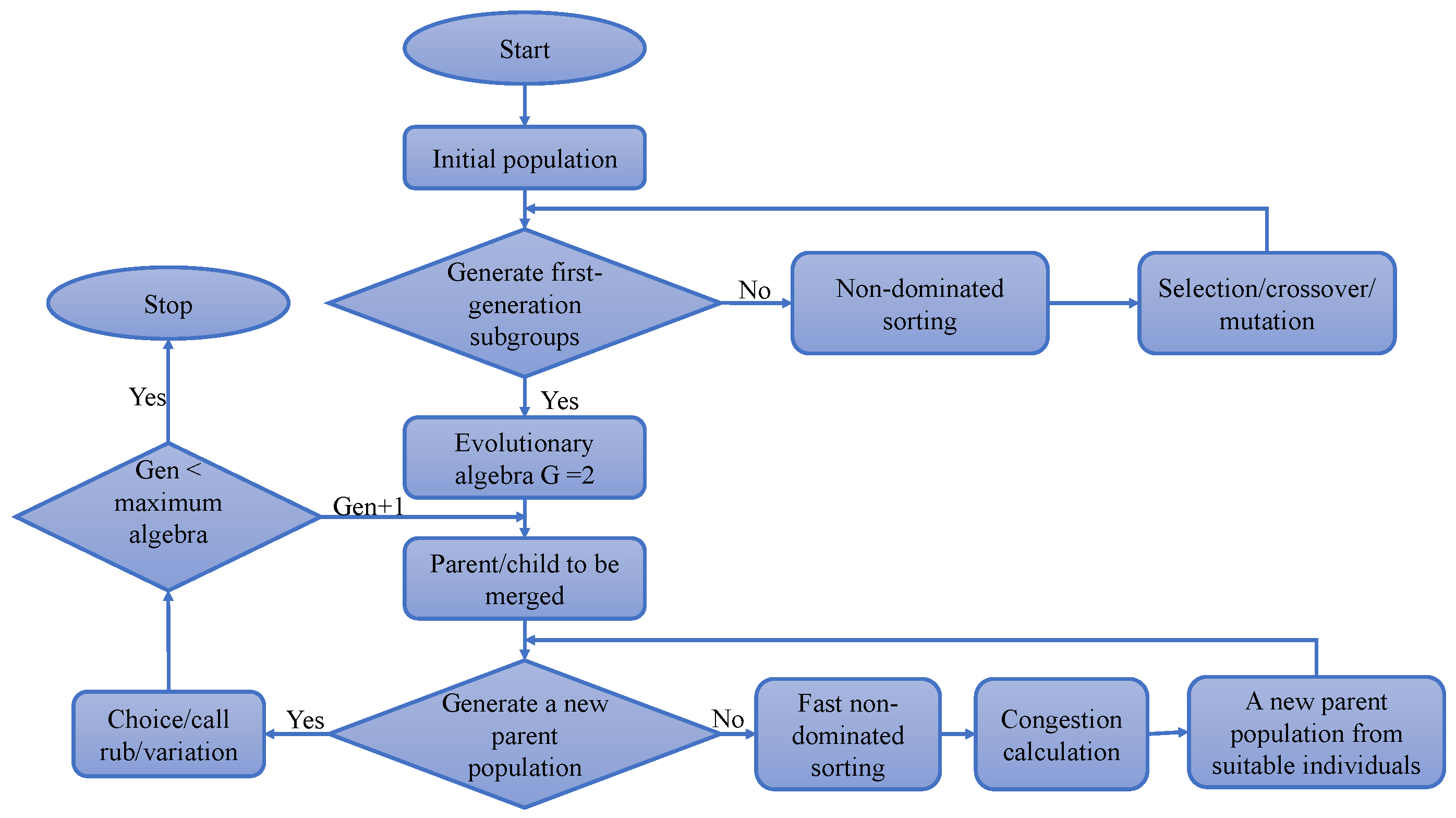
2.3.2. Optimization Algorithm

Non-dominated Sorting Genetic Algorithm-III (NSGA-III) is an adaptation of a genetic algorithm for solving problems involving multi-objective optimization [37]. Multi-objective optimization is concerned with the minimization or maximization of more than one objective function simultaneously, and the objective is not just to determine an optimum but also to identify the Pareto front. Figure 8 shows a flow chart of the multi-objective optimization process.

3. Results and Discussion

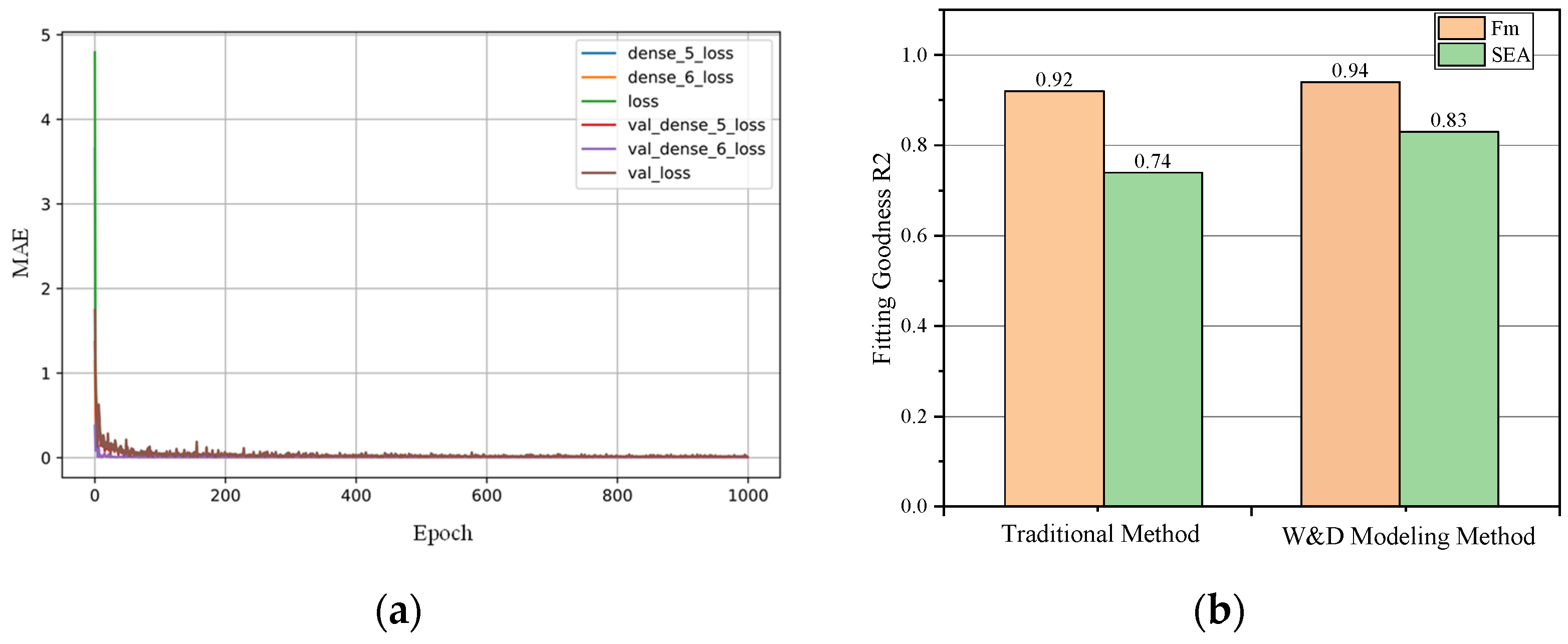
3.1. Model Training

By applying wide and deep neural networks to the few-shot learning approach, we evaluate every structural parameter, such as wall thickness t, cell length a, cell length b, and cell length c in the deep component, and thickness and unit wall length in the broad component. To achieve the best performance, k-fold cross-validation, which divides the training data and verification data by 0.75 and 0.25, resulting in 7231 tests for training and 2410 for validation. Then, the hyperparameters (hidden layers = 5, layer size 1 = 1024, layer size 2 = 512, layer size 3 = 256, layer size 4 = 128 and layer size 5 = 64, optimizer = RMSprop, learning rate = 0.0001) are defined through a coarse grid search. Concatenating these dense features results in a dense vector of approximately 19285 dimensions. Afterward, the concatenated vector is fed into five ReLU layers and then into the logistic output unit, from which dense and sparse features are generated during training.

As a result of 1000 training sessions, the mean absolute error (MAE) of the loss, representing the value of the training set’s loss, and the val_loss, representing the value of the test set’s loss, both remain essentially stable, as shown in Figure 9a. In addition, in order to further validate the accuracy of the prediction, both the few-shot learning and the Radial Basis Function (RBF) models [38] are evaluated by examining its goodness-of-fit R2 (the closer the value is to 1, the better the fitting), and the results are shown in Figure 9b.

Figure 9 clearly indicates that both the few-shot learning model and the RBF model are well-trained. The few-shot learning model of F_m and SEA has a goodness-of-fit of 0.94 and 0.8, respectively, while the traditional RBF model has a goodness-of-fit of 0.92 and 0.74, namely, the few-shot learning model’s goodness-of-fit is higher than the traditional RBF model’s. Additionally, to estimate the mean force and SEA of this approach, the response surface comparison results and the contour line comparison results of the mean force and SEA are derived from the traditional RBF model and the few-shot learning model, as shown in Figure 10.

As shown in Figure 10, the fluctuation of four critical factors can be accurately assessed by comparing the response surface and contours of the RBF model and the few-shot learning model. For the combination of parameters t = 7.1 mm, a = 81 mm, b = 98 mm, and c = 82 mm, the maximum force calculated by the few-shot learning model is 2013.75 kN, while the maximum force calculated by the traditional RBF met hod is 1858.84 kN, producing an error of 7.6%. With parameters t = 7.1 mm, a = 11 mm, b = 4 mm, and c = 2.5 mm, the few-shot learning model calculates a maximum SEA of 81.233, whereas the traditional RBF model calculates a maximum SEA of 83.616, which yields a 2.7% error. Comparison results show that the errors are all within the acceptable range and that the few-shot learning model can accurately predict the outcome in terms of accuracy. Finally, we obtain the response results from twelve arrays generated randomly based on the data points, and they are used to test the validity of the few-shot learning model. In

Table 3. Comparison response results.

Test	t (mm)	a (mm)	b (mm)	c (mm)	Fm (kN)			SEA
					Actual	Predicted	Eror	Actual	Predicted	Error
1	4.2	57	67	44	761.11	749.03	0.015	26.078	28.034	−0.07
2	5.7	69	41	46	1116.38	1114.536	0.002	28.729	31.34	−0.09
3	4.7	70	67	68	931.48	952.34	−0.025	29.2	32.456	−0.111
4	5.7	47	48	69	1006.12	1007.639	−0.001	33.272	36.299	−0.09
5	3.6	61	69	63	629.65	651.34	−0.034	23.16	28.67	−0.237
6	5.9	69	63	64	1231.12	1218.28	0.01	32.29	34.85	−0.08
7	5.4	69	98	67	1140.87	1134.53	0.006	35.88	36.5	−0.017
8	3.6	70	67	68	668.87	700.87	−0.047	21.8	28.82	−0.322
9	4.2	42	58	48	666.69	668.17	−0.002	29.77	29.16	0.02
10	3.8	79	31	63	749.89	776.08	−0.03	21.67	28.35	−0.30
11	4.3	47	68	70.5	741.17	756.45	−0.02	28.07	32.37	−0.15
12	1.33	11	4	82	71.022	131.23	−0.84	28.02	30.23	−0.07

, we summarize the response results for various control parameter combinations.

As shown in Table 3, the largest difference in F_m between the actual and the few-shot learning model predicted is 0.84, and the largest difference in SEA between the actual and the few-shot learning model predicted is 0.322. Overall, the few-shot learning model is more accurate and performs better in terms of generalization. After this introduction, it is possible to conduct a parametric study and an optimization analysis based on the surrogate model in the following sections.

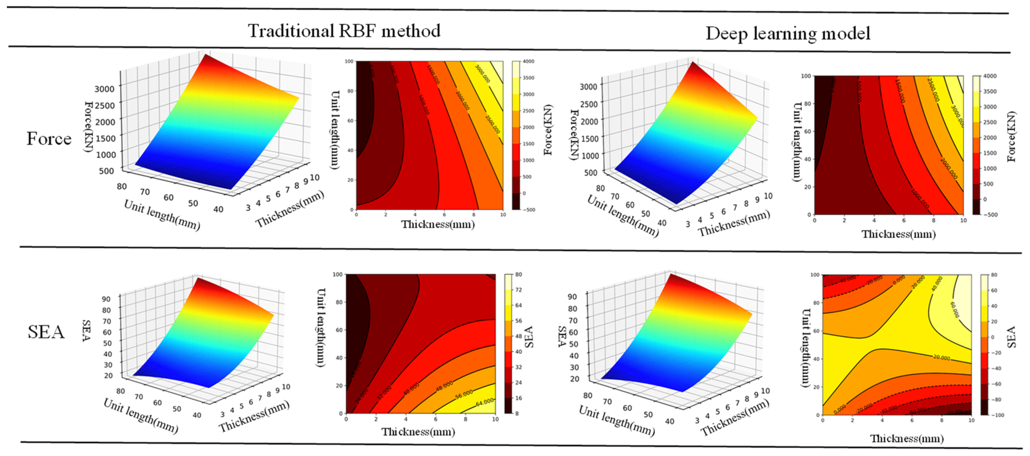
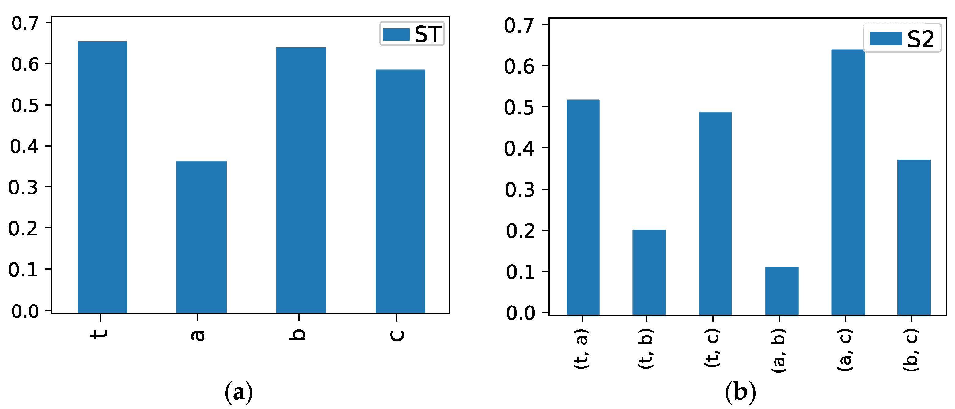
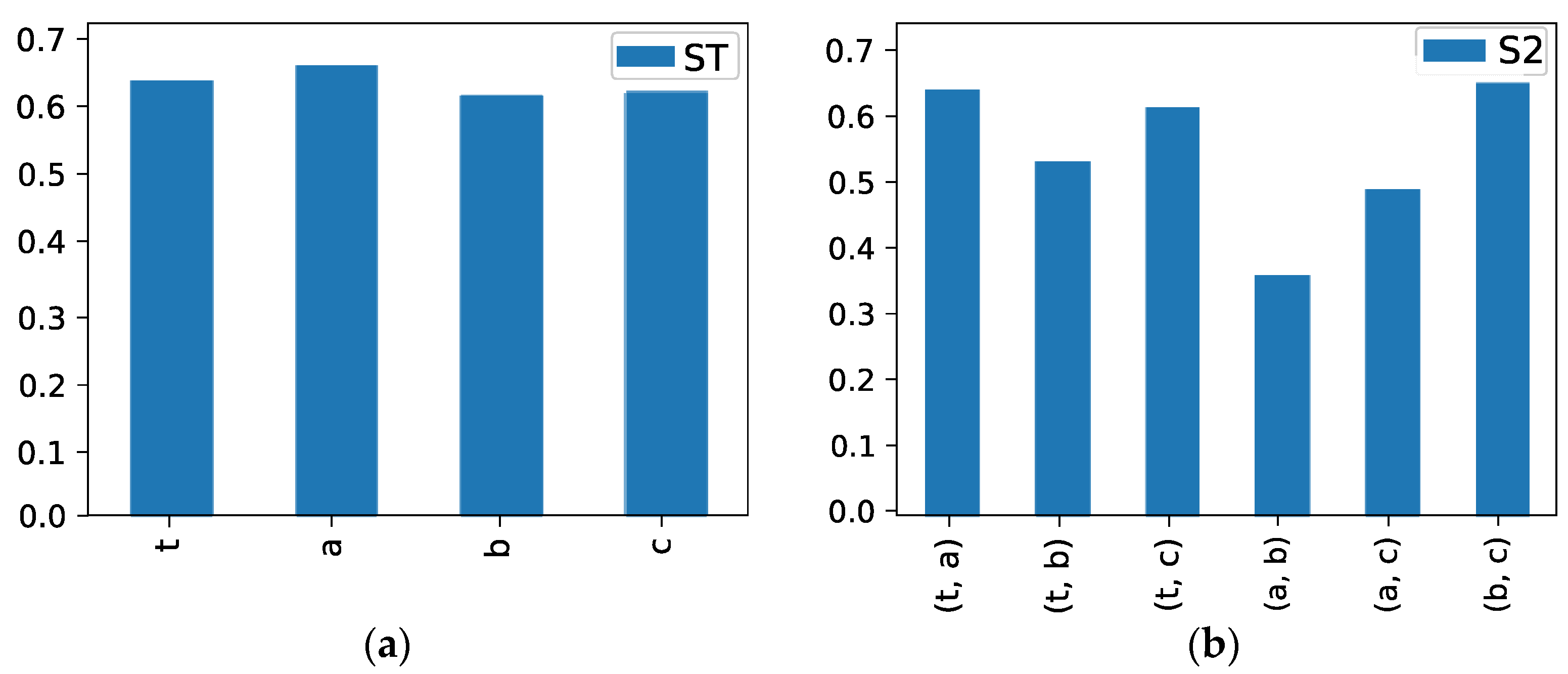
3.2. Parametric Study

According to [39], the structure parameters can influence crashworthiness, so it is important to investigate the parametric sensitivity analysis of crashworthiness. For a deeper understanding of the influence of each parameter on the F_m, the total sensitivity indices (ST) at 95% confidence levels considered the mutual influence, and the second-order sensitivity indices (S2) at 95% confidence levels also include the mutual influence, as shown in Figure 11.

According to Figure 11, the cell wall length b is the most important structural factor affecting mean crushing force, followed by the thickness t, and cell wall length a is the least crucial factor. The most significant effect on the mean force is the interaction between cell wall length a and cell wall length c, followed by the interaction between the thickness t and the cell wall length c. The interaction between cell wall length a and cell wall length b of the cell wall has the least effect. Additionally, to analyze the influence of each parameter on SEA, we calculate the total sensitivity indices (ST) at a 95% confidence level, including the influences between each parameter, and we also calculate the second-order sensitivity indices (S2) at a 95% confidence level incorporating the mutual influence, as shown in Figure 12.

Figure 12 shows that thickness t and cell wall length a had the greatest impact on the SEA of all structural factors, followed by cell wall length b and cell wall length c. The interaction between thickness t and cell wall length a, and also the interaction between cell wall length b and cell wall length c, has the greatest influence on SEA. The interaction between thickness t and cell wall length c has the next greatest effect on SEA, while the interaction between cell wall length a and cell wall length b has the least influence on SEA. Considering all the structural parameters, the parametric analysis shows that both thickness t, cell wall lengths a, b, and c, and their interactions have a significant impact on F_m and SEA and, consequently, provide a basis for further optimization of the multi-cell structure’s crashworthiness index.

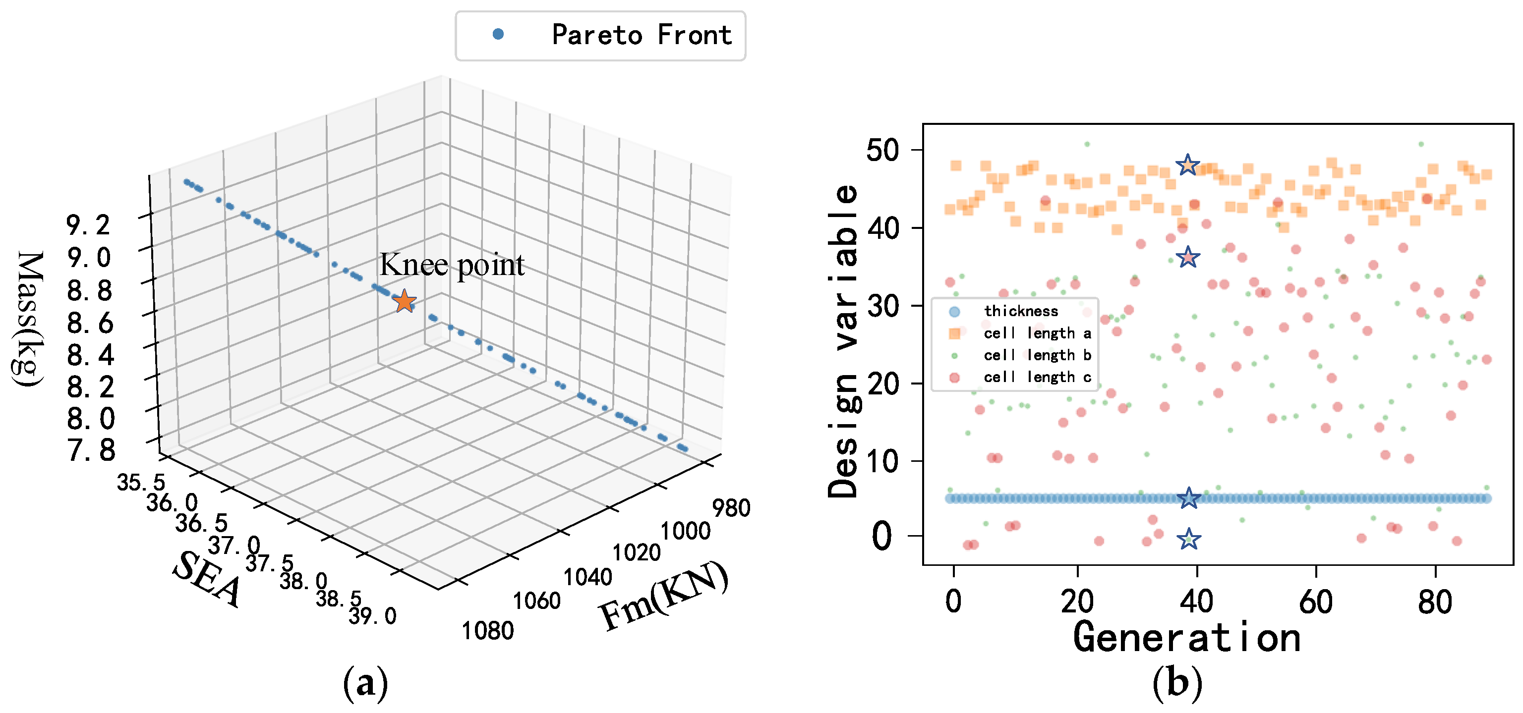
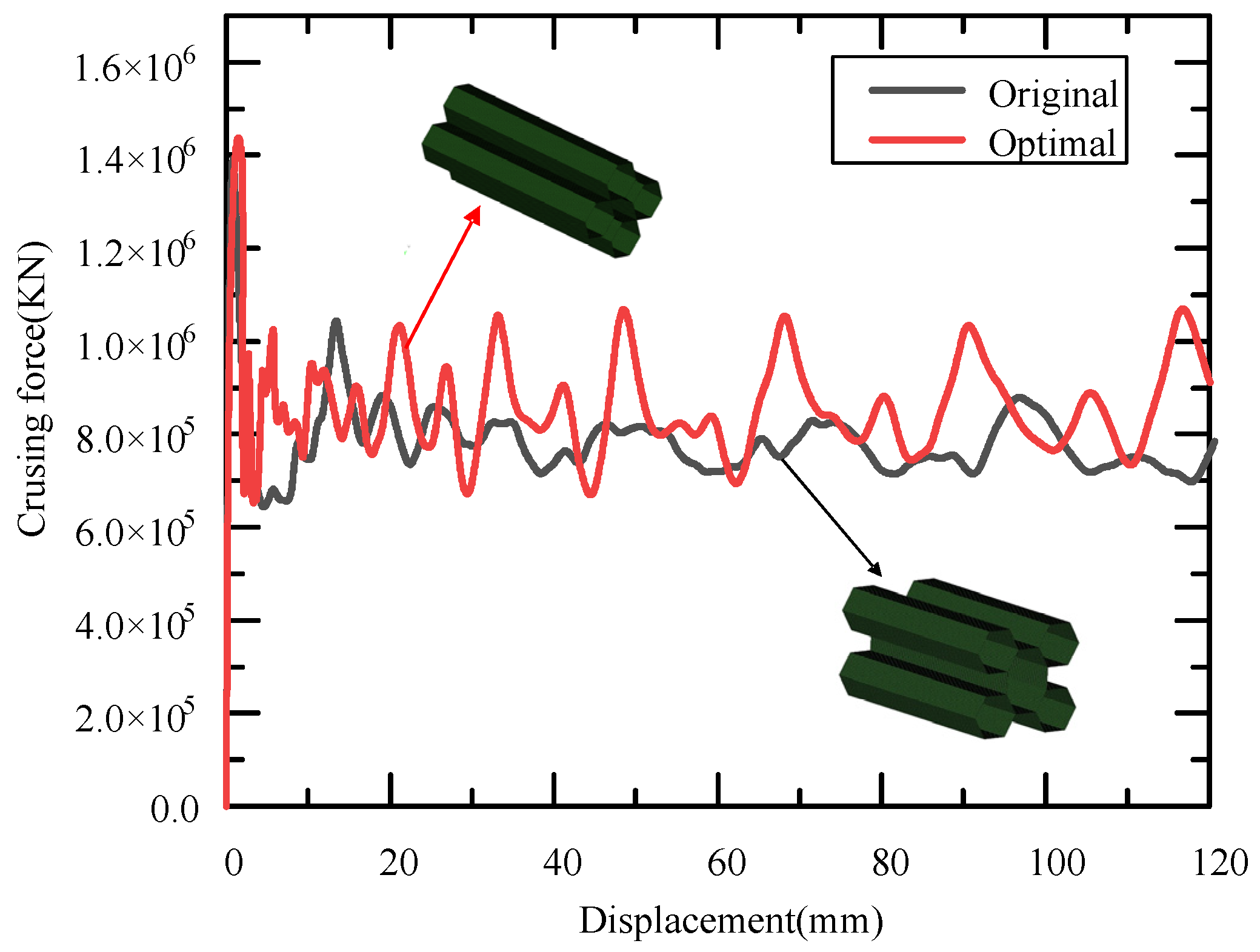
3.3. Optimisation Results

A specified description of the parameter definitions for the NSGA-III algorithm may be given: the population size, maximum iteration, generation gap, crossover rate, and mutation rate are 1000, 500, 0.8, 0.9, and 0.1, respectively. The NSGA-III algorithm generates a well-distributed Pareto front throughout the design space, and Figure 13 shows the Pareto front generated from the optimization function in this study, with the “star” indicating the parameters that were selected as optimal.

The optimal parameters of the t, a, b, and c are calculated, and the results show that the t is approximately 6 mm, the a is approximately 50 mm, and the b and c are relatively flexible. In terms of an integrative argument, t, a, b, and c are 5.99, 48.68, 0.71, and 36.86 mm respectively, so we could take the integer parameters to mean that t, a, b, and c are 6, 49, 0, and 37 mm, respectively. The optimal results and original results are modeled on the platform of LS-DYNA based on an impact speed of 10m/s in order to validate the effectiveness of the optimization algorithm and to evaluate the crashworthiness performance of the multi-cell energy-absorbing structure. Figure 14 shows the force–displacement curves associated with the optimal design and the initial design.

Table 4. Comparison of the optimum design and the initial design.

Design	t (mm)	a (mm)	b (mm)	c (mm)	Fm (kN)	EA (kJ)	SEA (kJ/kg)	M (kg)
Initial	5	56	56	51	905.7	243.6	25.75	9.46
Optimal	6	49	0	37	1060.9	333.9	36.86	9.06
Change	0.20	−0.125	-	−0.274	0.171	0.371	0.301	−0.040

details the critical indexes of these two designs.

The dynamic force curve of an optimum design is more constant with a greater maximum force, as shown in Figure 14. According to Figure 14, in the event of an impact, dynamic crushing force peaks initially, then drops rapidly, and oscillates around the average crushing force, eventually completing telescopic deformation. Furthermore, the optimized multi-cellular structure displays a higher average crushing force than the original design, meaning that when it compresses the same distance, it absorbs a greater amount of energy. Consequently, the energy-absorbing structures of the high-speed train are improved in terms of its crashworthiness.

As depicted in Table 4, compared with the original design, the crashworthiness index of the optimal design has also been improved, and the SEA and F_m are increased by 30.1% and 17.1%, respectively, for the requirements of the Energy Absorption (EA). Meanwhile, the structural mass of the optimized design is also reduced by 4% at the same time. Therefore, the optimized structure is significant with great potential in crashworthiness applications for multi-cell structures of high-speed trains.

4. Conclusions

In an effort to analyze and optimize the crashworthiness of multi-cell structures with hexagonal cells, a deep learning-based few-shot learning model has been developed, and its applications on multi-objective optimisation illustrate its significant potential.

In this study, we attempt to solve the problem of insufficient data in engineering via a few-shot learning approach based on the hybrid augmentation technique that uses SSFE theory and FE simulations to supplement existing data. A multi-cell structure of high-speed trains under axial dynamic impact load is analyzed using a wide and deep neural network model to explore the crashworthiness characteristics, especially F_m and SEA. This deep learning could provide the memory capacity of the shallow network and the generalization ability of the deep model. The deep learning model of wide and deep neural networks has excellent results and is in agreement with actual results. Therefore, this deep learning-based few-shot learning model provides a thorough and accurate description of the dynamic behavior of collisions.

To develop design guidelines for multi-cell structures, parametric sensitivity analysis is applied to determine the effects of design variables on collision responses, and multiobject optimization is applied to multi-cell structures. Using the NSGA-III algorithm, the multi-cell structure’s crashworthiness characteristics of F_m, SEA, and M are then optimized. By adjusting the wall thickness and the cell side length, the optimal structure of the F_m, SEA, and M achieved 1060.9 kN, 36.86 kJ/kg, and 9.06 kg, respectively, which effectively improved the load-bearing capacity of the multi-cell structure.

Still, there is room for improvement here in the future. (i) There may be opportunities to enhance the extrapolation capability of this proposed approach in the future. (ii) Considering that there are a variety of different approaches that can be utilized for this application, it would be of interest to investigate the performance of another algorithm in the future. (iii) Multi-cell structures should be pre-crushed to reduce the static/dynamic ratio and to make them more uniform, and it is recommended that the dynamic crush coefficient should consider additional factors, such as the material, shape, and size, in order to achieve greater accuracy. (iv) Optimization of the multi-cell structure under more complex crash conditions should be investigated and implemented in the future. Furthermore, we believe that this study may be useful for optimizing other safety functions in the future.

References

1. Chou, S.; Rhodes, J. Review and compilation of experimental results on thin-walled structures. Comput. Struct. 1997, 65, 47–67. [Google Scholar] [CrossRef]
2. Bull, J.W. Finite Element Analysis of Thin-Walled Structures; CRC Press: London, UK, 1988. [Google Scholar]
3. Bischoff, M.; Ramm, E.; Irslinger, J. Models and finite elements for thin-walled structures. In Encyclopedia of Computational Mechanics, 2nd ed.; John Wiley & Sons, Ltd.: Chichester, UK, 2004; Volume 2, pp. 1–86. [Google Scholar]
4. Chen, W.; Wierzbicki, T. Relative merits of single-cell, multi-cell and foam-filled thin-walled structures in energy absorption. Thin-Walled Struct. 2001, 39, 287–306. [Google Scholar] [CrossRef]
5. Susac, F.; Beznea, E.F.; Baroiu, N. Artificial Neural Network Applied to Prediction of Buckling Behaviour of the Thin Walled Box. Advanced Engineering Forum; Trans Tech Publications: Zurich, Switzerland, 2017; Volume 21, pp. 141–150. [Google Scholar]
6. Tang, Z.; Zhu, Y.; Nie, Y.; Guo, S.; Liu, F.; Chang, J.; Zhang, J. Data-driven train set crash dynamics simulation. Veh. Syst. Dyn. 2017, 55, 149–167. [Google Scholar] [CrossRef]
7. Dong, S.; Tang, Z.; Yang, X.; Wu, M.; Zhang, J.; Zhu, T.; Xiao, S. Nonlinear Spring-Mass-Damper Modeling and Parameter Estimation of Train Frontal Crash Using CLGAN Model. Shock Vib. 2020, 2020, 9536915. [Google Scholar] [CrossRef]
8. Acar, E. Increasing automobile crash response metamodel accuracy through adjusted cross validation error based on outlier analysis. Int. J. Crashworthiness 2015, 20, 107–122. [Google Scholar] [CrossRef]
9. Wei, Z.; Robbersmyr, K.G.; Karimi, H.R. Data-based modeling and estimation of vehicle crash processes in frontal fixed-barrier crashes. J. Frankl. Inst. 2017, 354, 4896–4912. [Google Scholar] [CrossRef]
10. Karimi, H.R.; Pawlus, W.; Robbersmyr, K.G. Signal reconstruction, modeling and simulation of a vehicle full-scale crash test based on morlet wavelets. Neurocomputing 2012, 93, 88–99. [Google Scholar] [CrossRef]
11. Wang, Y.; Yao, Q.; Kwok, J.T.; Ni, L.M. Generalizing from a few examples: A survey on few-shot learning. ACM Comput. Surv. 2020, 53, 1–34. [Google Scholar] [CrossRef]
12. Argüeso, D.; Picon, A.; Irusta, U.; Medela, A.; San-Emeterio, M.G.; Bereciartua, A.; Alvarez-Gila, A. Few-Shot Learning approach for plant disease classification using images taken in the field. Comput. Electron. Agric. 2020, 175, 105542. [Google Scholar] [CrossRef]
13. Ren, Z.; Zhu, Y.; Yan, K.; Chen, K.; Kang, W.; Yue, Y.; Gao, D. A novel model with the ability of few-shot learning and quick updating for intelligent fault diagnosis. Mech. Syst. Signal Process. 2020, 138, 106608. [Google Scholar] [CrossRef]
14. Sun, X.; Wang, B.; Wang, Z.; Li, H.; Li, H.; Fu, K. Research progress on few-shot learning for remote sensing image interpretation. IEEE J. Sel. Top. Appl. Earth Obs. Remote Sens. 2021, 14, 2387–2402. [Google Scholar] [CrossRef]
15. Nia, A.A.; Parsapour, M. Comparative analysis of energy absorption capacity of simple and multi-cell thin-walled tubes with triangular, square, hexagonal and octagonal sections. Thin-Walled Struct. 2014, 74, 155–165. [Google Scholar]
16. Guler, M.A.; Cerit, M.E.; Bayram, B.; Gerceker, B.; Karakaya, E. The effect of geometrical parameters on the energy absorption characteristics of thin-walled structures under axial impact loading. Int. J. Crashworthiness 2010, 15, 377–390. [Google Scholar] [CrossRef]
17. Guillow, S.; Lu, G.; Grzebieta, R. Quasi-static axial compression of thin-walled circular aluminium tubes. Int. J. Mech. Sci. 2001, 43, 2103–2123. [Google Scholar] [CrossRef]
18. Fan, Z.; Lu, G.; Liu, K. Quasi-static axial compression of thin-walled tubes with different cross-sectional shapes. Eng. Struct. 2013, 55, 80–89. [Google Scholar] [CrossRef]
19. Tai, Y.; Huang, M.; Hu, H.-T. Axial compression and energy absorption characteristics of high-strength thin-walled cylinders under impact load. Theor. Appl. Fract. Mech. 2010, 53, 1–8. [Google Scholar] [CrossRef]
20. Shim, V.-W.; Stronge, W. Lateral crushing of thin-walled tubes between cylindrical indenters. Int. J. Mech. Sci. 1986, 28, 683–707. [Google Scholar] [CrossRef]
21. Baroutaji, A.; Gilchrist, M.D.; Smyth, D.; Olabi, A.G. Crush analysis and multi-objective optimisation design for circular tube under quasi-static lateral loading. Thin-Walled Struct. 2015, 86, 121–131. [Google Scholar] [CrossRef]
22. Niknejad, A.; Elahi, S.M.; Elahi, S.A.; Elahi, S.A. Theoretical and experimental study on the flattening deformation of the rectangular brazen and aluminium columns. Arch. Civ. Mech. Eng. 2013, 13, 449–464. [Google Scholar] [CrossRef]
23. Tran, T.; Baroutaji, A. Crashworthiness optimal design of multi-cell triangular tubes under axial and oblique impact loading. Eng. Fail. Anal. 2018, 93, 241–256. [Google Scholar] [CrossRef]
24. Ying, L.; Dai, M.; Zhang, S.; Ma, H.; Hu, P. Multiobjective crashworthiness optimisation of thin-walled structures with functionally graded strength under oblique impact loading. Thin-Walled Struct. 2017, 117, 165–177. [Google Scholar] [CrossRef]
25. Alkhatib, S.E.; Tarlochan, F.; Hashem, A.; Sassi, S. Collapse behaviour of thin-walled corrugated tapered tubes under oblique impact. Thin-Walled Struct. 2018, 122, 510–528. [Google Scholar] [CrossRef]
26. Zhang, X.; Zhang, H.; Wang, Z. Bending collapse of square tubes with variable thickness. Int. J. Mech. Sci. 2016, 106, 107–116. [Google Scholar] [CrossRef]
27. Du, Z.; Duan, L.; Cheng, A.; Xu, Z.; Zhang, G. Theoretical prediction and crashworthiness optimisation of thin-walled structures with single-box multi-cell section under three-point bending loading. Int. J. Mech. Sci. 2019, 157, 703–714. [Google Scholar] [CrossRef]
28. Duan, L.; Xiao, N.C.; Li, G.; Xu, F.; Chen, T.; Cheng, A. Bending analysis and design optimisation of tailor-rolled blank thin-walled structures with top-hat sections. Int. J. Crashworthiness 2017, 22, 227–242. [Google Scholar] [CrossRef]
29. Baroutaji, A.; Sajjia, M.; Olabi, A.-G. On the crashworthiness performance of thin-walled energy absorbers: Recent advances and future developments. Thin-Walled Struct. 2017, 118, 137–163. [Google Scholar] [CrossRef]
30. Chen, T.; Zhang, Y.; Lin, J.; Lu, Y. Theoretical analysis and crashworthiness optimisation of hybrid multi-cell structures. Thin-Walled Struct. 2019, 142, 116–131. [Google Scholar] [CrossRef]
31. Chen, J.; Xu, P.; Yao, S.; Xing, J.; Hu, Z. The multi-objective structural optimisation design to improve the crashworthiness of a multi-cell structure for high-speed train. Int. J. Crashworthiness 2020, 27, 24–33. [Google Scholar] [CrossRef]
32. Langseth, M.; Hopperstad, O.S. Static and dynamic axial crushing of square thin-walled aluminium extrusions. Int. J. Impact Eng. 1996, 18, 949–968. [Google Scholar] [CrossRef]
33. Wierzbicki, T.; Abramowicz, W. On the crushing mechanics of thin-walled structures. J. Appl. Mech. 1983, 50, 727–739. [Google Scholar] [CrossRef]
34. Abramowicz, W.; Wierzbicki, T. Axial crushing of multicorner sheet metal columns. J. Appl. Mech. 1989, 56, 113–120. [Google Scholar] [CrossRef]
35. Zhao, Y.; Zhai, X.; Sun, L. Test and design method for the buckling behaviours of 6082-T6 aluminium alloy columns with box-type and L-type sections under eccentric compression. Thin-Walled Struct. 2016, 100, 62–80. [Google Scholar] [CrossRef]
36. Cheng, H.T.; Koc, L.; Harmsen, J.; Shaked, T.; Chandra, T.; Aradhye, H.; Anderson, G.; Corrado, G.; Chai, W.; Ispir, M.; et al. Wide & deep learning for recommender systems. In Proceedings of the 1st Workshop on Deep Learning for Recommender Systems, Boston, MA, USA, 15 September 2016; pp. 7–10. [Google Scholar]
37. Deb, K.; Jain, H. An Evolutionary Many-Objective Optimization Algorithm Using Reference-Point-Based Nondominated Sorting Approach, Part I: Solving Problems with Box Constraints. IEEE Trans. Evol. Comput. 2014, 18, 577–601. [Google Scholar] [CrossRef]
38. He, Q.; Shahabi, H.; Shirzadi, A.; Li, S.; Chen, W.; Wang, N.; Chai, H.; Bian, H.; Ma, J.; Chen, Y.; et al. Landslide spatial modelling using novel bivariate statistical based Naïve Bayes, RBF Classifier, and RBF Network machine learning algorithms. Sci. Total Environ. 2019, 663, 1–15. [Google Scholar] [CrossRef] [PubMed]
39. Douglas-Smith, D.; Iwanaga, T.; Croke, B.F.; Jakeman, A.J. Certain trends in uncertainty and sensitivity analysis: An overview of software tools and techniques. Environ. Model. Softw. 2020, 124, 104588. [Google Scholar] [CrossRef]
Figure 1. Multi-cell structure of the high-speed train.
Machines 10 00696 g001
Figure 2. Three-panel element and simplification: (a) V angle element and right corner element; (b) Y-I unit element; (c) V-shaped unit element.
Machines 10 00696 g002
Figure 3. FE model and impact test of multi-cell structure.
Machines 10 00696 g003
Figure 4. Plastic stress–strain behavior of the aluminum alloy 6082-T6.
Machines 10 00696 g004
Figure 5. The force–time history curves of experiment and simulation.
Machines 10 00696 g005
Figure 6. Data augmentation overview.
Machines 10 00696 g006
Figure 7. Deep learning framework.
Machines 10 00696 g007
Figure 8. Flowchart of the NSGA-III.
Machines 10 00696 g008
Figure 9. Training procedure: (a) loss curves on epochs; (b) fitting goodness R2.
Machines 10 00696 g009
Figure 10. Estimation of few-shot learning model.
Machines 10 00696 g010
Figure 11. Sensitivity analysis of Fm: (a) ST at 95% confidence level; (b) S2 at 95% confidence level.
Machines 10 00696 g011
Figure 12. Sensitivity analysis of SEA: (a) ST at 95% confidence level; (b) S2 at 95% confidence level.
Machines 10 00696 g012
Figure 13. Pareto front solution: (a) Pareto front; (b) the optimal parameters results.
Machines 10 00696 g013
Figure 14. The force–displacement curves of two designs.
Machines 10 00696 g014