
Evaluation of Rolling Bearing Performance Degradation Based on Comprehensive Index Reduction and SVDD


Abstract
:1. Introduction
2. Feature Extraction and Dimensionality Reduction
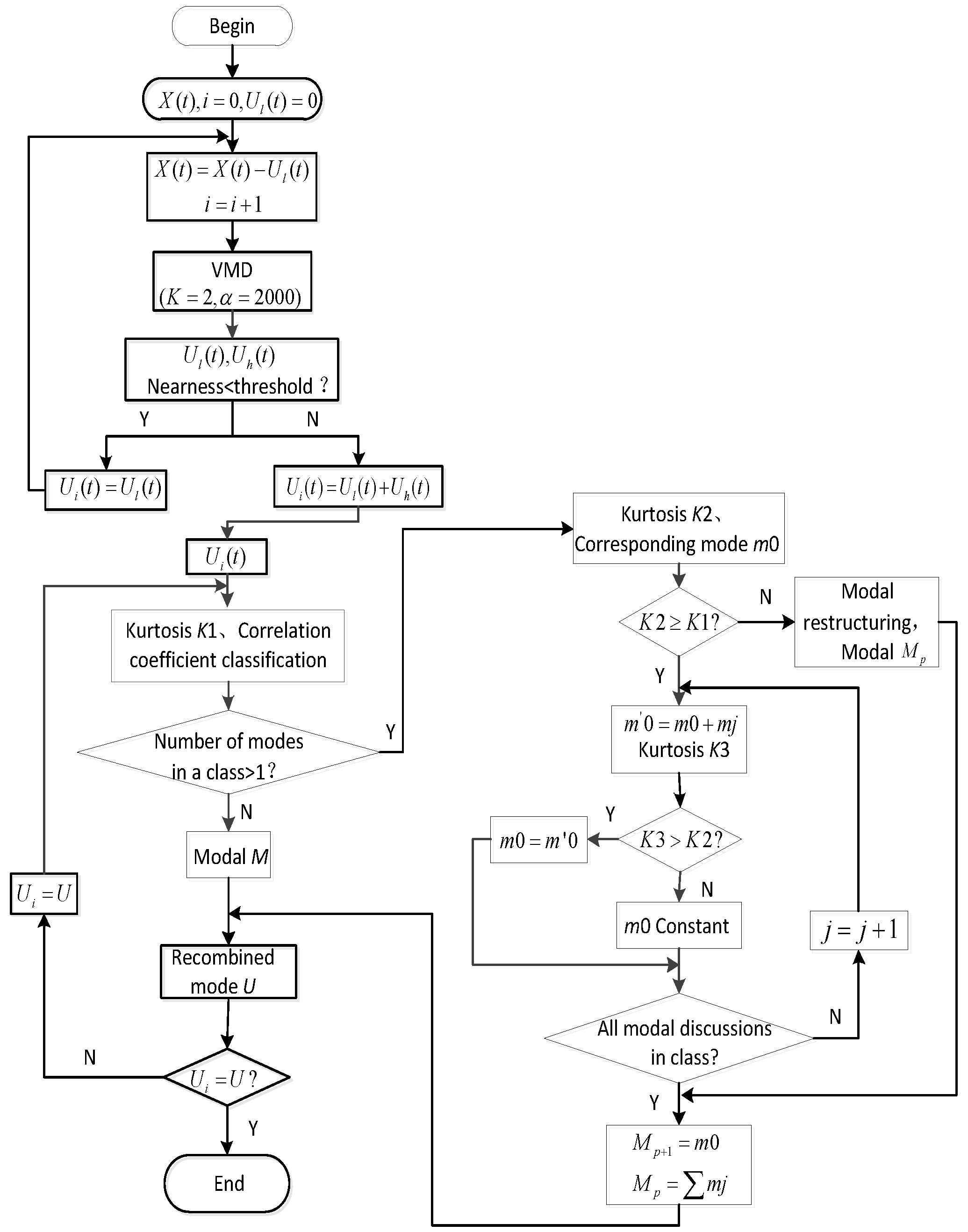
2.1. Improved Variational Mode Decomposition
- (1)
- Initialize and . Assign the original signal to , and assign the low-frequency mode to 0.
- (2)
- Remove low-frequency modes. remove the low-frequency mode from at each run as follows:
- (3)
- Perform VMD decomposition. The number of fixed decompositions K is set to 2, and the penalty factor parameter alpha is set to 2000. The relevant literature showed that the penalty factor demonstrates strong applicability when the penalty factor is set to 2000 and VMD is suitable for extracting low-frequency modal components when the penalty factor is beyond 2000. Therefore, the VMD was run one at a time to obtain both high- and low-frequency modes.
- (4)
- Iteration stop judgment. Stop the iteration when the posting progress of central frequencies of the two modes obtained from the decomposition is less than the set threshold to obtain the final decomposed mode. The posting progress is defined as follows:where and represent the posting progress of center frequencies of modes and , respectively. Step (2) is performed when is less than the set threshold; otherwise, the sum of all low- and high-frequency modes is calculated. Finally, all modes are outputted .
- (5)
- Take the kurtosis. Mode is represented by , and the kurtosis is calculated for all modes . The maximum kurtosis value is denoted as .
- (6)
- Initial mode classification. Fast Fourier transform (FFT) is performed on mode to obtain the corresponding spectrum of each mode as follows:where represents the number of modal components, represents the length of the signal, and represents the amplitude spectrum of modalities. The normalization of obtains as follows:
- (7)
- Modal reorganization determination. On the basis of the kurtosis, the reorganization of the class with more than one mode is determined and the maximum kurtosis S of modes in the class is compared with the value of kurtosis . When , the modal classification in the class is considered to be dominated by noise, the modal reorganization in the class. When , all modalities in the class are combined with corresponding modalities , respectively, and, based on the above principle, the decision is made whether to reorganize or not. Finally, all modalities are outputted after regrouping.
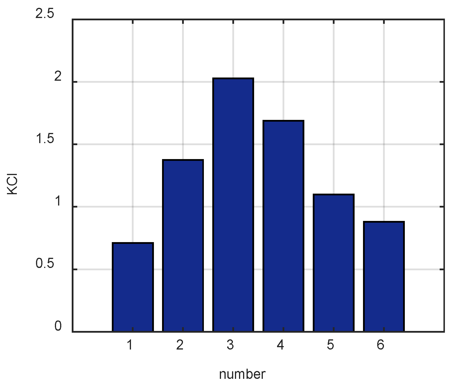
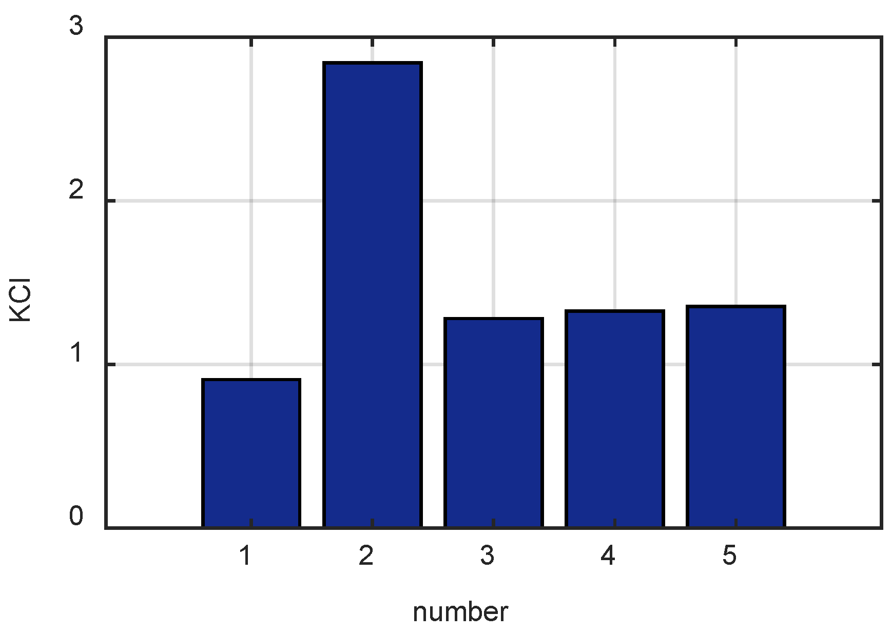
2.2. Mode Selection Based on KCI Features
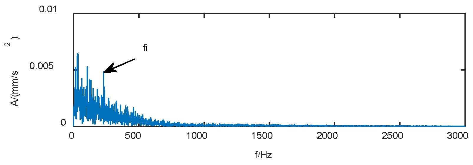
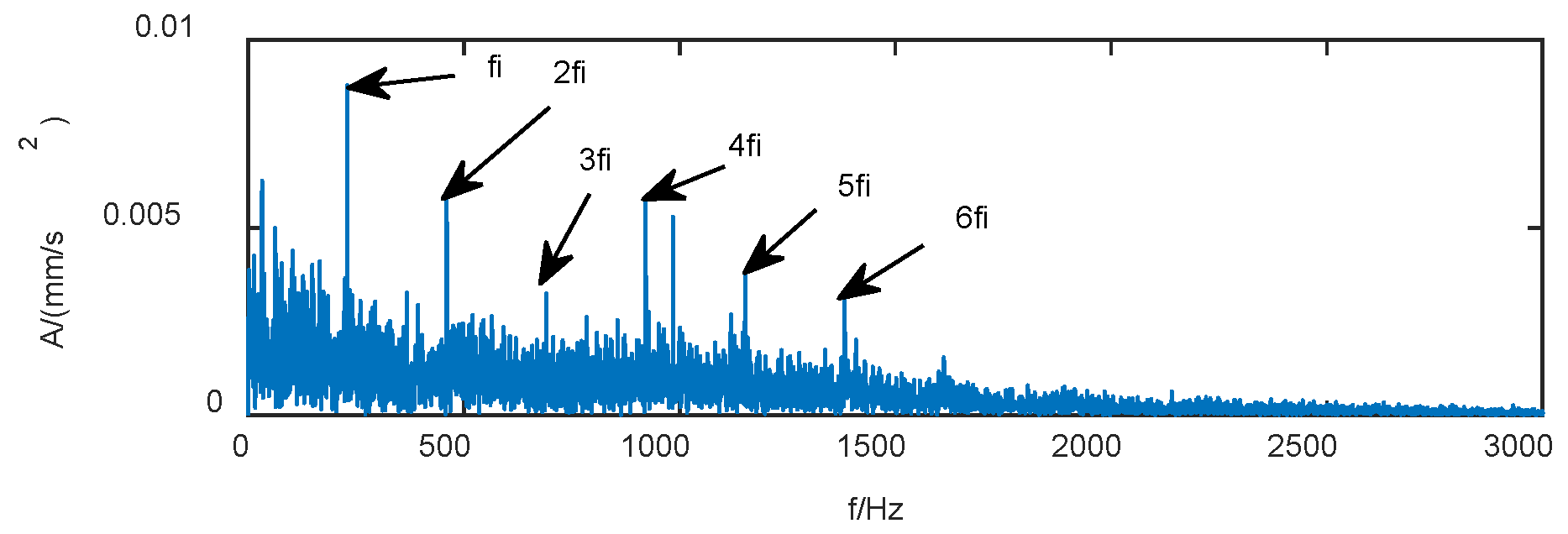
2.3. Defect Frequency Amplitude Ratio
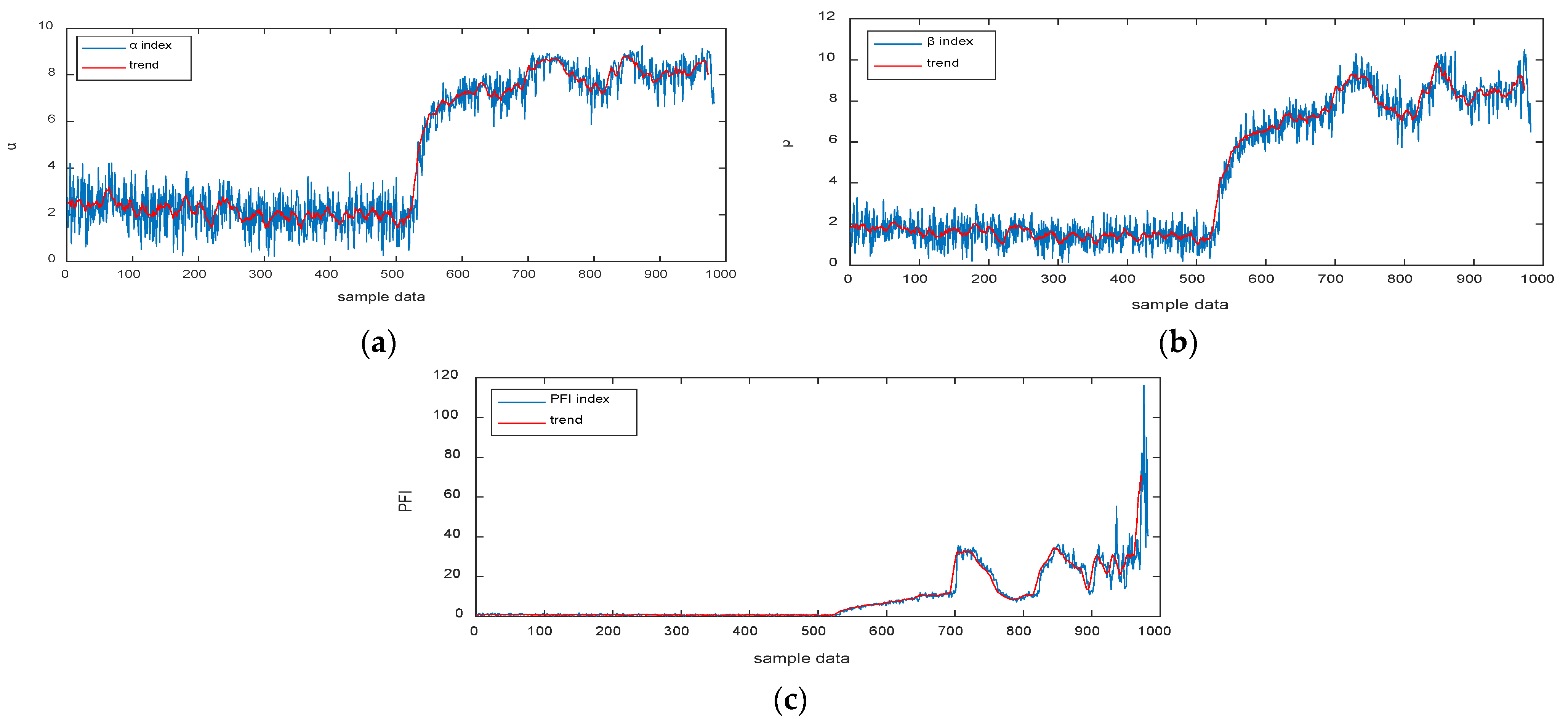
2.4. Comprehensive Indicator Downscaling
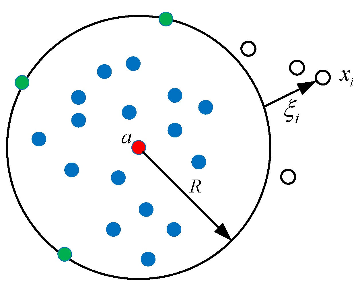
3. Support Vector Data Description
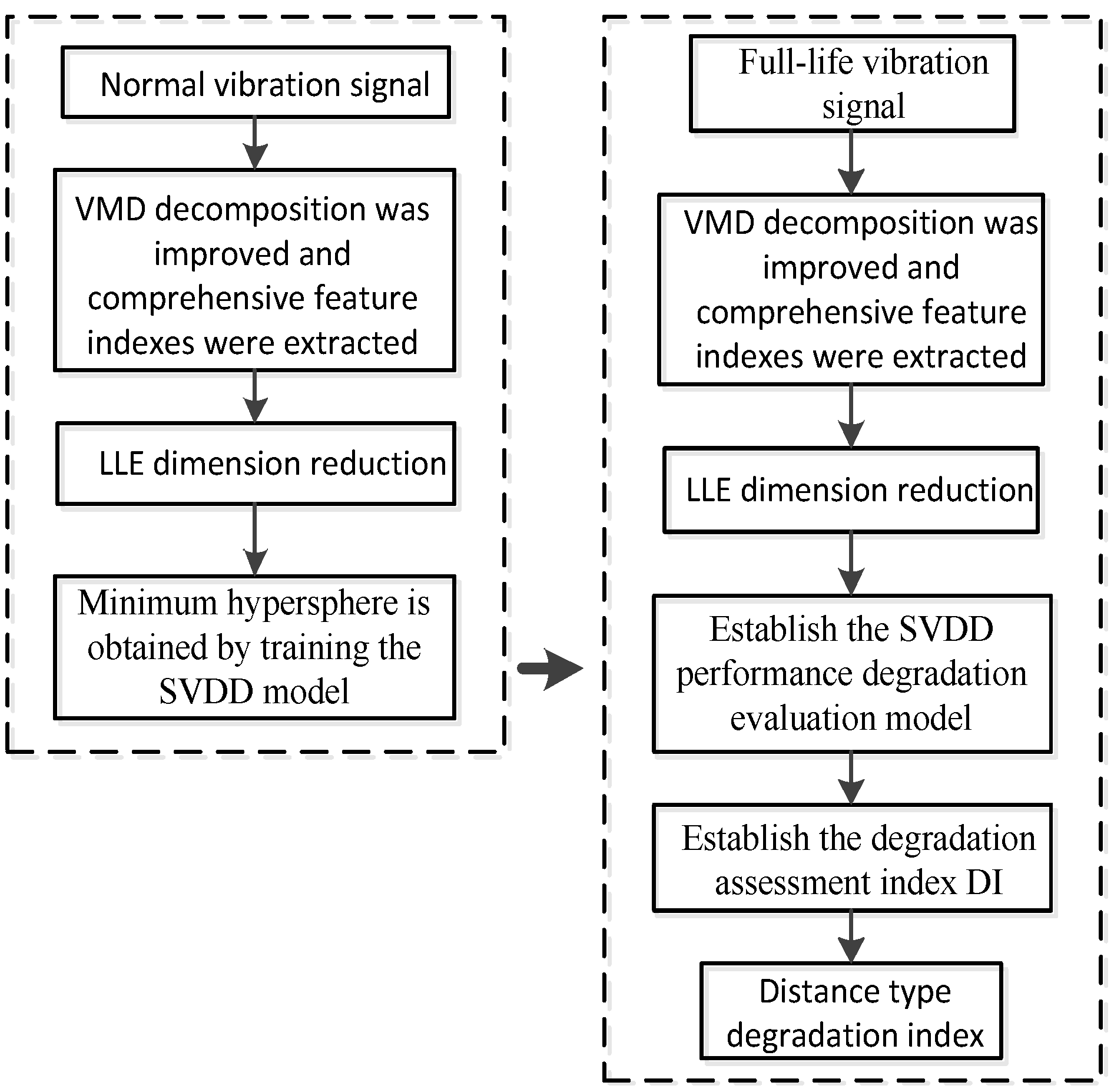
4. Performance Degradation Assessment Based on Combined Metric Downscaling and SVDD

5. Experimental Analysis and Validation
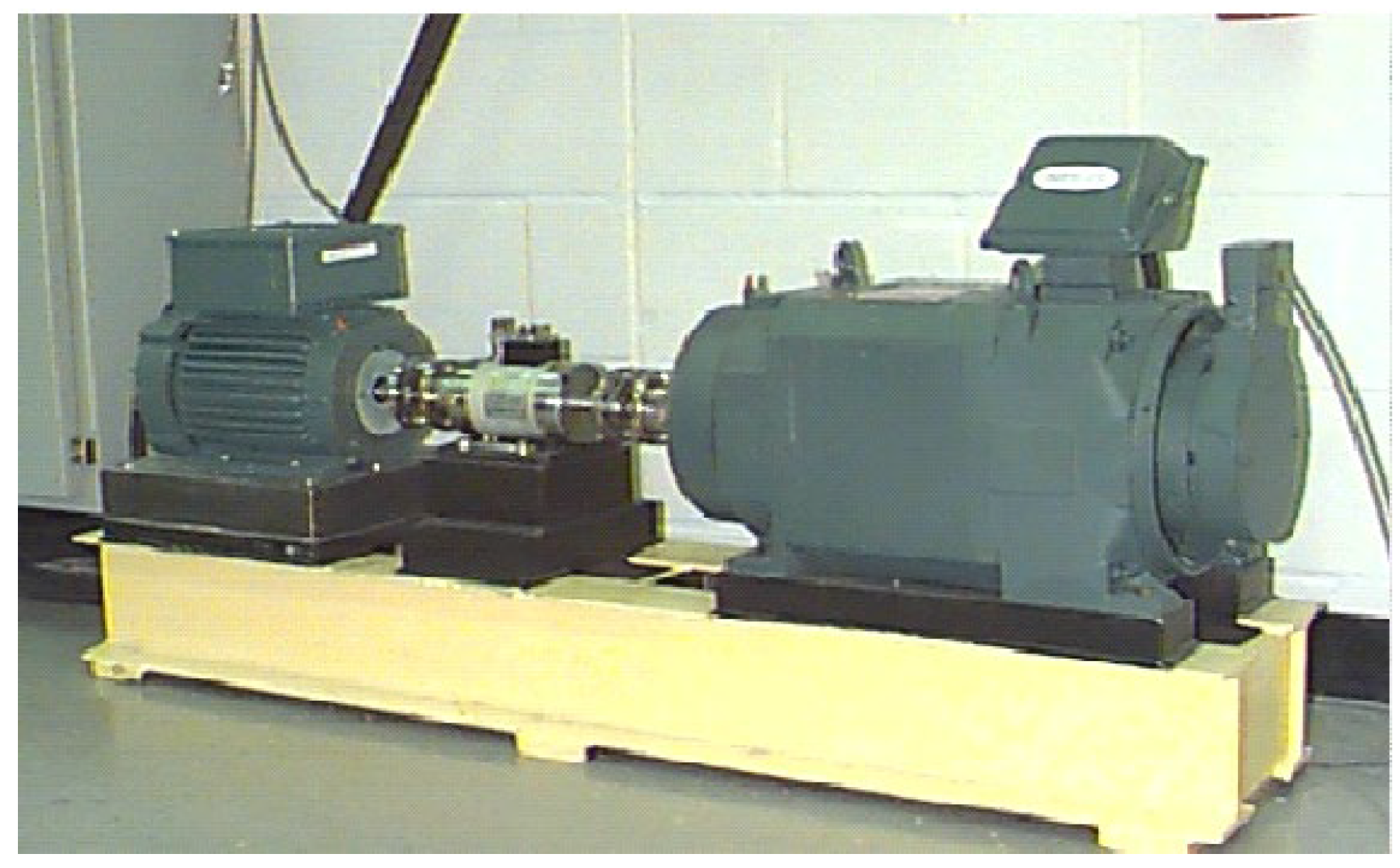
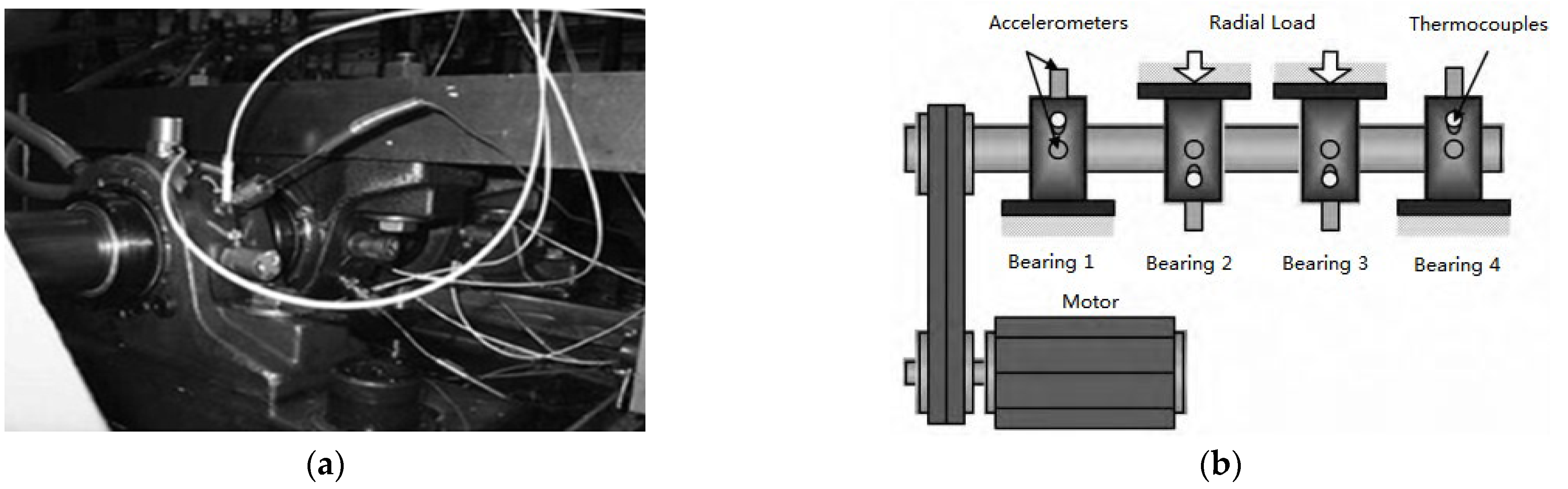
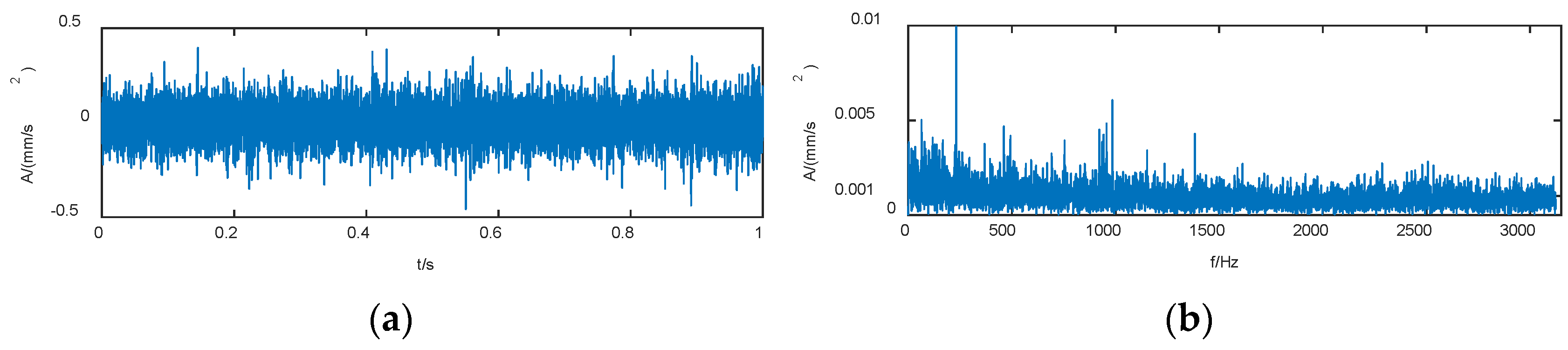
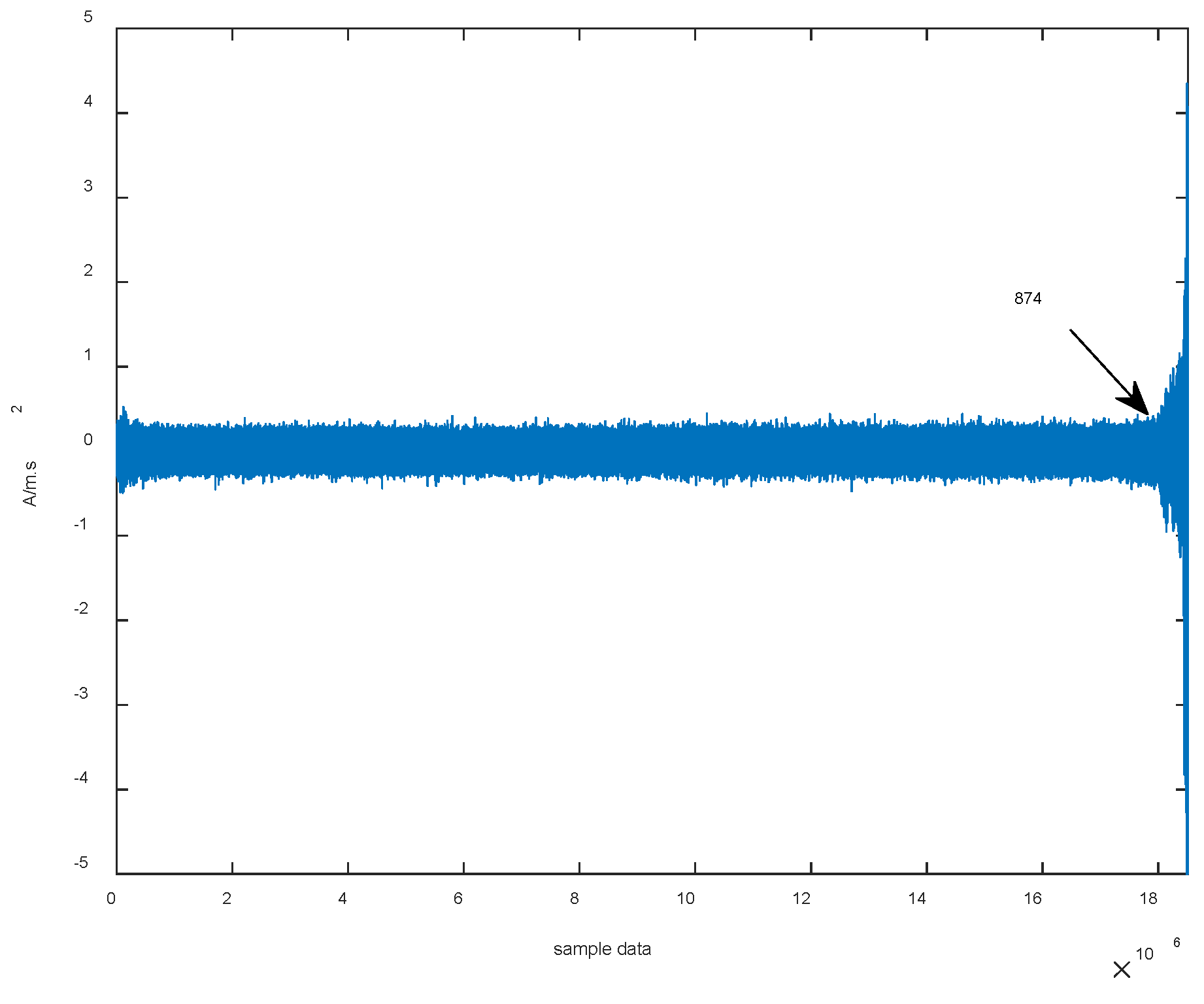
5.1. Presentation of Experimental Data
5.2. Effectiveness of VMD Improvements
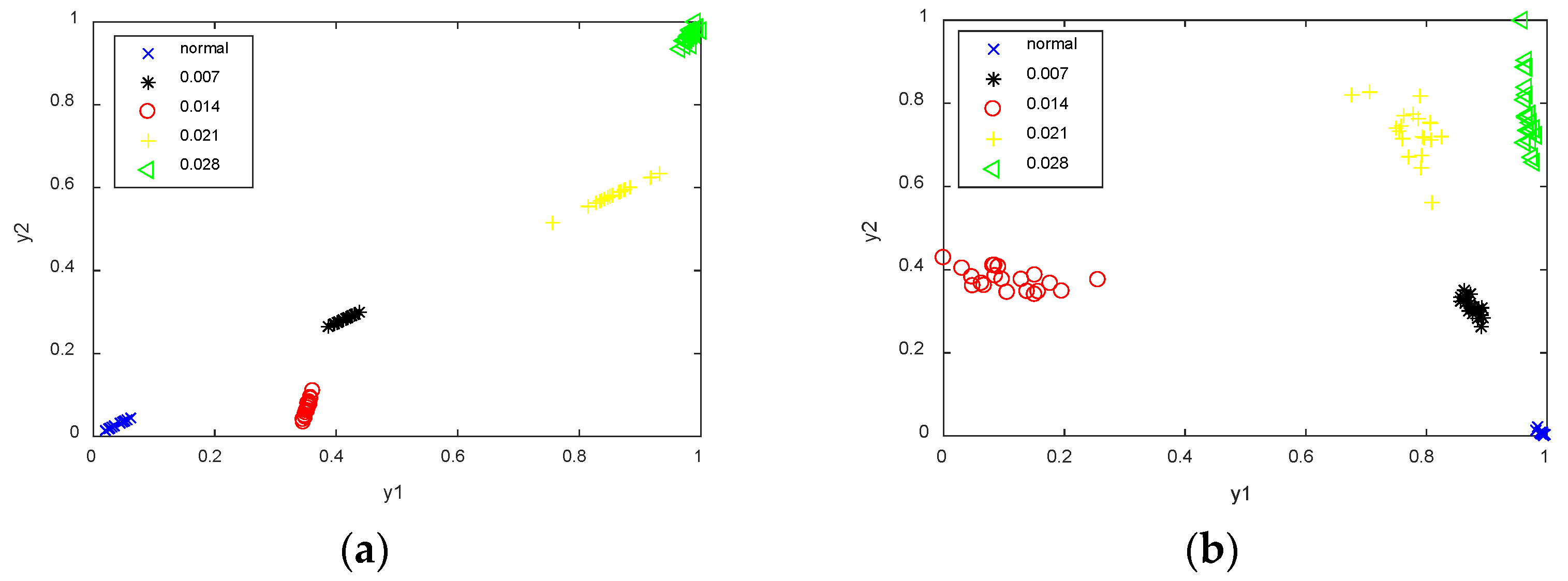
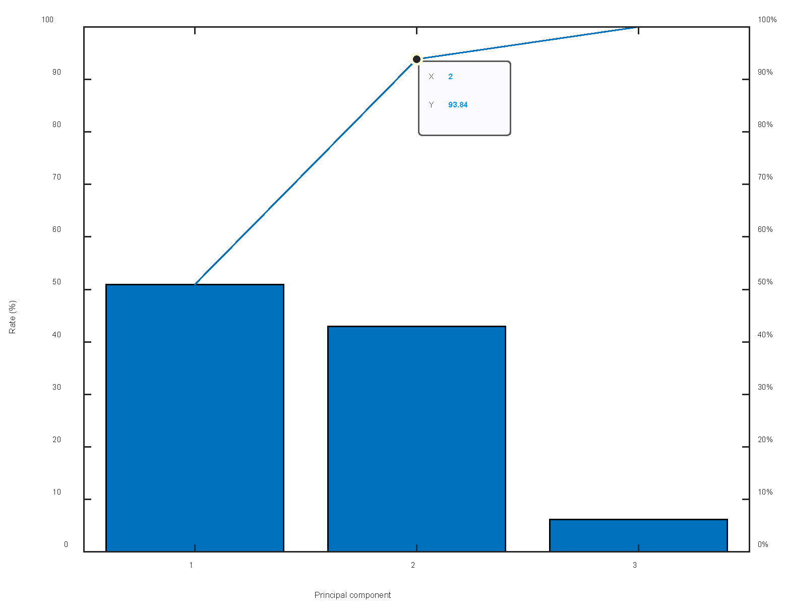
5.3. Comparative Analysis of the Effect of LLE Downscaling
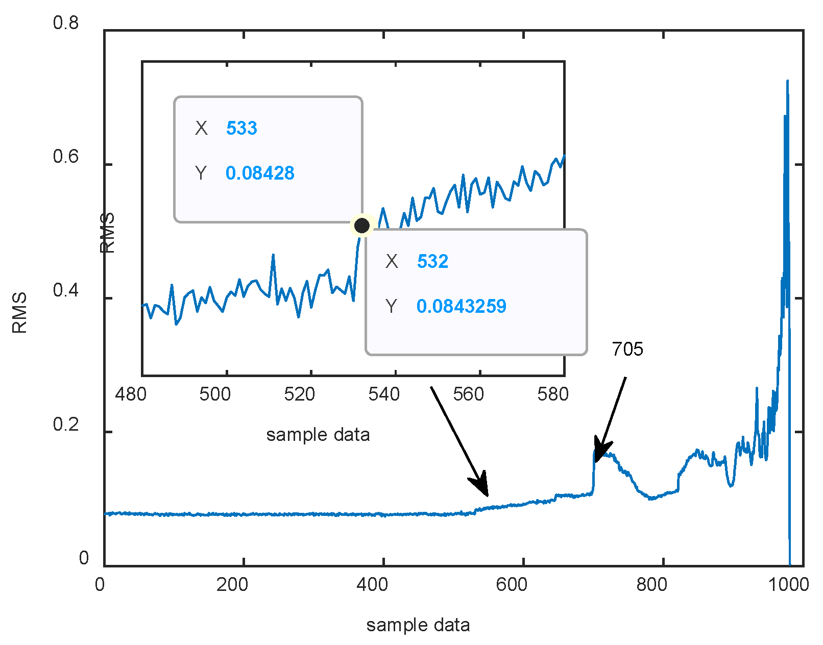
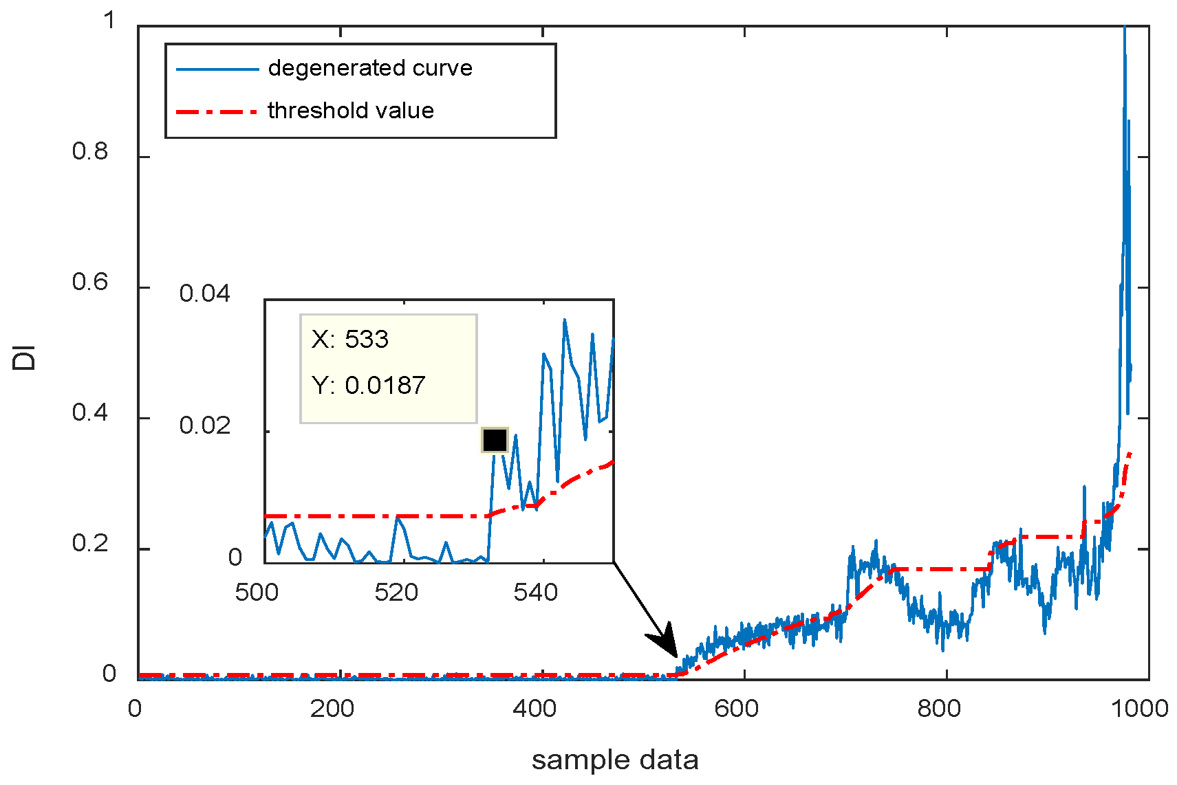
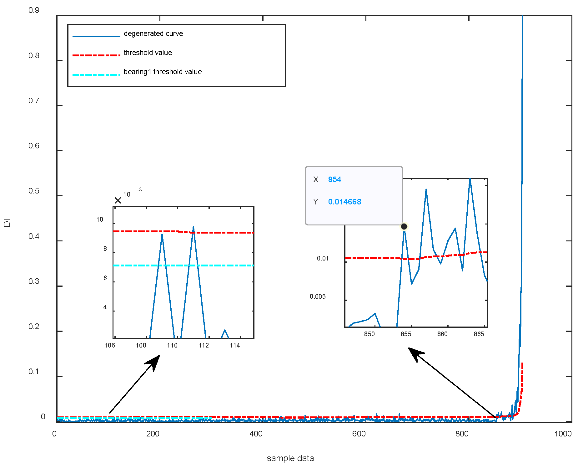
5.4. Assessment of Performance Degradation of Full-Life Rolling Bearings

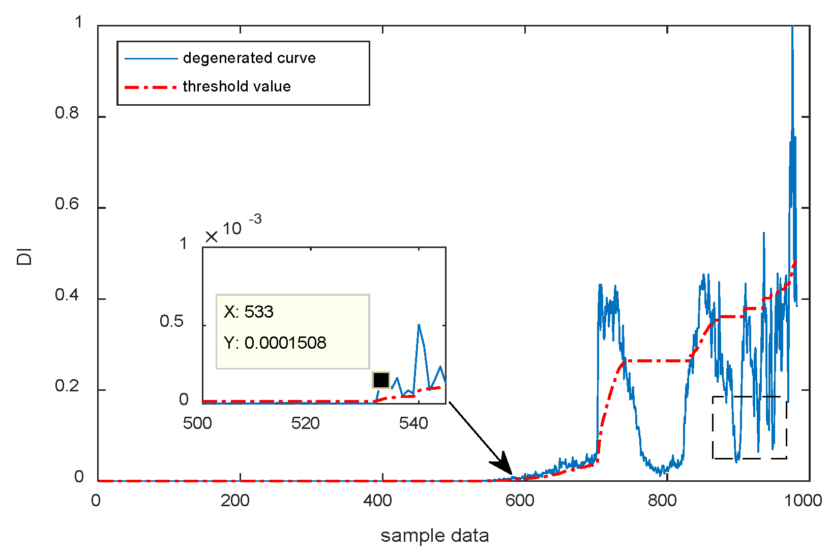
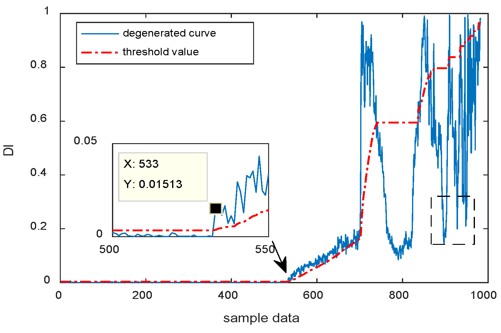
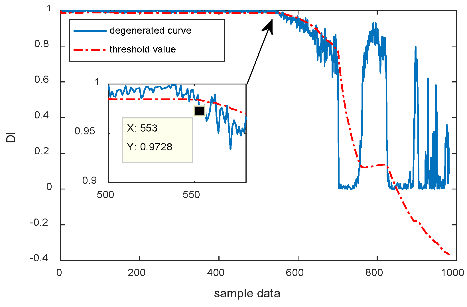
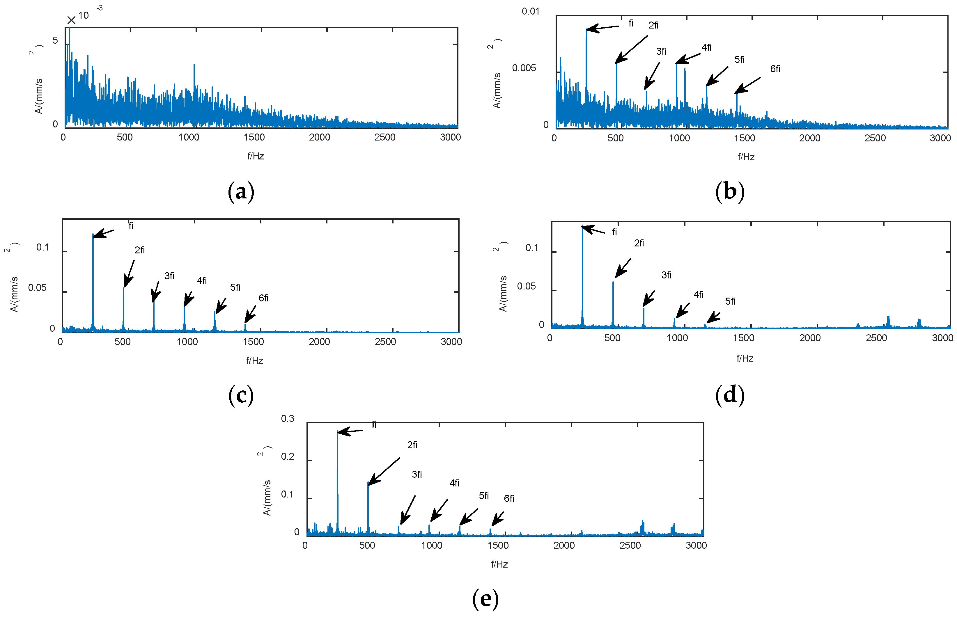
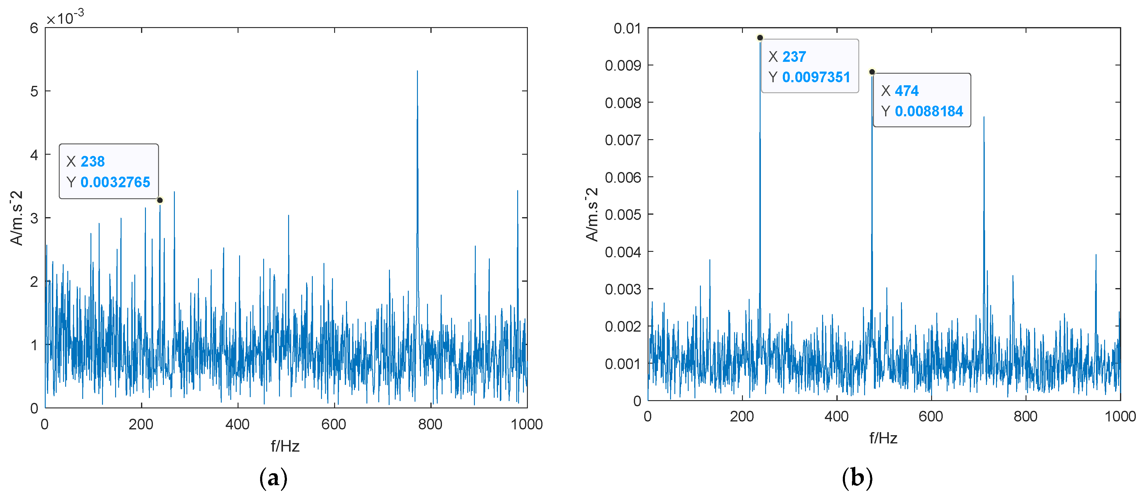
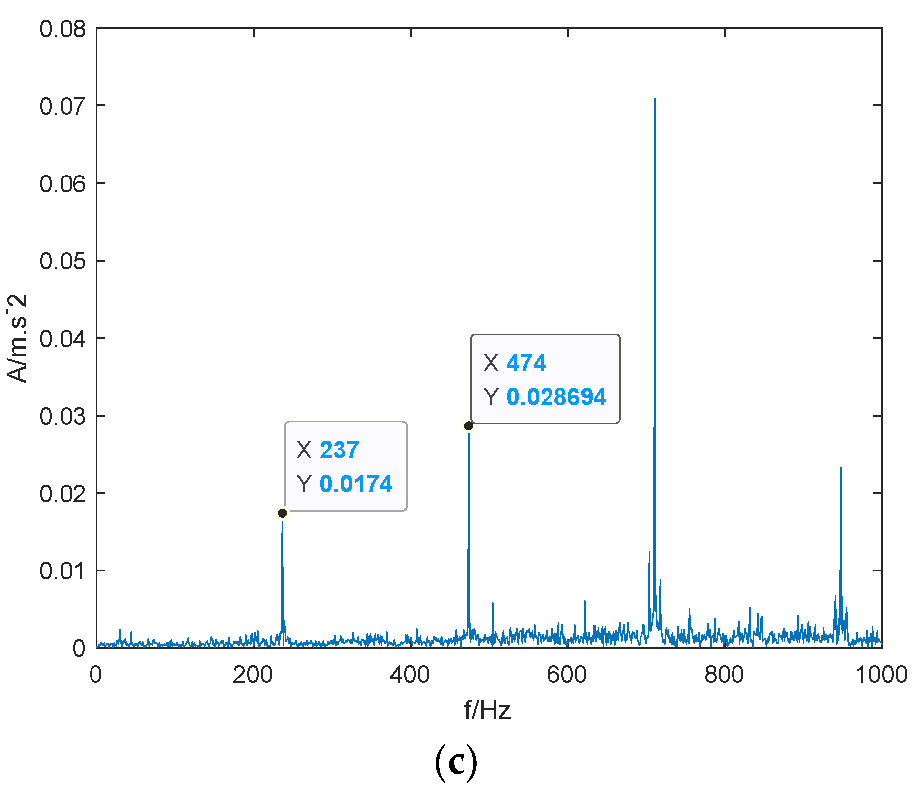
5.5. Fault Verification in All Stages of Bearing Degradation

6. Conclusions
- (1)
- The original vibration signal is decomposed using the improved VMD method, and modalities selected by the weighted kurtosis index are demodulated via enveloping with evident filtering effect. This effect is beneficial for separating early fault characteristics from the disturbance noise and conducive to the extraction of feature indicators.
- (2)
- Defect frequency amplitude ratio indicators, which are sensitive to early faults and more sensitive to early fault onset than traditional RMS indicators, are extracted to address the problem of strong sensitivity of effective feature indicators to the initial stage.
- (3)
- LLE dimensionality reduction is carried out on extracted comprehensive feature indicators to extract the main features, and the SVDD degradation assessment model combined with the relative distance indicator is used in the degradation assessment of the whole-life bearing. The proposed method is important for online health monitoring and early warning of bearings in practical production.
Author Contributions
Funding
Institutional Review Board Statement
Informed Consent Statement
Data Availability Statement
Conflicts of Interest
References
- Li, F.; Chen, Y.; Wang, J.; Zhou, X.; Tang, B. A Reinforcement Learning Unit Matching Recurrent Neural Network for The State Trend Pre-diction of Rolling Bearings. Measurement 2019, 145, 191–203. [Google Scholar] [CrossRef]
- Hu, Y.; Li, H.; Shi, P.; Chai, Z.; Wang, K.; Xie, X.; Chen, Z. A Prediction Method for The Real-time Remaining Useful Life of Wind Turbine Bearings Based on The Wiener Process. Renew. Energy 2018, 127, 452–460. [Google Scholar] [CrossRef]
- Fardin, D.; Myeongsu, K.; Satar, D.; Michael, P. Detection of Generalized-roughness and Single-Point Bearing Faults Using Linear Prediction-based Current Noise Cancellation. IEEE Trans. Ind. Electron. 2018, 65, 9728–9738. [Google Scholar] [CrossRef]
- Cao, L.; Li, J.; Peng, Z.; Han, W.; Zhang, Y. Fault Diagnosis of Rolling Bearing Based on EEMD and Fast Spectral Kurtosis. J. Mech. Eng. 2021, 38, 1311–1316. [Google Scholar]
- Qian, Y.; Yan, R.; Gao, R.X. A Multi-time Scale Approach to Remaining Useful Life Prediction in Rolling Bearing. J. Mech. Syst. Signal Process. 2017, 83, 549–567. [Google Scholar] [CrossRef] [Green Version]
- Randall, R.B.; Antoni, J. Rolling Element Bearing Diagnostics—A Tutorial. Mech. Syst. Signal Process. 2011, 25, 485–520. [Google Scholar] [CrossRef]
- Saidi, L.; Ali, J.B.; Fnaiech, F. Bi-spectrum Based-EMD Applied to The Non-stationary Vibration Signals for Bearing Faults Diagnosis. ISA Trans. 2014, 53, 1650–1660. [Google Scholar] [CrossRef]
- Li, Y.Q.; Wang, R.X.; Xu, M.Q.; Zhou, R.S. A Damage Severity Assessment Method for Bearings with Rolling Element Damage. Shock Vib. 2013, 32, 169–173. [Google Scholar] [CrossRef]
- Yang, T.; Liu, C.; Wu, X.; Liu, X.; Liu, T. Time-domain Compression Feature Extraction and Application Study of Compressed Sensing in Equipment. J. Mech. Eng. Technol. 2017, 36, 1536–1541. [Google Scholar] [CrossRef]
- Zhang, L.; Cheng, L.; Li, X.; Yang, S. Fault Quantitative Evaluation of Rolling Bearings Based on Shock Value of Selected Frequency Band. J. Vib. Shock 2018, 37, 30–38. [Google Scholar] [CrossRef]
- Zhang, L.; Song, C.; Zou, Y.; Hong, C.; Wang, C. Bearing Performance Degradation Assessment Based on Renyi Entropy and K-medoids Clustering. J. Vib. Shock 2020, 39, 24–31. [Google Scholar] [CrossRef]
- Jiang, T.; Zhang, Q. Bearing Failure Impulse Enhancement Method Using Multiple Resonance Band Centre Positioning and Envelope Integration. Measurement 2022, 200, 111623. [Google Scholar] [CrossRef]
- Zheng, J.; Cao, S.; Pan, H.; Ni, Q. Spectral Envelope-based Adaptive Empirical Fourier Decomposition Method and Its Application to Rolling Bearing Fault Diagnosis. ISA Trans. 2022, in press. [CrossRef]
- Kulkarni, V.V.; Khadersab, A. Condition Monitoring Analysis of Rolling Element Bearing Based on Frequency Envelope. Mater. Today Proc. 2021, 46, 4667–4671. [Google Scholar] [CrossRef]
- Xu, X.; Zhao, M.; Lin, J.; Lei, Y. Envelope Harmonic-to-noise Ratio for Periodic Impulses Detection and Its Application to Bearing Diagnosis. Measurement 2016, 91, 385–397. [Google Scholar] [CrossRef]
- Sachan, S.; Shukla, S.; Singh, S.K. Two Level De-noising Algorithm for Early Detection of Bearing Fault Using Wavelet Transform and Zero Frequency Filter. Tribol. Int. 2020, 143, 106088. [Google Scholar] [CrossRef]
- Yu, G.; Li, C.; Sun, J. Machine Fault Diagnosis Based on Gaussian Mixture Model and Its Application. Int. J. Adv. Manuf. Technol. 2010, 48, 205–212. [Google Scholar] [CrossRef]
- Ma, R.; Wang, J.; Song, Y. Multi-manifold Learning Using Locally Linear Embedding (LLE) Nonlinear Dimensionality Reduction. J. Tsinghua Univ. 2008, 48, 582–585. [Google Scholar] [CrossRef]
- Jiang, H.; Chen, J.; Dong, G. Hidden Markov Model and Nuisance Attribute Projection Based Bearing Performance Degradation Assessment. Mech. Syst. Signal Process. 2015, 72–73, 184–205. [Google Scholar] [CrossRef]
- Yu, J.B. Bearing Performance Degradation Assessment Using Locality Preserving Projections and Gaussian Mixture Models. Mech. Syst. Signal Process. 2011, 25, 2573–2588. [Google Scholar] [CrossRef]
- Rai, A.; Upadhyay, S.H. An Integrated Approach to Bearing Prognostics Based on EEMD-multi Feature Extraction, Gaussian Mixture Models and Jensen-Rényi Divergence. Appl. Soft Comput. 2018, 71, 36–50. [Google Scholar] [CrossRef]
- Tong, Q.; Hu, J. Bearing Performance Degradation Assessment Based on Information-theoretic Metric Learning and Fuzzy C-means Clustering. Meas. Sci. Technol. 2020, 31, 075001. [Google Scholar] [CrossRef]
- Wang, F.; Chen, X.; Yan, D.; Li, H.; Wang, L.; Zhu, H. Fuzzy C-means Using Manifold Learning and Its Application to Rolling Bearing Performance Degradation Assessment. J. Manuf. Sci. Eng. 2016, 52, 60–64. [Google Scholar] [CrossRef]
- Jiang, W.; Lei, Y.; Han, K.; Zhang, S.; Su, X. Performance Degradation Quantitative Assessment Method for Rolling Bearings Based on VMD and SVDD. J. Vib. Shock 2018, 37, 43–50. [Google Scholar] [CrossRef]
- Wang, F.; Fang, L.; Zhao, Y.; Qi, Z. Rolling Bearing Early Weak Fault Detection and Performance Degradation Assessment Based on VMD and SVDD. J. Vib. Shock 2019, 38, 224–230. [Google Scholar] [CrossRef]
- Dibaj, A.; Hassannejad, R.; Ettefagh, M.M.; Ehghaghi, M.B. Incipient Fault Diagnosis of Bearings Based on Parameter-optimized VMD and Envelope Spectrum Weighted Kurtosis Index with A New Sensitivity Assessment Threshold. ISA Trans. 2021, 114, 413–433. [Google Scholar] [CrossRef]
- Dragomiretskiy, K.; Zosso, D. Variational Mode Decomposition. IEEE Trans. Signal Process. 2014, 62, 531–544. [Google Scholar] [CrossRef]
- Li, J.; Yao, X.; Wang, H.; Zhang, J. Periodic Impulses Extraction Based on Improved Adaptive VMD and Sparse Code Shrinkage Denoising and Its Application in Rotating Machinery Fault Diagnosis. Mech. Syst. Signal Process. 2019, 126, 568–589. [Google Scholar] [CrossRef]
- Jaskaran Singh, A.K.; Darpe, S.P. Singh. Bearing Damage Assessment Using Jensen-Rényi Divergence Based on EEMD. Mech. Syst. Signal Process. 2017, 87, 307–339. [Google Scholar] [CrossRef]
- Zhang, X.; Wang, H.; Ren, M.; He, M.; Jin, L. Rolling Bearing Fault Diagnosis Based on Multiscale Permutation Entropy and SOA-SVM. Machines 2022, 10, 485. [Google Scholar] [CrossRef]
- Zhou, J.M.; Guo, H.J.; Zhang, L.; Xu, Q.Y.; Li, H. Bearing Performance Degradation Assessment Using Lifting Wavelet Packet Symbolic Entropy and SVDD. Shock Vib. 2016, 2016, 3086454. [Google Scholar] [CrossRef] [Green Version]
- Case Western Reserve University Bearing Data Center Website. Available online: https://engineering.case.edu/bearingdatacenter/welcome (accessed on 7 July 2022).
- Lee, J.; Qiu, H.; Yu, G.; Lin, J.; Rexnord Technical Services. IMS, University of Cincinnati. “Bearing Data Set”, NASA Ames Prognostics Data Repository. NASA Ames Research Center, Moffett Field, CA, USA. 2007. Available online: https://ti.arc.nasa.gov/progect/prognostic-data-repository (accessed on 7 July 2022).
- Qiu, H.; Lee, J.; Lin, J.; Yu, G. Wavelet Filter-based Weak Signature Detection Method and Its Application on Rolling Element Bearing Prognostics. J. Sound Vib. 2006, 289, 1066–1090. [Google Scholar] [CrossRef]
- Gu, R.; Chen, J.; Hong, R. Early Fault Diagnosis of Rolling Bearings Based on Adaptive Variational Mode Decomposition and The Teager Energy Operator. J. Vib. Shock 2020, 39, 1-7+22. [Google Scholar] [CrossRef]
- Zhang, L.; Huang, W.; Xiong, G.; Cao, Q. Assessment of Rolling Bearing Performance Degradation Using Gauss Mixture Model and Multi-domain Features. J. China Mech. Eng. 2014, 25, 3066–3072. [Google Scholar] [CrossRef]


| Method | VMD | Improvement of VMD |
|---|---|---|
| PSNR | 19.627 | 22.495 |
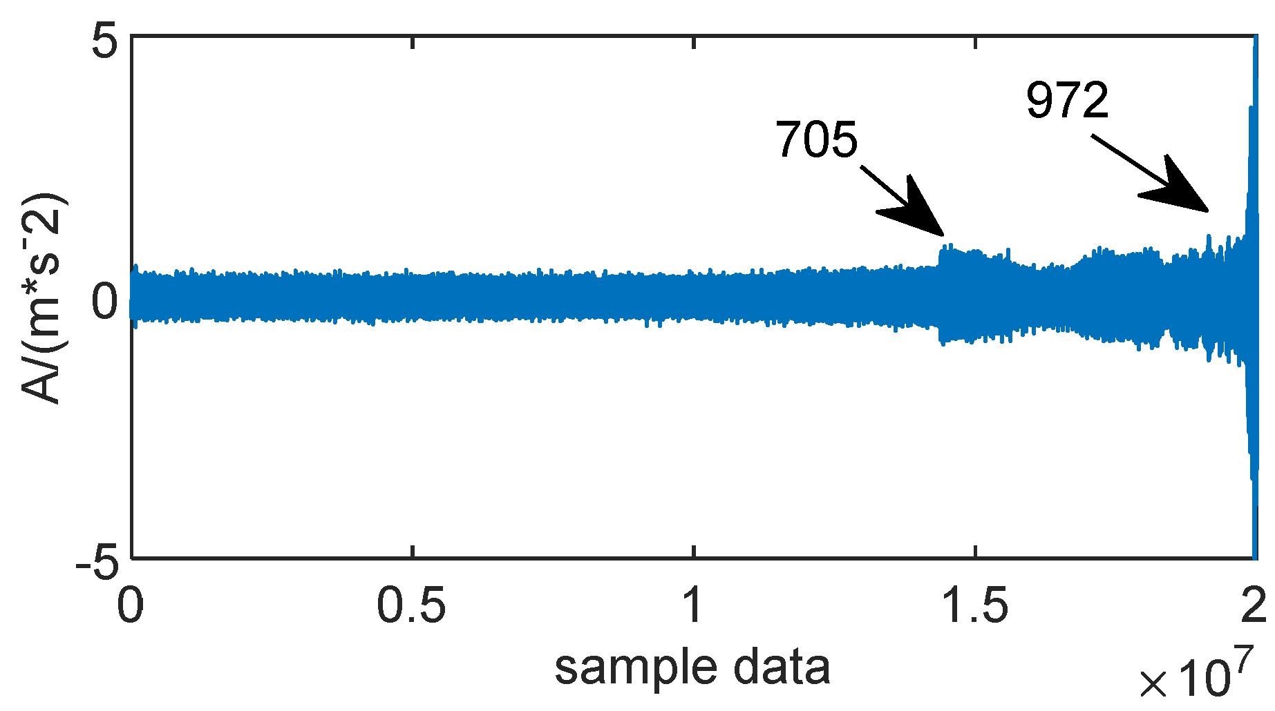
| Sample point | 533rd | 705th | 850th | 972nd |
| Amplitude | 0.0087 | 0.1215 | 0.135 | 0.2787 |
| Bearing condition | Early failure | Medium failure | Severe failure | Very severe failure |
Publisher’s Note: MDPI stays neutral with regard to jurisdictional claims in published maps and institutional affiliations. |
© 2022 by the authors. Licensee MDPI, Basel, Switzerland. This article is an open access article distributed under the terms and conditions of the Creative Commons Attribution (CC BY) license (https://creativecommons.org/licenses/by/4.0/).
Share and Cite
Xin, H.; Zhang, H.; Yang, Y.; Wang, J. Evaluation of Rolling Bearing Performance Degradation Based on Comprehensive Index Reduction and SVDD. Machines 2022, 10, 677. https://doi.org/10.3390/machines10080677
Xin H, Zhang H, Yang Y, Wang J. Evaluation of Rolling Bearing Performance Degradation Based on Comprehensive Index Reduction and SVDD. Machines. 2022; 10(8):677. https://doi.org/10.3390/machines10080677
Chicago/Turabian StyleXin, Hongwei, Haidong Zhang, Yanjun Yang, and Jianguo Wang. 2022. "Evaluation of Rolling Bearing Performance Degradation Based on Comprehensive Index Reduction and SVDD" Machines 10, no. 8: 677. https://doi.org/10.3390/machines10080677