Integrated Path Tracking and Lateral Stability Control with Four-Wheel Independent Steering for Autonomous Electric Vehicles on Low Friction Roads

Abstract

This paper presents a method to design an integrated path tracking and lateral stability controller for an autonomous electric vehicle with four-wheel independent steering (4WIS) on low friction roads. Recent advances in autonomous driving have led to extensive studies on path tracking control. However, path tracking is difficult on low friction roads. In this paper, path tracking control was converted to the yaw rate tracking one to cope with problems caused by low friction roads. To generate a reference yaw rate for path tracking, we present several methods using a driver model and a target path. For yaw rate tracking, we designed a controller with a two-layer control hierarchy, i.e., upper and lower layers. The control yaw moment was calculated using a direct yaw moment controller in the upper layer. In the low layer, a control allocation method was adopted to allocate the control yaw moment into steering angles of 4WIS. To verify the performance of the proposed controller, we conducted a simulation on vehicle simulation software. From the simulation results, it is shown that the proposed controller is effective for path tracking and lateral stability on low friction roads. To analyze path tracking and lateral stability performance of the proposed controller on low friction roads, the effects of the steady-state yaw rate gain are investigated from the simulation results.

1. Introduction

Over the last decade, autonomous driving has been expected as a solution for future transportation in the automotive industry. Particularly, road safety, traffic flow, and passenger convenience can be improved by the aid of autonomous driving [1,2,3]. For example, in view of road safety, about 92% of road crashes occurred mainly due to human errors [4,5]. In view of traffic flow, current road infrastructure is not operated at its maximum capacity due to vehicles driven by human drivers. More specifically, only 11% of the road lane length of highways is occupied by vehicles while the remaining 89% is an inter-vehicle gap needed for drivers to feel safe when driving at high speeds [6]. On the contrary, in view of passenger comfort, excessive small inter-vehicle gaps can cause discomfort to passengers [7]. Under those situations, autonomous driving has been regarded as the most promising solution to these problems. As a consequence, autonomous driving has been extensively studied.

According to the literature on autonomous driving, information flow for autonomous driving consists of localization and mapping, perception, assessment, planning and decision making and control [2]. Among them, this paper concentrates on control, especially path tracking control. As a result of the expectation to autonomous driving, a lot of papers have been published on path tracking control for autonomous vehicles [8,9,10,11,12,13,14]. In the literature on path tracking control, linear quadratic regulator (LQR), H_∞ control, sliding mode control (SMC) and model predictive control (MPC) have been adopted as a controller design methodology. Most of these papers have used error dynamics derived from a target path, which the lateral offset and heading errors of a vehicle were used to define the error dynamics [12]. However, in the case of using the error dynamics, assumptions on a target path are required. The most important assumption on a target path requires that the path is smooth or differentiable. For this reason, the error dynamics-based method cannot generate a steering angle if there are sharp corners or non-differentiable points on a target path. As a consequence, it is difficult for the error dynamics-based method to guarantee path tracking performance in various driving conditions. For this reason, simple methods such as a pure pursuit method or Stanley method have been widely used as a path tracking controller for autonomous vehicles. To cope with the problem of the error dynamics-based method, it is necessary to design a path tracking controller that does not need the error dynamics on a target path.

Besides the problems of the error dynamics-based method, there have been few papers that have concentrated on path tracking control on low friction roads. Generally, a friction circle, whose the radius is calculated as the multiplication of the tire-road friction coefficient and vertical tire force, imposes a limit on the maximum available longitudinal and lateral tire forces of a vehicle. On low friction roads, the radius of a friction circle is reduced. As a consequence, the maximum available longitudinal and lateral forces generated on tires in a vehicle are reduced. Figure 1 shows the lateral tire forces with respect to the tire slip angle and the tire-road friction coefficient. As shown in Figure 1, the lateral tire force is reduced as the tire-road friction coefficient decreases. Due to reduced lateral tire forces, a path tracking controller, designed on high friction roads, becomes ineffective on low friction roads. In other words, the path tracking performance of a controller designed on high friction roads deteriorates on low friction roads. For this reason, it is necessary to design a path tracking controller considering low friction road conditions.

In the area of active safety for vehicles, vehicle stability control (VSC) has been studied since the mid-1990s [15,16,17,18]. There are two objectives in vehicle stability control [17]. The first is to make a vehicle to follow a reference yaw rate, which represents driver’s intention. This is called maneuverability. The second is to maintain the side-slip angle of a vehicle as small as possible. This is called lateral stability. As pointed out by Wong, it is necessary to maintain the lateral stability on low friction roads because the lateral stability is not maintained although the maneuverability is satisfied [19]. In view of the actuator for VSC, several actuators have been used [17]. A typical actuator for VSC is electronic stability control (ESC), which has independent or differential braking [15]. In this paper, ESC is called 4-wheel independent braking (4WIB). Steering-based actuators used for VSC are active front steering (AFS), rear-wheel steering (RWS) and 4-wheel steering (4WS) [20]. These actuators have the advantage over ESC because it does not use braking, which causes speed reduction [17]. Another actuator for VSC is torque vectoring device (TVD) or 4-wheel drive (4WD) [21]. For the last decade in the area of VSC, there have been a lot of papers published on vehicle stability control with multiple actuators such as ESC, AFS and TVD. This is called unified chassis control (UCC) or integrated chassis control (ICC) [17].

By virtue of recent electrification on a vehicle, the powertrain of a vehicle has been drastically changed over the last two decades. In view of an actuator, an in-wheel motor (IWM) has been developed as a future powertrain for electric vehicles [22]. Basically, an electric vehicle equipped with IWM (EV-IWM) has 4-wheel independent steering (4WIS) and driving (4WID) functions. If an electro-mechanical brake (EMB) is adopted as a brake system for IWM, EV-IWM has 4-wheel independent braking (4WIB) function [23]. To date, there have been few papers on ICC or VSC for EV-IWM with 4WIS, 4WID and 4WIB [20,23].

Generally, most path tracking controllers have been designed for a front wheel steering (FWS) vehicle. By virtue of recent advances in actuators for VSC in EV-IWM, 4WS, 4WIS and 4WID have been widely adopted for path tracking control [24,25,26,27,28,29,30,31,32,33,34,35,36,37,38,39,40,41]. Among them, a lot of papers have been published on the path tracking control for a vehicle with 4WS and/or 4WD [24,26,27,28,29,32,33,34,38,41]. On the other hand, there have been few studies on the path tracking control for a vehicle with 4WIS and/or 4WID for autonomous EV-IWM (AEV-IWM) [25,30,31,35,36,37,39,40]. In general, it is difficult to determine the steering angles of 4WIS from the methods used for path tracking control on FWS vehicles. In previous studies, path tracking controllers were designed for vehicles with 4WS [29,31,39,41]. In these studies, the steering angles of 4WS were obtained with LQR and MPC, and then converted to the steering angles of 4WIS by using a geometrical relationship. However, there were few differences between 4WS and 4WIS in these studies. To cope with this problem, some papers proposed the idea that the path tracking control is converted to the yaw rate tracking one, which has been widely adopted for VSC [30,36,37,40]. In the area of VSC, the yaw rate tracking or vehicle stability controller has been designed for a vehicle with 4WIS, 4WID and 4WIB [20,23]. For this reason, the yaw tracking control for AEV-IWM with 4WIS has been applied to the path tracking control.

To date, there have been few studies on the path tracking control on low friction roads. Since 2015, some papers on the topic have been published [42,43,44,45,46,47,48,49]. Most of these papers have used an error dynamics-based model for controller design, and adopted LQR, SMC and MPC as a controller design methodology. Typical tire-road friction coefficient used in these studies is between 0.3 and 0.4. Typical actuators used in these studies are AFS/4WIB and 4WD/4WID. As mentioned earlier, the lateral stability should be maintained on low friction roads [19]. As a measure of the lateral stability, the side-slip angle has been used [17,18,20]. Generally, it has been known that path tracking and lateral stability cannot be satisfied simultaneously on low friction roads. For this reason, most of these papers have adopted a coordination scheme between path tracking and lateral stability [46,49,50]. However, there are scarce studies investigating the coordination between path tracking and lateral stability for AEV-IWM with 4WIS on low friction roads. For this reason, this paper concentrates on how to coordinate path tracking and lateral stability on low friction roads for AEV-IWM with 4WIS.

This paper presents a method to design an integrated path tracking and stability controller for AEV-IWM with 4WIS on low frictions roads. Figure 2 shows the schematic diagram of the proposed integrated controller. As shown in Figure 2, the proposed integrated controller comprises two modules: Reference Yaw Rate Generation and Yaw Rate Tracking Controller. In this paper, the path tracking control problem is converted to the yaw rate tracking one that has been used for vehicle stability control [30,36,37,40]. In Figure 2, the Reference Yaw Rate Generation module generates the reference yaw rate for the path tracking control. For this purpose, two types of methods were adopted: a driver model and a path-based method. In Figure 2, the Yaw Rate Tracking Controller module generates the steering angles of 4WIS from the reference yaw rate. The proposed controller has two-layer structure: the upper and lower layers [17,20,23]. A control yaw moment is calculated with direct yaw moment control in the upper layer. In the lower layer, by using a control allocation method, the control yaw moment is distributed into lateral tire forces at each wheel. From the lateral tire forces obtained from the control allocation, the steering angles of 4WIS are determined with the definition of slip angles [17,20,23]. To verify the performance of the proposed integrated path tracking and lateral stability controller, a simulation is conducted on vehicle simulation software, CarSim [51]. From the simulation results, it is shown that the proposed controller is effective in improving the path tracking while maintaining the lateral stability of AEV-IWM on low friction roads. To analyze the path tracking and lateral stability of the proposed controller on low friction roads, the effects of the steady-state yaw rate gain are investigated from the simulation results.

The key contributions in this paper are summarized as follows:

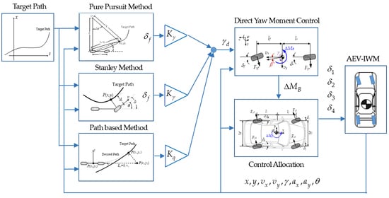
• In this paper, we converted the path tracking control to the yaw rate tracking one in order to fully utilize 4WIS for path tracking. It was difficult to determine the steering angles of 4WIS by virtue of the methods used for path tracking control on FWS vehicles. In this paper, with the aid of control allocation in the yaw rate tracking control, the path tracking controller was designed for an autonomous electric vehicle with 4WIS.
• For path tracking on low friction roads, we designed a yaw tracking controller guaranteeing lateral stability with 4WIS. With this manner, the path tracking control was integrated with lateral stability control.
• This paper shows that a coordination or switching scheme between path tracking and lateral stability on low friction roads was not needed under a particular controller structure and parameter setting.

This paper consists of five sections. Section 2 presents driver models used to generate the steering angle and the methods to derive the reference yaw rate from it. In Section 3, the proposed integrated controller with the upper- and lower-level layers is explained. Simulation is conducted and simulation results are analyzed in Section 4. In Section 5, the conclusion of this research is given.

2. Derivation of Reference Yaw Rate

As mentioned earlier, the path tracking control problem is converted to the yaw rate tracking one in this paper [30,36,37,40]. The yaw rate tracking control is defined as a control that tries to make a vehicle follow the reference yaw rate. Therefore, it is necessary to generate the reference yaw rate for path tracking. For the purpose, two driver models and a path-based method are presented in this section.

2.1. Driver Models

The typical method used for a driver model in autonomous driving is the pure pursuit method. Figure 3 shows the illustration for the pure pursuit method [13]. In Figure 3, P(x,y) is the target point and φ is the heading angle between the vehicle’s heading vector and the look-ahead direction. L_p and R are the look-ahead distance and the radius of the circular arc, respectively. Generally, basic chassis sensors have been installed on real vehicle in order to measure wheel speed, steering angle, yaw rate, and longitudinal and lateral acceleration. Moreover, the position and heading information, i.e., P(x,y) and the current position of a vehicle, can be obtained from SLAM algorithms with various sensors such as DGPS, IMU, LiDAR, and camera and filters, all of which are generally used for autonomous driving [52]. In Figure 3, the point O is the instantaneous center of the circular arc on the vehicle motion. The turning radius R can be calculated from φ and L_p. With R and the position information of the vehicle, the point O is obtained from the rear axle and P(x,y), as shown in Figure 3. In the pure pursuit method, the steering angle of front wheels is calculated only from P(x,y) and φ. From Figure 3, the curvature κ of the circular arc connecting P(x,y) and the rear wheel is calculated, as is shown in Equation (1). With the definition of κ, the steering angle of front wheels, δ_f, is calculated, as is shown in Equation (2) [13]. In Equation (2), L is the wheelbase. As is shown in Figure 3, the look-ahead distance is proportional to the longitudinal speed, v_x, where k_p is the parameter used to tune the look-ahead distance. Generally, k_p is set between 1 and 2 secs according to vehicle speeds. If this value becomes smaller than 1 sec, it represents an inexperienced driver, which generates a larger steering angle from a shorter look-ahead distance [17,20]. In this paper, k_p is set to 0.8 sec because a larger steering angle is needed for path tracking on low friction roads.

$$\kappa =\frac{1}{R}=\frac{2\sin \phi }{L_p}$$

(1)

$${\delta }_f={\tan }^{-1}\left(\kappa L\right)={\tan }^{-1}\left(\frac{2L\sin \phi }{L_p}\right)={\tan }^{-1}\left(\frac{2L\sin \phi }{k_p\cdot v_x}\right)$$

(2)

Another method used as a driver model in autonomous driving is the Stanley method. The Stanley method is a path tracking controller developed by Stanford University’s autonomous vehicle entry in the DARPA Grand Challenge, Stanley [53]. Figure 4 shows Stanley method geometry, i.e., the geometric relationship among control parameters of Stanley method. For the Stanley method, two errors are defined: the heading and lateral offset errors. The heading error, θ_e, is defined as the difference between the heading angles of the vehicle and the path at P(x,y), as shown in Figure 4. The lateral offset or distance error, d_e, is defined as the distance from the center of the front axle to the nearest point P(x,y) on the target path. The Stanley method consists of two terms corresponding to two errors. The first term makes the direction of wheels aligned with the given path by setting the front steering angle equal to θ_e. The second term adjusts δ_f such that the intended trajectory intersects the path tangent from P(x,y) at k⋅v units from the front axle if d_e is non-zero. In Equation (3), k_s is a gain parameter used to tune the magnitude of the distance error. In this paper, k_s is set to 1.0, which is selected by trial and error through simulation. The final steering angle of front wheels, δ_f, is obtained as the sum of these two terms, as given in Equation (3). It is obvious that the desired motion is achieved with this method: As d_e increases, the front wheels are steered further towards the target path.

$${\delta }_f={\theta }_e+{\tan }^{-1}\left(\frac{k_s\cdot d_e}{v}\right)$$

(3)

The PID driver model is an extension of the Stanley method, which applies proportional (P), integral (I), and derivative (D) control to the heading and distance errors in the Stanley method. In other words, the Stanley method is P-controller with heading and distance errors. However, it is not easy to tune the six gains of the PID driver model, which has poor versatility [12]. For this reason, this paper did not adopt the PID driver model.

The above two driver models generate the steering angle of front wheels for a vehicle with FWS. For the reason, these methods are not relevant to an AEV-IWM with 4WIS. To use these methods for an AEV-IWM with 4WIS, the path tracking control should be converted to the yaw rate tracking control because it is easy to use 4WIS in the yaw rate tracking control [30,36,37,40]. The next step after steering angle generation is to calculate the reference yaw rate with the steering angle of the driver models.

2.2. Calculation of the Reference Yaw Rate from the Steering Angle

In the literature on the yaw tracking control, the reference yaw rate has been calculated from the steering angle of front wheels generated by a driver, which represents the driver’s intention. When calculating the reference yaw rate, the most widely used method is based on the steady-state motion of a bicycle model [19,54]. Figure 5 shows 2-DOF bicycle model, which describes the yaw and lateral motions under the assumption that the longitudinal velocity v_x is constant [17,18,19,20,23,54]. In this model, there are two dynamic variables: the yaw rate, γ, and the lateral velocity, v_y. With the dynamic variables, the equations of motions for the model are derived as shown in Equation (4) [19,54]. In Equation (4), β is the side-slip angle, which is defined as v_y divided by v_x. Tire slip angles of the front and rear wheels, α_f and α_r, are defined in Equation (5) using γ, v_y, and v_x. In Equation (4), the lateral tire forces of the front and rear wheels, F_yf and F_yr, are assumed to be proportional to the tire slip angles, as given in Equation (6), respectively. The reference yaw rate, γ_d, is calculated in Equation (7) from steady-state relation between steering angle and radius of vehicle trajectory [54]. In Equation (7), K_γ is the steady-state yaw rate gain used as a multiplication factor from the steering angle of front wheels to the reference yaw rate. K_v is the under-steer gradient, as defined in Equation (8). Generally, the reference yaw rate is bounded as Equation (9), which depends on v_x and the tire-road friction coefficient μ. We can denote the reference yaw rates calculated with Equation (7) and the steering angles of the pure pursuit and the Stanley method as PPM-RYR and STL-RYR, respectively.

$$\{\begin{array}{l}m{v}_x\left(\dot{\beta }+\gamma \right)=m\left({\dot{v}}_y+v_x\gamma \right)=F_{yf}\cos {\delta }_f+F_{yr}\cos {\delta }_r\\ I_z\dot{\gamma }=l_f{F}_{yf}\cos {\delta }_f-l_r{F}_{yr}\cos {\delta }_r+\Delta M_B\end{array}$$

(4)

$${\alpha }_f={\delta }_f-\frac{v_y+l_f\gamma }{v_x},\hspace{1em}{\alpha }_r={\delta }_r-\frac{v_y-l_r\gamma }{v_x}$$

(5)

$$F_{yf}=-2C_f{\alpha }_f,\hspace{1em}{F}_{yr}=-2C_r{\alpha }_r$$

(6)

$${\gamma }_d=\frac{v_x}{\left(l_f+l_r\right)+K_v{v}_x^2}\cdot {\delta }_f=K_{\gamma }\cdot {\delta }_f$$

(7)

$$K_v=\frac{m\left(l_r{C}_r-l_f{C}_f\right)}{\left(l_f+l_r\right)C_f{C}_r}$$

(8)

$${\gamma }_d=K_{\gamma }{\delta }_f\le 0.85\frac{\mu g}{v_x}$$

(9)

As shown in Equation (7), the reference yaw rate is algebraically calculated from the front steering angle with the steady-state yaw rate gain, K_γ, regardless of which driver model generates the front steering angle. The yaw rate gain, K_γ, in Equation (7) depends on the cornering stiffness, C_f and C_r, under the condition that v_x is constant. Generally, C_f and C_r are physical parameters that depend on a vehicle geometry, weight, suspension, and steering systems, among others. Figure 6 shows the variations of K_γ with respect to C_r and v_x when C_f is fixed. As shown in Figure 6, the larger C_r, the smaller K_γ. This is quite natural because a large C_r means the under-steer behavior of a vehicle, which corresponds to small K_γ. If C_r is larger than a particular value for a fixed C_f, K_γ becomes negative, which should be avoided. Moreover, the larger v_x, the larger K_γ. In view of the yaw tracking control, it is better for K_γ to be as small as possible because it is easy for a controller to make a vehicle follow a smaller reference yaw rate. Recent literature on vehicle stability control or yaw rate tracking control have used a larger C_r, which resulted in good tracking performance [17,18,20,23]. On the contrary, in view of the path tracking control, it is desirable that K_γ is as large as possible because a larger reference yaw rate is better for path tracking. For the purpose, C_r should be small enough for K_γ to be large. Therefore, there is a conflict between the path and yaw rate tracking performance when determining K_γ. The typical method to resolve this conflict is to use a switching scheme between path and yaw tracking performance with respect to a certain measure [46,49,50]. This idea is based on the fact that there is no K_γ satisfying path tracking and lateral stability. However, it is possible to find K_γ, such that path tracking and lateral stability are simultaneously satisfied.

2.3. Path-Based Method for Reference Yaw Rate Generation

For path tracking, most of approaches have used error dynamics derived from two errors, i.e., the lateral position and heading errors, with respect to a target path [24,25,26,27,28,29,31,32,33,35,38,39]. These studies have converted a vehicle model to a path tracking one by considering vehicle position and target path. However, it is not easy to connect state variables of a vehicle to those errors. Moreover, assumptions on a target path are needed to differentiate those errors when building the error dynamics. As a consequence, the path tracking performance cannot always be achieved in various driving conditions where the assumptions on a target path are not held. To avoid these limitations of the error dynamics-based path tracking model, a path-based method was proposed in previous studies [37,40]. In these studies, the reference yaw rate is directly derived from a target path without a bicycle model or error dynamics.

Figure 7 shows the desired and target paths with three points, P(x₀,y₀), P(x₁,y₁), and P(x₂,y₂). In Figure 7, the target and desired paths are marked as solid and dotted lines, respectively. P(x₀,y₀) is located on the center of gravity of a vehicle. P(x₁,y₁) is the preview point on a target path. P(x₂,y₂) is the preview point in the forward direction of a vehicle. To find P(x₂,y₂), a preview distance L_p is calculated as k_r⋅v_x, where k_r is the proportional gain. In this paper, the proportional gain k_r is set to 1.4 s. As shown in Figure 7, the desired path is generated by connecting P(x₀,y₀) to P(x₁,y₁) with a particular curve.

To derive the reference yaw rate from the target path, it is necessary to calculate the curvature of the desired path. Because P(x₁,y₁) is close enough to the vehicle, the desired path is modeled with a 2nd-order polynomial, as given in Equation (10). The 2nd-order polynomial has three coefficients or unknowns: a, b, and c. Hence, three constraints are needed to determine the coefficients of the polynomial. As a position constraint, P(x₀,y₀) and P(x₁,y₁) are used. As a heading constraint, the slope at P(x₀,y₀) is used. From the vector-matrix equation of these constraints, the coefficients of the polynomial are obtained, as shown in Equation (11). With the desired path shown in Equation (10), the curvature κ_des at P(x₀,y₀) is calculated (Equation (12)). Finally, the reference yaw rate γ_d for path tracking is calculated in Equation (13) [37]. In Equation (13), the gain K_q plays the identical role to K_γ in Equation (7). The reference yaw rate, calculated with Equation (13), is also limited by Equation (9). We can denote this reference yaw rate as PATH-RYR.

$$y(x)=a{x}^2+bx+c$$

(10)

$$\left[\begin{array}{c}a\\ b\\ c\end{array}\right]={\left[\begin{array}{ccc}{x}_0{}^2& x_0& 1\\ x_1{}^2& x_1& 1\\ 2x_0& 1& 0\end{array}\right]}^{-1}\left[\begin{array}{c}{y}_0\\ y_1\\ y^{\prime }(x_0)\end{array}\right]$$

(11)

$${\kappa }_{des}=\frac{y^{″}\left(x_0\right)}{{\left\{1+y^{\prime }{\left(x_0\right)}^2\right\}}^{3/2}}=\frac{2a}{{\left\{1+{\left(2a{x}_0+b\right)}^2\right\}}^{3/2}}$$

(12)

$${\gamma }_d=K_q\cdot v_x\cdot {\kappa }_{des}$$

(13)

The notable features of PATH-RYR are that a driver model is not needed to generate a steering angle and that there are no conversions from the steering angle to the reference yaw rate. Moreover, PATH-RYR does not need any vehicle parameters such as mass and cornering stiffness, as shown in Equation (8). PATH-RYR depends on the shape of a target path, the vehicle speed and the preview distance. The drawback of PATH-RYR is that the desired path cannot be obtained for severely sharp target paths. In other words, there may be no solutions to Equation (11). This is especially true in the case that a vehicle passes sharp corners at high speed on low friction roads. However, this can be overcome by increasing k_r.

3. Design of Yaw Rate Tracking Controller

In this section, we designed a yaw rate tracking controller for the purpose of making a vehicle follow the reference yaw rate. The yaw rate tracking controller has two-level hierarchy: upper and lower layers. In the upper layer, a direct yaw moment controller generates a control yaw moment needed for yaw rate tracking. In the lower layer, a control allocation method is applied to convert the control yaw moment into the steering angles of 4WIS. This controller has been designed for vehicle stability control [17,18,20,23]. Hereafter, the yaw rate tracking controller is regarded as the vehicle stability one.

3.1. Design of Direct Yaw Moment Controller in the Upper Layer

To design a direct yaw moment controller for yaw rate tracking, a 2-DOF bicycle model is used. The goal of the vehicle stability controller is to improve maneuverability and to maintain lateral stability of a vehicle. In order to improve maneuverability, the controller should make the error between the reference and real yaw rates of a vehicle, i.e., γ_d and γ_d, be zero. In order to maintain lateral stability, the controller should keep β as small as possible, i.e., less than 3 deg [17]. To satisfy these two objectives with the controller, the sliding surface is defined in Equation (14) with two terms: the yaw rate error and the side-slip angle [17,20,23,46]. The parameter η is used to tune the tradeoff between the yaw rata error and the side-slip angle or maneuverability and lateral stability. The convergence condition of the sliding surface given in Equation (15) should be satisfied to make the sliding surface zero [17,20,23]. From Equations (14), (15), and (4), the control yaw moment ΔM_B is obtained in Equation (16).

$$s=\left(\gamma -{\gamma }_d\right)+\eta \cdot \beta$$

(14)

$$\dot{s}=-K_{c}s\hspace{1em}\left(K_c>0\right)$$

(15)

$$\begin{array}{l}\Delta M_B=I_z\cdot {\dot{\gamma }}_d+I_z\cdot \eta \cdot \left(\frac{F_{yf}\cos {\delta }_f+F_{yr}\cos {\delta }_r}{m{v}_x}-\gamma \right)\\ \hspace{1em}\hspace{1em}\hspace{1em}\hspace{1em}-l_f{F}_{yf}\cos {\delta }_f+l_r{F}_{yr}\cos {\delta }_r-I_z\cdot K_c\cdot s\end{array}$$

(16)

In Equation (16), it is necessary to measure F_yf, F_yr, and β, which are needed to calculate the control yaw moment. However, it is not easy to measure these variables. In this paper, F_yf and F_yr are estimated by a sliding mode observer [55]. β is calculated from the lateral velocity estimated by signal-based extended Kalman filter [56].

The sliding surface of Equation (14) is quite general in VSC [17,20,23]. In the area of path tracking on low friction roads, this sliding surface has been used for lateral stability [46]. The similar idea to Equation (14) has been proposed in order to coordinate between path tracking and lateral stability [57,58,59]. However, the effectiveness of this sliding surface has not been verified over another sliding surface. Hence, this paper investigates the effect of this sliding surface.

3.2. Control Allocation in the Lower Layer

In this paper, 4WIS is adopted as a steering actuator because the performance of 4WIS is equivalent to 4WS and overwhelms that of 4WID and 4WIB [23]. In other words, 4WID and 4WIB have little effects on the yaw rate tracking performance [23,40]. For this reason, only 4WIS is adopted as an actuator in this paper.

After calculating ΔM_B with the direct yaw moment control from the upper layer, the lateral tire forces by 4WIS should be determined by a control allocation method in the lower layer. Figure 8 shows the coordinates and directions of ΔM_B and the tire forces on four wheels with the geometry of a vehicle. As shown in Figure 8, the wheel numbers 1, 2, 3, and 4 represent the front left, front right, rear left, and rear right wheels, respectively. In Figure 8, F_y1, F_y2, F_y3, and F_y4 are the lateral tire forces generated by the steering angles, δ₁, δ₂, δ₃, and δ₄, of 4WIS, respectively. (17) shows the force-moment equilibrium between the tire forces and ΔM_B. As shown in (17), the elements of the vector h are calculated from the geometric configuration of the vehicle in Figure 8. The lateral tire forces in x should be determined in such a way that Equation (17) is satisfied. For this purpose, the weighted pseudo-inverse-based control allocation (WPCA) is adopted as a control allocation method [17,18,20,23,40].

$$\begin{array}{l}\hspace{1em}\hspace{1em}\hspace{1em}\hspace{1em}\underset{h}{\underbrace{\left[\begin{array}{cccc}{a}_1& a_2& a_3& a_4\end{array}\right]}}\underset{x}{\underbrace{\left[\begin{array}{c}{F}_{y1}\\ F_{y2}\\ F_{y3}\\ F_{y4}\end{array}\right]}}=\Delta M_B\\ a_1=-l_f\cos {\delta }_1-t_f\sin {\delta }_1,\hspace{1em}{a}_2=-l_f\cos {\delta }_2+t_f\sin {\delta }_2,\\ a_3=l_r\cos {\delta }_3-t_r\sin {\delta }_3,\hspace{1em}{a}_4=l_r\cos {\delta }_4+t_r\sin {\delta }_4\end{array}$$

(17)

WPCA is a quadratic programming with equality constraints. The quadratic objective function of WPCA is defined as (18), which is used to minimize the lateral tire forces satisfying the equality constraint, (17). With the Lagrange multiplier technique, the optimum, x_opt, can be algebraically calculated in Equation (19). If one expands Equation (19), the optimum solution, x_opt, is easily calculated without matrix inverse computation. As a consequence, the computation procedure is very fast.

$$\begin{array}{ll}J& =\frac{F_{y1}^2}{{\left(\mu F_{z1}\right)}^2}+\frac{F_{y2}^2}{{\left(\mu F_{z2}\right)}^2}+\frac{F_{y3}^2}{{\left(\mu F_{z3}\right)}^2}+\frac{F_{y4}^2}{{\left(\mu F_{z4}\right)}^2}\\ & =x^T\cdot \mathrm{diag}\left[\frac{1}{{\left(\mu F_{z1}\right)}^2},\frac{1}{{\left(\mu F_{z2}\right)}^2},\frac{1}{{\left(\mu F_{z3}\right)}^2},\frac{1}{{\left(\mu F_{z4}\right)}^2}\right]\cdot x\\ & =x^{T}Wx\end{array}$$

(18)

$$x_{opt}=W^{-1}{h}^T{\left(h{W}^{-1}{h}^T\right)}^{-1}\Delta M_B$$

(19)

The optimum lateral forces obtained from Equation (19) should be converted into the steering angles of 4WIS. The relationship between the lateral tire force and the slip angle in Equation (6) can be rewritten as Equation (20). In Equation (20), σ is the parameter used to tune the magnitude of the cornering stiffness, C_i. In fact, σ can be regarded as a slip ratio between tire and road surface [44]. The slip angles of four wheels are calculated as (21) with the geometry given in Figure 8. By combining Equations (20) and (21), the steering angles of 4WIS are calculated as Equation (22) [20,23,40].

$${\alpha }_i=-\frac{F_{yi}}{\sigma C_i},\hspace{1em}i=1,2,3,4$$

(20)

$$\{\begin{array}{l}{\alpha }_i={\delta }_i-\frac{v_y+l_f\gamma }{v_x+{\left(-1\right)}^i{t}_f\gamma },\hspace{1em}i=1,2\\ {\alpha }_i={\delta }_i-\frac{v_y-l_r\gamma }{v_x+{\left(-1\right)}^i{t}_r\gamma },\hspace{1em}i=3,4\end{array}$$

(21)

$$\{\begin{array}{l}{\delta }_i=-\frac{F_{yi}}{\sigma C_i}+\frac{v_y+l_f\gamma }{v_x+{\left(-1\right)}^i{t}_f\gamma },\hspace{1em}i=1,2\\ {\delta }_i=-\frac{F_{yi}}{\sigma C_i}+\frac{v_y-l_r\gamma }{v_x+{\left(-1\right)}^i{t}_r\gamma },\hspace{1em}i=3,4\end{array}$$

(22)

4. Validation with Simulation

In this section, a simulation is done to verify the performance of the proposed controller on low friction roads. The simulation was conducted via the vehicle simulation software, CarSim [51]. The proposed controller was implemented on MATLAB/Simulink environment. A double lane change maneuver on a moose test track was chosen as a test scenario [17,18,20,23,40]. As described in previous studies, the double lane change maneuver on the moose test track at a high speed on low friction roads is so severe that any other maneuvers can be covered by it [60].

For the simulation, the F-segment sedan model was selected, which is a built-in model in CarSim Software. For the controller design in the upper-level layer, the parameters of the 2-DOF bicycle model are given in

Table 1. Parameter of F-segment sedan in CarSim.

Parameter	Value	Parameter	Value
ms	1823 kg	lf	1.27 m
Iz	6286 kg·m2	lr	1.90 m
Cf	62,000 N/rad	tf	0.80 m
Cr	55,000 N/rad	tr	0.80 m

, which were referred from F-segment sedan model of CarSim. The value of the controller gain K_c was set to 10. If K_c is set to a particular value larger than 10, severe chattering will occur in the control yaw moment. The steering actuators of 4WIS were modelled as the 1st-order system with the time constant of 0.05, which can be obtained from a particular actuator specification. The initial vehicle speed and the tire-road friction coefficient were set to 60 km/h and 0.4, respectively. The vehicle speed is maintained as constant as possible by a built-in speed controller provided in CarSim.

In this paper, we evaluated the path tracking performance with the lateral offset error from the centerline of the moose test track. In previous studies, the yaw rate error and the side-slip angle were adopted as measures of maneuverability and lateral stability [17,18,20,23,40]. However, the main focus of this paper was path tracking. Moreover, the performance measured path tracking and lateral stability conflict. Therefore, the lateral offset error was adopted as a measure of path tracking performance. As a second measure of path tracking, the maximum lateral deviation from the straight line of the moose test track along the forward direction is adopted. This measure is useful for obstacle/collision avoidance or emergency maneuver situations [61,62].

Four sets of simulation were conducted to investigate the performance of the path tracking controllers with PPM-RYR, STL-RYR, and PATH-RYR. The first set of simulation was conducted without any controllers. The results of this simulation were used as a baseline performance. The second set of simulation was conducted with the proposed controller with PPM-RYR for several values of η in Equation (14). The third set of simulation was conducted in order to investigate the effects of the variations of K_γ and K_q on path tracking and lateral stability performance. From this simulation, the values of K_γ and K_q are selected. The fourth set of simulation was done with the proposed controller for PPM-RYR, STL-RYR, and PATH-RYR.

4.1. Simulation without Any Controllers

The first set of simulation was conducted without any controls for path tracking. The path-based method was not applied because it could not generate a steering angle. Figure 9 shows the results of the first simulation. In Figure 9, the legend PPM represents the pure pursuit method. As shown in Figure 9a, the steering angle of PPM was smaller than that of the Stanley method. On the contrary, the Stanley method showed a faster response than the pure pursuit method, as shown in Figure 9b,c. This is natural because the Stanley method uses two terms when calculating the steering angle. Moreover, there were no overshoots in the trajectory of the Stanley method, compared to that of PPM. As shown in Figure 9f, the pure pursuit and the Stanley method gave nearly identical side-slip angles, which were less than 1deg. As shown in Figure 9d, the reference yaw rates calculated from the steering angles were saturated by Equation (9). This was caused by the fact that the vehicle speed was high and the tire-road friction is low. Under this condition, it was impossible to increase the reference yaw rates or the steering angles.

4.2. Simulation for the Proposed Controller with Various Values of Tuning Parameters

To check the effects of the variation of η in (14), the second set of simulation was conducted with the yaw rate tracking controller with PPM-RYR. 4WIS was adopted as a steering actuator. Three cases, which correspond to that η is set to 0.0, 0.5, and 1.0, were compared in the simulation. The simulation conditions were identical to the first simulation. Figure 10 shows the results of the second simulation. As shown in Figure 10, there were little differences among the three cases except for the side-slip angles. As shown in Figure 10e, the side-slip angles became larger as η increases. This was the opposite of what was expected in Equation (14). The side-slip angle in the sliding surface deteriorated the yaw tracking performance of the controller. Hence, we recommend that the side-slip angle is not included in the sliding surface.

4.3. Simulation for the Proposed Controller with Various Values of Yaw Rate Gains

To check the effects of the variation of K_γ and K_q, the third set of simulation was done with the yaw rate tracking controller with PPM-RYR, STL-RYR, and PATH-RYR. In the simulation, K_γ varied from 0.5 to 10 with the interval of 0.5, and K_q varied from 0.5 to 1.5 with the interval of 0.05. To investigate the effects of K_γ and K_q on the control performance, this simulation was divided into two cases. In the first and second cases, η of (14) was set to 1.0 and 0.0, respectively. For constant speed, a speed controller provided in CarSim was activated. As a result, there are small variations in the vehicle speed, and K_γ is nearly constant.

As a performance measure of path tracking and lateral stability, we can denote the maximum absolute values of the lateral offset error, the lateral deviation, the yaw rate error and the side-slip angle as MALOE, MALD, MAYRE, and MASSA, respectively. MALOE and MALD are the performance measure of path tracking, and MAYRE and MASSA are that of yaw rate tracking. In terms of path tracking, the smaller MALOE the better, and the larger MALD the better. In terms of yaw rate tracking, the smaller MAYRE and MASSA the better. In this paper, we assumed that path tracking performance of the controller was satisfactory if MALOE was smaller than 1.6 m, and that lateral stability performance of the controller was satisfactory if MASSA was smaller than 2 deg.

Figure 11 shows the variations of several variables according to those of K_γ and K_q for PPM-RYR, STL-RYR, and PATH-RYR under the condition that η of Equation (14) is 1.0. Figure 11a,b show the variations of the measures for PPM-RYR. As shown in Figure 11a, K_γ should be larger than 5.5 so that MALOE is less than 1.6 m for path tracking. However, as shown in Figure 11b, K_γ should be larger than 3.0 so that MASSA is smaller than 2 deg for lateral stability. Therefore, there is clear conflict between path tracking and lateral stability. This fact is also true for STL-RYR. In the case of STL-RYR, K_γ should be larger than 1.4 for path tracking and smaller than 0.8 for lateral stability, as shown in Figure 11c,d. In the case of PATH-RYR, K_q should be larger than 0.52 and smaller than 1.1 for path tracking, and smaller than 0.52 for lateral stability (Figure 11e,f). These results represent the fact that there are no overlapped regions between path tracking and lateral stability for K_γ and K_q. Because of the clear conflict between path tracking and lateral stability, it is desirable to adopt a switching scheme with respect to a certain variable between those objectives [45,48]. It should be noted that these results were obtained under the condition that η of (14) is 1.0.

Figure 12 shows the variations of several variables according to those of K_γ and K_q for PPM-RYR, STL-RYR, and PATH-RYR under the condition that η of (14) is 0.0. Figure 12a,b show the variations of the measures for PPM-RYR. As shown in Figure 12a, K_γ should be larger than 6.4 for path tracking performance. As shown in Figure 12b, all values of K_γ are satisfactory because the side-slip angles were smaller than 2 deg for all values of K_γ. Therefore, the larger K_γ, the better in terms of path tracking. This was caused by the fact that the reference yaw rate calculated with PPM-RYR was saturated due to the physical limitation, (9). If there are no limitations on the reference yaw rate, the side-slip angle increases as K_γ and MALOE decreases. On the contrary, the controller with STL-RYR shows different results from PPM-RYR. In the case of STL-RYR, K_γ should be larger than 1.5 for path tracking and smaller than 2.5 for lateral stability, as shown in Figure 12c,d. In other words, K_γ should be between 1.5 and 2.5 for path tracking and lateral stability. In case of PATH-RYR, K_q should be larger than 0.9 for path tracking and smaller than 1.0 for lateral stability, as shown in Figure 12e,f. In other words, K_q should be between 0.9 and 1.0 for path tracking and lateral stability. Different from the simulation results of the first case, there are overlapped regions between path tracking and lateral stability in the second case. Another fact to be pointed is that the measures such as MALOE, MALD, and MASSA were saturated or converged into a particular value as K_γ and K_q increased. This was caused by the fact that the reference yaw rate was saturated or bounded by the physical limit, (9), on low friction roads at high speed. As K_γ and K_q increase, the reference yaw rate becomes a form of square wave. Then, this plays a role as the performance bound on path tracking and lateral stability.

The main difference between the simulation results of the first and second cases is whether the overlapped region between path tracking and lateral stability exist or not for K_γ and K_q. This region did not exist for the first case wherein η of Equation (14) is 1.0, which needs a switching scheme between path tracking and lateral stability. On the contrary, there were overlapped regions for the second case wherein η of Equation (14) is 0.0. This means that a switching or coordinate scheme between path tracking and lateral stability is not needed for the condition wherein η of Equation (14) is 0.0. As a consequence, the necessity of a switching scheme between path tracking and lateral stability depends on the existence of the overlapped region between them. This is the key conclusion of this paper.

4.4. Simulation for the Proposed Controller with Selected Values of Yaw Rate Gains

The fourth set of simulation was conducted with the yaw rate tracking controllers with PPM-RYR, STL-RYR, and PATH-RYR. The simulation conditions were identical to those of the first simulation. 4WIS is adopted as a steering actuator. Following the results of the second and third simulation, η was set to 0.0. From the simulation results as given in Figure 12, the values of K_γ of PPM-RYR and STL-RYR and K_q of PATH-RYR were set to 9.5, 2.0, and 1.0, respectively. These values were selected from the overlapped regions between path tracking and lateral stability as given in Figure 12.

Figure 13 shows the results of the fourth simulation.

Table 2. Summary of the results of the first and fourth simulation.

		MALOE (m)	MALD (m)	MAYRE (deg/s)	MASSA (deg)
First Simulation	PPM	1.62	2.72	4.8	0.5
	Stanley	1.56	2.59	7.9	0.5
Fourth Simulation	PPM-RYR	1.38	2.92	3.6	2.0
	STL-RYR	1.43	2.93	3.3	1.9
	PATH-RYR	1.53	2.98	3.8	2.0

shows the summary of the results of the first and fourth simulation. As shown in Figure 13 and Table 2, the three methods, PPM-RYR, STL-RYR, and PATH-RYR, show the nearly identical results in terms of path tracking and lateral stability. In Figure 13a, there is no steering angle for PATH-RYR because it did not generate a steering angle. As shown in Figure 9a and Figure 13a, the steering wheel angle of STL-RYR was increased from the first simulation. On the contrary, the steering wheel angle of PPM-RYR was slightly decreased from the first simulation. As shown in Figure 13b,c, the path tracking performances were significantly improved by the yaw rate tracking controller because the lateral offset errors of the fourth simulation were reduced from the first simulation. This fact can be confirmed with Table 2. As shown in Table 2, MALOE and MALD were improved by the proposed controller. As shown in Figure 13d, the reference yaw rates of the yaw rate tracking controller were saturated due to low frictions road condition. As shown in Figure 13e and Table 2, the yaw rate errors of the yaw rate tracking controller were reduced, compared to the first simulation. As a consequence, the side-slip angles of the yaw rate tracking controller were increased. This is a natural phenomenon from cornering on low friction roads, which has been pointed out in vehicle stability control [17,20,23]. However, the side-slip angles were maintained below 2 deg despite low friction road condition, as shown in Figure 13f. This is satisfactory in terms of lateral stability.

5. Discussion

In this research, the integrated path tracking and lateral stability controller was designed for AEV-IWM with 4WIS on low friction roads. The path tracking control is converted into the yaw tracking one. To generate the reference yaw rate, the pure pursuit and Stanley method were adopted for steering angle generation. From the steering angle of these methods, the reference yaw rate was calculated with the steady-state yaw rate gain. To avoid the limitations of the error dynamics-based path tracking model, the path-based method was adopted for the purpose of generating the reference yaw rate. For yaw rate tracking, the controller with two-layer control hierarchy, upper and lower layers, was designed. The control yaw moment was calculated by a direct yaw moment controller in the upper layer. In the low layer, the control allocation method, WPCA, was adopted to allocate the control yaw moment into steering angles of 4WIS. Simulation was conducted on CarSim, connected to MATLAB/Simulink. From the simulation results, it was shown that the proposed integrated controller is effective for path tracking on low friction roads. However, the lateral stability was not maintained on low friction roads. To cope with this problem, the role of the steady-state yaw rate gain was investigated via simulation. With the results, simulation was conducted for the proposed integrated controller with three reference yaw rates. From the simulation results, it is shown that the proposed integrated controllers with PPM-RYR, STL-RYR, and PATH-RYR are effective for path tracking and lateral stability. With simulation, the effect of the side-slip angle in the sliding surface was analyzed. As a consequence, it is recommended that the side-slip angle should not be included in the sliding surface for path tracking and lateral stability. Moreover, the effects of steady-state yaw rate gain for PPM-RYR and STL-RYR, and the multiplication factor for PATH-RYR on path tracking and lateral stability were analyzed through simulation. From the results, it is concluded that a switching or coordination scheme between path tracking and lateral stability is not needed for the controller without the side-slip angle in the sliding surface. Further research can include the topics on a method how to automatically tune K_γ and K_q satisfying path tracking and lateral stability.

References

1. Montanaro, U.; Dixit, S.; Fallaha, S.; Dianatib, M.; Stevensc, A.; Oxtobyd, D.; Mouzakitisd, A. Towards connected autonomous driving: Review of use-cases. Veh. Syst. Dyn. 2019, 57, 779–814. [Google Scholar] [CrossRef]
2. Yurtsever, E.; Lambert, J.; Carballo, A.; Takeda, K. A survey of autonomous driving: Common practices and emerging technologies. IEEE Access 2020, 8, 58443–58469. [Google Scholar] [CrossRef]
3. Omeiza, D.; Webb, H.; Jirotka, M.; Kunze, M. Explanations in autonomous driving: A survey. IEEE Trans. Intell. Transp. Syst. 2021; early access. [Google Scholar] [CrossRef]
4. Thomas, P.; Morris, A.; Talbot, R.; Fagerlind, H. Identifying the causes of road crashes in Europe. Ann. Adv. Automot. Med. 2013, 57, 13–22. [Google Scholar]
5. NHTSA. Critical reasons for crashes investigated in the national motor vehicle crash causation survey. In Traffic Safety Facts; Report No. DOT HS 812 115; National Highway Traffic Safety Administration: Washington, DC, USA, 2015; pp. 1–2. [Google Scholar]
6. Shladover, S.E. Cooperative (rather than autonomous) vehicle-highway automation systems. IEEE Intell. Transp. Syst. Mag. 2009, 1, 10–19. [Google Scholar] [CrossRef]
7. Nowakowski, C.; O’Connell, J.; Shladover, S.E.; Cody, D. Cooperative adaptive cruise control: Driver acceptance of following gap settings less than one second. In Proceedings of the Human Factors and Ergonomics Society Annual Meeting; Sage: Los Angeles, CA, USA, 2010; pp. 2033–2037. [Google Scholar]
8. Paden, B.; Cap, M.; Yong, S.Z.; Yershov, D.; Frazzoli, E. A survey of motion planning and control techniques for self-driving urban vehicles. IEEE Trans. Intell. Veh. 2016, 1, 33–55. [Google Scholar] [CrossRef] [Green Version]
9. Sorniotti, A.; Barber, P.; De Pinto, S. Path tracking for automated driving: A tutorial on control system formulations and ongoing research. In Automated Driving; Watzenig, D., Horn, M., Eds.; Springer: Cham, Switzerland, 2017. [Google Scholar]
10. Amer, N.H.; Hudha, H.Z.K.; Kadir, Z.A. Modelling and control strategies in path tracking control for autonomous ground vehicles: A review of state of the art and challenges. J. Intell. Robot. Syst. 2017, 86, 225–254. [Google Scholar] [CrossRef]
11. Bai, G.; Meng, Y.; Liu, L.; Luo, W.; Gu, Q.; Liu, L. Review and comparison of path tracking based on model predictive control. Electronics 2019, 8, 10. [Google Scholar] [CrossRef] [Green Version]
12. Yao, Q.; Tian, Y.; Wang, Q.; Wang, S. Control strategies on path tracking for autonomous vehicle: State of the art and future challenges. IEEE Access 2020, 8, 161211–161222. [Google Scholar] [CrossRef]
13. Rokonuzzaman, M.; Mohajer, N.; Nahavandi, S.; Mohamed, S. Review and performance evaluation of path tracking controllers of autonomous vehicles. IET Intell. Transp. Syst. 2021, 15, 646–670. [Google Scholar] [CrossRef]
14. Zhou, X.; Yu, X.; Zhang, Y.; Luo, Y.; Peng, X. Trajectory planning and tracking strategy applied to an unmanned ground vehicle in the presence of obstacles. IEEE Trans. Autom. Sci. Eng. 2021, 18, 1575–1589. [Google Scholar] [CrossRef]
15. van Zanten, A.T.; Erhardt, R.; Pfaff, G. VDC, the vehicle dynamics control system of Bosch. SAE Trans. 1995, 950759, 1419–1436. [Google Scholar]
16. Mousavinejad, I.E.; Zhu, Y.; Vlacic, L. Control strategies for improving ground vehicle stability: State-of-the-art review. In Proceedings of the 2015 10th Asian Control Conference (ASCC), Kota Kinabalu, Malaysia, 31 May–3 June 2015. [Google Scholar]
17. Yim, S. Coordinated control with electronic stability control and active steering devices. J. Mech. Sci. Technol. 2015, 29, 5409–5416. [Google Scholar] [CrossRef]
18. Nah, J.; Yim, S. Optimization of control allocation with ESC, AFS, ARS and TVD in integrated chassis control. J. Mech. Sci. Technol. 2019, 33, 2941–2948. [Google Scholar] [CrossRef]
19. Wong, H.Y. Theory of Ground Vehicles, 3rd ed.; John Wiley and Sons, Inc.: New York, NY, USA, 2001. [Google Scholar]
20. Yim, S. Comparison among active front, front independent, 4-wheel and 4-wheel independent steering systems for vehicle stability control. Electronics 2020, 9, 798. [Google Scholar] [CrossRef]
21. Croft-White, M.; Harrison, M. Study of torque vectoring for all-wheel drive vehicles. Veh. Syst. Dyn. 2006, 44, 313–320. [Google Scholar] [CrossRef]
22. Murata, S. Innovation by in-wheel-motor drive unit. Veh. Syst. Dyn. 2012, 50, 807–830. [Google Scholar] [CrossRef]
23. Nah, J.; Yim, S. Vehicle stability control with four-wheel independent braking, drive and steering on in-wheel motor-driven electric vehicles. Electronics 2020, 9, 1934. [Google Scholar] [CrossRef]
24. Raksincharoensak, P.; Nagai, M.; Mouri, H. Investigation of automatic path tracking control using four-wheel steering vehicle. In Proceedings of the IEEE International Vehicle Electronics Conference 2001, Tottori, Japan, 25–28 September 2001; pp. 73–77. [Google Scholar]
25. Potluri, R.; Singh, A.K. Path-tracking control of an autonomous 4WS4WD electric vehicle using its natural feedback loops. IEEE Trans. Control Syst. Technol. 2015, 23, 2053–2062. [Google Scholar] [CrossRef]
26. Wang, R.; Yin, G.; Jin, X. Robust adaptive sliding mode control for nonlinear four-wheel steering autonomous Vehicles path tracking systems. In Proceedings of the 2016 IEEE 8th International Power Electronics and Motion Control Conference, Hefei, China, 22–26 May 2016; pp. 2999–3006. [Google Scholar]
27. Wang, R.; Yin, G.; Zhuang, J.; Zhang, N.; Chen, J. The path tracking of four-wheel steering autonomous vehicles via sliding mode control. In Proceedings of the 2016 IEEE Vehicle Power and Propulsion Conference (VPPC), Hangzhou, China, 17–20 October 2016. [Google Scholar]
28. Deremetz, M.; Lenain, R.; Couvent, A.; Cariou, C.; Thuilot, B. Path tracking of a four-wheel steering mobile robot: A robust off-road parallel steering strategy. In Proceedings of the 2017 European Conference on Mobile Robots (ECMR), Paris, France, 6–8 September 2017. [Google Scholar]
29. Hang, P.; Luo, F.; Fang, S.; Chen, X. Path tracking control of a four-wheel-independent-steering electric vehicle based on model predictive control. In Proceedings of the 2017 36th Chinese Control Conference (CCC), Dalian, China, 26–28 July 2017. [Google Scholar]
30. Jin, L.; Gao, L.; Jiang, Y.; Chen, M.; Zheng, Y.; Li, K. Research on the control and coordination of four-wheel independent driving/steering electric vehicle. Adv. Mech. Eng. 2017, 9, 1687814017698877. [Google Scholar] [CrossRef]
31. Hang, P.; Chen, X.; Luo, F. Path-Tracking Controller Design for a 4WIS and 4WID Electric Vehicle with Steer-by-Wire System; SAE Technical Paper 2017-01-1954; SAE: Warrendale, PN, USA, 2017. [Google Scholar]
32. Tan, Q.; Dai, P.; Zhang, Z.; Katupitiya, J. MPC and PSO based control methodology for path tracking of 4WS4WD vehicles. Appl. Sci. 2018, 8, 1000. [Google Scholar] [CrossRef] [Green Version]
33. Hang, P.; Chen, X.; Luo, F. LPV/H controller design for path tracking of autonomous ground vehicles through four-wheel steering and direct yaw-moment control. Int. J. Automot. Technol. 2019, 20, 679–691. [Google Scholar] [CrossRef]
34. Hang, P.; Chen, X. Integrated chassis control algorithm design for path tracking based on four-wheel steering and direct yaw-moment control. Proc. Inst. Mech. Eng. Part I J. Syst. Control. Eng. 2019, 233, 625–641. [Google Scholar] [CrossRef]
35. Chen, X.; Peng, Y.; Hang, P.; Tang, T. Path tracking control of four-wheel independent steering electric vehicles based on optimal control. In Proceedings of the 2020 39th Chinese Control Conference (CCC), Shenyang, China, 27–30 July 2020; pp. 5436–5442. [Google Scholar]
36. Liang, Y.; Li, Y.; Zheng, L.; Yu, Y.; Ren, Y. Yaw rate tracking-based path-following control for four-wheel independent driving and four-wheel independent steering autonomous vehicles considering the coordination with dynamics stability. Proc. Inst. Mech. Eng. Part D J. Automob. Eng. 2021, 235, 260–272. [Google Scholar] [CrossRef]
37. Jeong, Y.; Yim, S. Model predictive control-based integrated path tracking and velocity control for autonomous vehicle with four-wheel independent steering and driving. Electronics 2021, 10, 22. [Google Scholar] [CrossRef]
38. Du, Q.; Zhu, C.; Li, Q.; Tian, B.; Li, L. Optimal path tracking control for intelligent four-wheel steering vehicles based on MPC and state estimation. Proc. Inst. Mech. Eng. Part D J. Automob. Eng. 2022, 236, 1964–1976. [Google Scholar] [CrossRef]
39. Hang, P.; Chen, X. Towards autonomous driving: Review and perspectives on configuration and control of four-wheel independent drive/steering electric vehicles. Actuators 2021, 10, 184. [Google Scholar] [CrossRef]
40. Jeong, Y.; Yim, S. Path tracking control with four-wheel independent steering, driving and braking systems for autonomous electric vehicles. IEEE Access 2022, 10, 74733–74746. [Google Scholar] [CrossRef]
41. Tan, X.; Liu, D.; Xiong, H. Optimal control method of path tracking for four-wheel steering vehicles. Actuators 2022, 11, 61. [Google Scholar] [CrossRef]
42. Yakub, F.; Mori, Y. Comparative study of autonomous path-following vehicle control via model predictive control and linear quadratic control. J. Automob. Eng. 2015, 229, 1695–1714. [Google Scholar] [CrossRef]
43. Hu, C.; Wang, R.; Yan, F.; Chen, N. Output constraint control on path following of four-wheel independently actuated autonomous ground vehicles. IEEE Trans. Veh. Technol. 2016, 65, 4033–4043. [Google Scholar] [CrossRef]
44. Guo, J.; Luo, Y.; Li, K. An adaptive hierarchical trajectory following control approach of autonomous four-wheel independent drive electric vehicles. IEEE Trans. Intell. Transp. Syst. 2018, 19, 2482–2492. [Google Scholar] [CrossRef]
45. Guo, J.; Luo, Y.; Li, K.; Dai, Y. Coordinated path-following and direct yaw-moment control of autonomous electric vehicles with sideslip angle estimation. Mech. Syst. Signal Process. 2018, 105, 183–199. [Google Scholar] [CrossRef]
46. Ren, Y.; Zheng, L.; Khajepour, A. Integrated model predictive and torque vectoring control for path tracking of 4-wheeldriven autonomous vehicles. IET Intell. Transp. Syst. 2019, 13, 98–107. [Google Scholar] [CrossRef]
47. Peng, H.; Wang, W.; An, Q.; Xiang, C.; Li, L. Path tracking and direct yaw moment coordinated control based on robust MPC with the finite time horizon for autonomous independent-drive vehicles. IEEE Trans. Veh. Technol. 2020, 69, 6053–6066. [Google Scholar] [CrossRef]
48. Wang, Y.; Shao, Q.; Zhou, J.; Zheng, H.; Chen, H. Longitudinal and lateral control of autonomous vehicles in multi-vehicle driving environments. IET Intell. Transp. Syst. 2020, 14, 924–935. [Google Scholar] [CrossRef]
49. Xiang, C.; Peng, H.; Wang, W.; Li, L.; An, Q.; Cheng, S. Path tracking coordinated control strategy for autonomous four in-wheel-motor independent-drive vehicles with consideration of lateral stability. J. Automob. Eng. 2021, 235, 1023–1036. [Google Scholar] [CrossRef]
50. Yim, S.; Kim, S.; Yun, H. Coordinated control with electronic stability control and active front steering using the optimum yaw moment distribution under a lateral force constraint on the active front steering. J. Automob. Eng. 2016, 230, 581–592. [Google Scholar] [CrossRef]
51. Mechanical Simulation Corporation. VS Browser: Reference Manual, The Graphical User Interfaces of BikeSim, CarSim, and TruckSim; Mechanical Simulation Corporation: Ann Arbor, MI, USA, 2009. [Google Scholar]
52. Chen, X.; Wu, S.; Shi, C.; Huang, Y.; Yang, Y.; Ke, R.; Zhao, J. Sensing data supported traffic flow prediction via denoising schemes and ANN: A comparison. IEEE Sens. J. 2020, 20, 14317–14328. [Google Scholar] [CrossRef]
53. Thrun, S.; Montemerlo, M.; Dahlkamp, H.; Stavens, D.; Aron, A.; Diebel, J.; Fong, P.; Gale, J.; Halpenny, M.; Hoffmann, G.; et al. The robot that won the DARPA grand challenge. J. Field Robot. 2006, 23, 661–692. [Google Scholar] [CrossRef]
54. Rajamani, R. Vehicle Dynamics and Control; Springer: New York, NY, USA, 2006. [Google Scholar]
55. Baffet, G.; Charara, A.; Lechner, D. Estimation of vehicle side-slip, tire force and wheel cornering stiffness. Control Eng. Pract. 2009, 17, 1255–1264. [Google Scholar] [CrossRef] [Green Version]
56. Kim, H.H.; Ryu, J. Sideslip angle estimation considering short-duration longitudinal velocity variation. Int. J. Automot. Technol. 2011, 12, 545–553. [Google Scholar] [CrossRef]
57. Sun, C.; Zhang, X.; Zhou, Q.; Tian, Y. A model predictive controller with switched tracking error for autonomous vehicle path tracking. IEEE Access 2019, 7, 53103–53114. [Google Scholar] [CrossRef]
58. Xie, J.; Xu, X.; Wang, F.; Tang, Z.; Chen, L. Coordinated control based path following of distributed drive autonomous electric vehicles with yaw-moment control. Control Eng. Pract. 2021, 106, 104659. [Google Scholar] [CrossRef]
59. Ahn, T.; Lee, Y.; Park, K. Design of integrated autonomous driving control system that incorporates chassis controllers for improving path tracking performance and vehicle stability. Electronics 2021, 10, 144. [Google Scholar] [CrossRef]
60. Yim, S.; Choi, J.; Yi, K. Coordinated control of hybrid 4WD vehicles for enhanced maneuverability and lateral stability. IEEE Trans. Veh. Technol. 2012, 61, 1946–1950. [Google Scholar] [CrossRef]
61. Durali., M.; Javid, G.A.; Kasaiezadeh, A. Collision avoidance maneuver for an autonomous vehicle. In Proceedings of the 9th IEEE International Workshop on Advanced Motion Control, Istanbul, Turkey, 27–29 March 2006. [Google Scholar]
62. He, X.; Liu, Y.; Lv, C.; Ji, X.; Liu, Y. Emergency steering control of autonomous vehicle for collision avoidance and stabilization. Veh. Syst. Dyn. 2019, 57, 1163–1187. [Google Scholar] [CrossRef]
Figure 1. Lateral tire forces with respect to the tire slip angle and the tire-road friction coefficient, μ.
Machines 10 00650 g001
Figure 2. Schematic diagram of the integrated controller.
Machines 10 00650 g002
Figure 3. Pure pursuit geometry.
Machines 10 00650 g003
Figure 4. Stanley method geometry.
Machines 10 00650 g004
Figure 5. 2-DOF bicycle model.
Machines 10 00650 g005
Figure 6. Variations of Kγ with respect to Cr and vx for fixed Cf.
Machines 10 00650 g006
Figure 7. Desired path decision based on the reference.
Machines 10 00650 g007
Figure 8. The coordinates and directions of ΔMB and the tire forces on four wheels.
Machines 10 00650 g008
Figure 9. Simulation results for each driver model. (a) Steering wheel angles; (b) trajectories; (c) lateral offset errors; (d) reference yaw rates; (e) yaw rate errors; (f) side-slip angles.
Machines 10 00650 g009aMachines 10 00650 g009b
Figure 10. Simulation results for path tracking controller with PPM-RYR for three cases on η. (a) Steering wheel angles; (b) trajectories; (c) lateral offset errors; (d) reference yaw rates; (e) yaw rate errors; (f) side-slip angles.
Machines 10 00650 g010aMachines 10 00650 g010b
Figure 11. Simulation results for path tracking controller with each reference yaw rate in case η is set to 1. (a) Maximum absolute values of the lateral offset error and lateral deviation for PPM-RYR; (b) maximum absolute values of the yaw rate error and side-slip angle for PPM-RYR; (c) maximum absolute values of the lateral offset error and lateral deviation for STL-RYR; (d) maximum absolute values of the yaw rate error and side-slip angle for STL-RYR; (e) maximum absolute values of the lateral offset error and lateral deviation for PATH-RYR; (f) maximum absolute values of the yaw rate error and side-slip angle for PATH-RYR.
Machines 10 00650 g011aMachines 10 00650 g011b
Figure 12. Simulation results for path tracking controller with each reference yaw rate in case η is set to 0. (a) Maximum absolute values of the lateral offset error and lateral deviation for PPM-RYR; (b) maximum absolute values of the yaw rate error and side-slip angle for PPM-RYR; (c) maximum absolute values of the lateral offset error and lateral deviation for STL-RYR; (d) maximum absolute values of the yaw rate error and side-slip angle for STL-RYR; (e) maximum absolute values of the lateral offset error and lateral deviation for PATH-RYR; (f) maximum absolute values of the yaw rate error and side-slip angle for PATH-RYR.
Machines 10 00650 g012aMachines 10 00650 g012b
Figure 13. Simulation results for path tracking controller with each reference yaw rate. (a) Steering wheel angles; (b) trajectories; (c) lateral offset errors; (d) reference yaw rates; (e) yaw rate errors; (f) side-slip angles.
Machines 10 00650 g013aMachines 10 00650 g013b