Article

Fractional Order KDHD Impedance Control of the Stewart Platform

DIME Department, University of Genoa, 16145 Genoa, Italy
*
Author to whom correspondence should be addressed.
Machines 2022, 10(8), 604; https://doi.org/10.3390/machines10080604
Submission received: 30 June 2022 / Revised: 18 July 2022 / Accepted: 21 July 2022 / Published: 24 July 2022
(This article belongs to the Special Issue New Frontiers in Parallel Robots)

Abstract

:
In classical impedance control, KD, the steady-state end-effector forces are imposed to be proportional to the end-effector position errors through the stiffness matrix, K, and a proper damping term is added, proportional to the first-order derivatives of the end-effector position errors according to the damping matrix, D. This paper presents a fractional-order impedance control scheme, named KDHD, in which an additional damping is added, proportional to the half-order derivatives of the end-effector position errors according to the half-derivative damping matrix, HD. Since the finite-order digital filters which implement in real-time the half-order derivatives modify the steady-state stiffness of the end-effector—which should be defined exclusively by the stiffness matrix—a compensation method is proposed (KDHDc). The effectiveness of this approach is validated by multibody simulation on a Stewart platform. The proposed impedance controller represents the extension to multi-input multi-output robotic systems of the PDD1/2 controller for single-input single-output systems, which overperforms the PD scheme in the transient behavior.

1. Introduction

Industrial robots are in most applications controlled in their position, independently of their serial or parallel kinematic architecture [1]. Position control is appropriate whenever the task can be correctly performed by regulating only the end-effector trajectory and when the interaction forces with the environment are not crucial. On the contrary, when, for proper task execution, it is fundamental to regulate the force/moment exerted in some directions, it is necessary to adopt the hybrid position/force control (HPFC) [2]. The main drawback of HPFC is that it requires force/moment sensors for any generalized coordinate which must be controlled in force/moment. Impedance control represents an intermediate approach between position control and HPFC and is widely adopted since it allows the control of the interaction forces with the environment without force/moment sensors, even if it has lower accuracy than HPFC [3,4].
The basic idea behind impedance control is to impose on the end-effector, subject to external forces, a trajectory which is followed with a programmed spatial compliant behavior. The end-effector compliance is defined through the stiffness and damping matrices, K and D, which correlate linearly with the force/moment exerted by the end-effector on the environment with the end-effector position/orientation error. Consequently, it is possible to achieve a compliant behavior with low stiffness in the directions which must be force-controlled, and a stiff behavior in the directions which must be position-controlled. Impedance control allows the elimination of the force/moment sensors on the end-effector through an indirect measurement based on the actuation force/moments; therefore, the accuracy of impedance control is remarkably lower in the presence of friction in the joints and gearboxes.
For translational robots, the end-effector external coordinates are always expressed in an orthogonal reference frame, and, in case of impedance control, K and D are 3 × 3 and represent, respectively, the zero-order (proportional) term and the first-order (derivative) term of a three-dimensional PD control in the external coordinates [5]. The matrices K and D can be expressed in a principal reference frame, selected on the basis of the specific task; when this principal reference frame is not parallel to the fixed reference frame, W, in which the end-effector coordinates are expressed, K and D are non-diagonal.
On the contrary, for impedance control of robots with rotational degrees of freedom of the end-effector, there are different possible approaches to define the stiffness and damping matrices, since the orientation of a rigid body in space can be described in many alternative ways [6]; this leads to different definitions of rotational stiffness and damping [7,8]. In general, for impedance control of robots with both translational and rotational degrees of freedom, the translational and rotational impedances are decoupled, and this results in block-diagonal matrices K and D, each one with two blocks: one block defines the translational stiffness (for K) or damping (for D), and the other block defines the rotational stiffness (for K) or damping (for D) [9].
The recalled basic concepts characterize classical impedance control, in the following referred to as KD, in which the end-effector stiffness and damping are linear; nonetheless, in the scientific literature several variants have been proposed. First of all, some researchers have conceived nonlinear impedance control algorithms, with nonlinear stiffness and damping of the end-effector, for instance for cooperative human–robot tasks, or to keep the end-effector within a restricted region in case of excessive contact forces [10,11,12].
Other alternative impedance control schemes are based on Fractional Calculus (FC), which deals with derivatives and integrals of non-integer order [13]. Using FC, the end-effector damping can be proportional not to the first-order derivative of the position error, but to a derivative with non-integer order μ [14,15], with possible benefits in terms of accuracy of the regulation of the contact forces [16]. This fractional-order impedance control, which is referred to as KDμ, represents an n-dimensional version (where n is the number of external coordinates) of the fractional-order PDμ control scheme for single-input single-output systems [17], while KD impedance control conceptually corresponds to the PD scheme.
In [18] a different application of FC to impedance control has been proposed, named KDHD: there is a damping term proportional to the first-order derivative of the position error according to matrix D, as in the KD scheme, but a second damping term is added, proportional to the fractional derivative of order 1/2 of the position error according to the matrix HD. Consequently, this algorithm generalizes to n-dimensional systems the PDD1/2 scheme, whose benefits over the classical PD have been demonstrated in simulation [19] and experimentally for linear [20] and rotary axes [21].
In [18] the KDHD impedance control has been applied in simulation to a 3-PUU parallel robot, with three translational degrees of freedom of the end-effector. In the present paper the KD–KDHD comparison is extended considering the application to a six-degree-of-freedom manipulator, the Stewart platform, thus requiring the definition of both the translational and rotational impedances.
In the remainder of the paper: Section 2 discusses the theoretical definition and the digital implementation of the half-derivative of a time function; Section 3 proposes the KDHD impedance control for a six-degrees-of-freedom non-redundant parallel robot, highlighting the differences with respect to the classical KD impedance control; Section 4 deals with the Stewart platform geometry and its kinematics; Section 5 discusses the multibody modelling and the considered mechanical parameters; Section 6 presents the simulation results of the comparison between the KD and KDHD impedance controls; Section 7 outlines conclusions and future developments.

2. Half-Order Derivative: Definition and Digital Implementation Issues

As already stated, FC generalizes the concepts of derivative and integral to a generic non-integer order. In the scientific literature there are many alternative definitions of fractional derivatives and integrals, which are proven to be equivalent, but give rise to different numerical implementations. In the following, the Grünwald–Letnikov definition will be adopted since it leads to a robust discrete-time reduction [22]. Adopting this definition, the fractional operator for a continuous time function x(t) is:
d α d t α x ( t ) = x ( t ) ( α ) = lim h 0 1 h α k = 0 [ t a h ] ( 1 ) k Γ ( α + 1 ) Γ ( k + 1 ) Γ ( α k + 1 ) x ( t k h ) ,
where: α + is the differentiation order; a and t are the fixed and variable limits; Γ is the Gamma function; h is the time increment; [y] is the integer part of y. To obtain a numerical implementation, Equation (1) must be rewritten using a small but finite sampling time Ts [23]:
x ( t ) ( α ) x ( k T s ) ( α ) 1 T s α ( j = 0 k w j α x ( ( k j ) T s ) ) ,   k = [ ( t a ) / T s ] ,
where:
w 0 α = 1 ,   w j α = ( 1 α + 1 j ) w j 1 α   ,   j = 1 ,   2 ,   .
In Equation (2) there is a summation of k + 1 sampled values of x, with k tending to infinity as time passes, which is computationally unfeasible for real-time control applications; therefore, only a fixed number of n previous steps is used in Equation (2), obtaining an nth order digital filter with memory length L = nTs, which can be written in the z-transform notation:
D ( α ) ( z ) = 1 T s α j = 0 n w j α z j .
The application of digital filter (4) corresponds to considering only the recent past of the function, in the interval [t–L, t]. In general, this approximation is acceptable according to the so-called short-memory principle [23]. Nevertheless, the truncation of the summation of Equation (2) to n + 1 addends leads to an issue when filter (4) is applied to impedance control, as discussed in [18]. In reality, the summation of the filter coefficients tends to zero as k tends to infinity:
lim k j = 0 k w j α = 0 .
Consequently, any fractional-order derivative of a constant c is null. Unfortunately, considering only a finite number n of terms, this summation is non-zero, but it is a positive function of n, which tends to zero quite slowly, as discussed in [18]:
W α ( n ) = j = 0 n w j α > 0 .
Therefore, the fractional derivative of a constant c evaluated in real time by means of the nth order digital filter (4) is non-zero, but equal to c W α ( n ) / T s α , tending to zero as the filter order increases. This fact alters the behavior of the impedance control in a steady state: as a matter of fact, in a steady state only the stiffness term should be non-zero, with null damping terms, since the position error is constant, and, therefore, its time derivatives should be null. Nevertheless, if fractional-order derivatives are numerically evaluated with finite-order filters, the fractional-order damping term is also non-zero in the steady state, giving rise to a constant term which alters the relationship between position error and end-effector force, which should depend only on the stiffness matrix and not on the fractional-order damping matrix. To solve this issue, a proper compensation term is introduced, as discussed in Section 3.3.

3. The Proposed KDHD Impedance Control

3.1. KD Impedance Control of Six-Degree-of-Freedom Non-Redundant Parallel Robots

The KDHD impedance control has been proposed for the first time in [18], with application to a purely translating parallel robot. In the following, the KDHD impedance control is extended to a full-mobility, six-degree-of-freedom parallel robot. In particular, the considered case study is the Stewart platform, but the same approach can be used for any non-redundant six-degree-of-freedom parallel robot by only replacing the Jacobian matrix.
The KD impedance control with gravity compensation for a non-redundant six-degree-of-freedom parallel robot can be expressed by the following control law [24]:
τ = ( J p T ( q ) ) 1 ( K K D [ x d x ( q ) E d E ( q ) ] + D K D [ ( x d x ( q ) ) ( 1 ) ( E d E ( q ) ) ( 1 ) ] ) + τ g ( q ) = = ( J p T ( q ) ) 1 ( [ K K D t 0 0 K K D r ] [ x d x ( q ) E d E ( q ) ] + [ D K D t 0 0 D K D r ] [ ( x d x ( q ) ) ( 1 ) ( E d E ( q ) ) ( 1 ) ] ) + τ g ( q )
where τ is the vector of the actuation forces, q is the vector of the internal coordinates, τg(q) is the gravity compensation vector and Jp(q) is the Jacobian matrix of the parallel robot, which correlates to the time-derivative of the external and internal coordinates:
q ˙ = J p [ x ˙ Ε ˙ ] .
In particular, for the Stewart platform the vector of the internal coordinates collects the six leg lengths (q = [q1, q2, q3, q4, q5, q6]T), while the vector of the external coordinates assembles the three end-effector coordinates in the fixed reference frame (x = [x, y, z]T) and the three components in the fixed reference frame of the angle-axis vector E = [Ex, Ey, Ez]T. The vector E = θ·e represents a generic rotation with magnitude θ around an axis defined by the unit vector e according to the right-hand rule [6]. The use of the vector E to represent the end-effector orientation is the most suitable for impedance control due to its strict relationship with the angular velocity vector ω. As a matter of fact, it is possible to demonstrate that, if θ tends to zero, the angular velocity ω tends to be equal to the time-derivative of E [9]. This property is not very important for rotations with respect to a fixed frame, because in general θ is different from zero, but it is useful in impedance control, where the angle-axis representation is used to describe the relative rotation between the end effector frame, E(q), and the frame describing its reference orientation, Ed, because θ is small. Consequently, if rotational damping is based on the time-derivative of E, which tends to ω, it is based on an entity with a clear geometric meaning, realizing a strict analogy with the translational position and velocity vectors [9].
In Equation (7), KKD and DKD are the stiffness and damping matrices, and the vectors xd and Ed describe the reference trajectory in the external coordinates. Let us note that KKD and DKD are 6 × 6 and block-diagonal, composed of 3 × 3 blocks representing the translational stiffness (KKDt), the rotational stiffness (KKDr), the translational damping (DKDt) and the rotational damping (DKDr). The remaining elements of KKD and DKD are null, since the translational and rotational behaviors are imposed to be decoupled.
In general, the stiffness and damping matrices are block-diagonal but non-diagonal in the fixed reference frame, W. Based on the task requirements, it is possible to choose a convenient principal reference frame in which stiffness and damping are decoupled for any direction. Moreover, it can be useful to have two distinct principal reference frames, one for the translations (PT) and one for the rotations (PR). Therefore, the 3 × 3 stiffness and damping submatrices are defined as diagonal in PT and PR and then transformed into frame W by means of the corresponding rotation matrices [24]:
K K D t = ( R W P T ) T K K D t P T   R W P T ,
K K D r = ( R W P R ) T K K D r P R   R W P R ,
D K D t = ( R W P T ) T D K D t P T   R W P T ,
D K D r = ( R W P R ) T D K D r P R   R W P R .

3.2. KDHD Impedance Control of Six-Degree-of-Freedom Non-Redundant Parallel Robots

In the KDHD impedance control, damping is proportional not only to the first-order derivative of the external coordinates’ error, according to matrix DKDHD, but also to its half-order derivative (derivative of order 1/2), according to matrix HDKDHD:
τ = ( J p T ( q ) ) 1 ( K K D H D [ x d x ( q ) E d E ( q ) ] + D K D H D [ ( x d x ( q ) ) ( 1 ) ( E d E ( q ) ) ( 1 ) ] + + H D K D H D [ ( x d x ( q ) ) ( 1 / 2 ) ( E d E ( q ) ) ( 1 / 2 ) ] ) + τ g ( q ) = = ( J p T ( q ) ) 1 ( [ K K D H D t 0 0 K K D H D r ] [ x d x ( q ) E d E ( q ) ] + [ D K D H D t 0 0 D K D H D r ] [ ( x d x ( q ) ) ( 1 ) ( E d E ( q ) ) ( 1 ) ] + + [ H D K D H D t 0 0 H D K D H D r ] [ ( x d x ( q ) ) ( 1 / 2 ) ( E d E ( q ) ) ( 1 / 2 ) ] ) + τ g ( q )
Similarly to the matrices KKDHD and DKDHD, for which the Equations (9) to (12) are always valid, the two blocks of the matrix HDKDHD can also be defined in the principal reference frames PT and PR, and then transformed to frame W:
H D K D t = ( R W P T ) T H D K D t P T   R W P T ,
H D K D r = ( R W P R ) T H D K D r P R   R W P R .

3.3. KDHDc Impedance Control of Six-Degree-of-Freedom Non-Redundant Parallel Robots

As discussed in Section 2, the approximated real-time implementation of fractional-order derivatives by means of a digital filter with finite order n introduces an issue for impedance control, since it alters the relationship between position error and end-effector generalized force. To solve this problem, a stiffness-compensated KDHD impedance control, named KDHDc, is proposed, subtracting in the stiffness term the unwanted additional stiffness caused by the half-order damping and evaluated by means of Equation (6):
τ = ( J p T ( q ) ) 1 ( ( K K D H D W 1 / 2 ( n ) T s 1 / 2 H D K D H D ) [ x d x ( q ) E d E ( q ) ] + D K D H D [ ( x d x ( q ) ) ( 1 ) ( E d E ( q ) ) ( 1 ) ] + + H D K D H D [ ( x d x ( q ) ) ( 1 / 2 ) ( E d E ( q ) ) ( 1 / 2 ) ] ) + τ g ( q )
This expression extends the KDHDc impedance control proposed in [18] for purely translational robots to full-mobility, non-redundant manipulators.

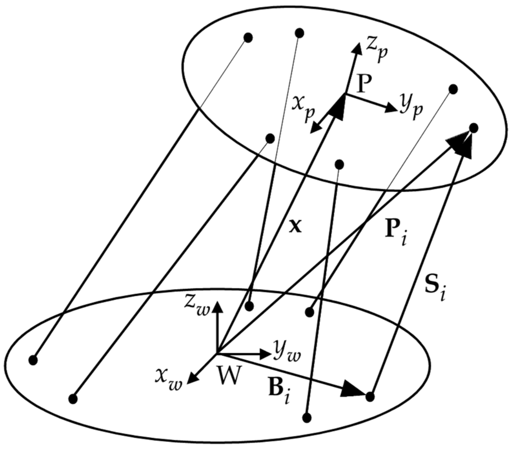
4. Kinematic Model of the Stewart Platform

The Stewart platform, also known as the Gough–Stewart platform, has been selected as a case study since it is the probably the best-known parallel robot. From its introduction in 1956 by Gough as a tire testing machine and in 1965 by Stewart as an aircraft simulation machine, it has attracted considerable research interest in manufacturing and robotic applications. Several commercial machine tools based on this architecture have been proposed. Other application fields are animatronics, crane technology, positioning of satellite dishes, telescopes and surgery devices. Moreover, the Stewart platform is six-degree-of-freedom and non-redundant, which is necessary to apply KDHDc impedance control using Equations (7), (13) and (16). The Stewart platform and its kinematics [25] have been exhaustively discussed and investigated in the scientific literature. In this Section, its geometry and the formulation of the Jacobian matrix, which is used in impedance algorithms, are briefly recalled.
The geometric scheme of a generic Stewart platform is represented in Figure 1. The base is fixed with respect to the fixed reference frame W. The reference frame P is fixed to the moving platform. The external coordinates are composed of the vector x, from the origin of W to the origin of P, and of the angle-axis vector E, which represents the orientation of P with respect to W. The internal coordinates of the robot are the lengths of the six variable-length legs, collected in the vector q. The legs are connected to the base and to the platform by universal joints, and the two parts of each extensible leg are connected by a cylindrical joint with idle rotation and actuated translation. The positions of the centers of the platform and base joints are respectively represented in the frame W by the vectors Pi and Bi.
Let Si be the ith leg vector in the base coordinate system, that is the difference between the position vectors Pi and Bi; the vector Ui of the six Plücker coordinates of the ith leg is composed of the vector Si, normalized and expressed in the platform frame P, and by its moment about the platform reference frame origin, always expressed in frame P:
U i = [ R W P S i | S i | R W P [ ( B i x ) × S i | S i | ] ] .
The static behavior of the Stewart Platform is described by the 6 × 6 matrix U(q), a function of the internal coordinates, which collects the six vectors of the Plücker coordinates [26]:
τ = ( U ( q ) ) 1 F = [ U 1 ( q ) U 2 ( q ) U 3 ( q ) U 4 ( q ) U 5 ( q ) U 6 ( q ) ] 1 F ,
where τ is the vector of the forces exerted by the six legs and F is the six-dimensional vector of the generalized forces exerted by the robot on the environment, expressed on the platform reference frame. Consequently, it is evident that the transpose of U corresponds to the robot Jacobian matrix Jp and can be used in impedance control algorithms (7), (13) and (16). In order to work properly, the Stewart platform should avoid configurations in which the Jacobian matrix is singular or ill-conditioned; to obtain this, first of all the hexagons of the platform and base joints are never regular; moreover, it is convenient to place the joints of platform and base as close as possible two by two, giving rise to two hexagons similar to equilateral triangles, which are rotated 60° in the rest position [27], as in the model shown in Figure 2.

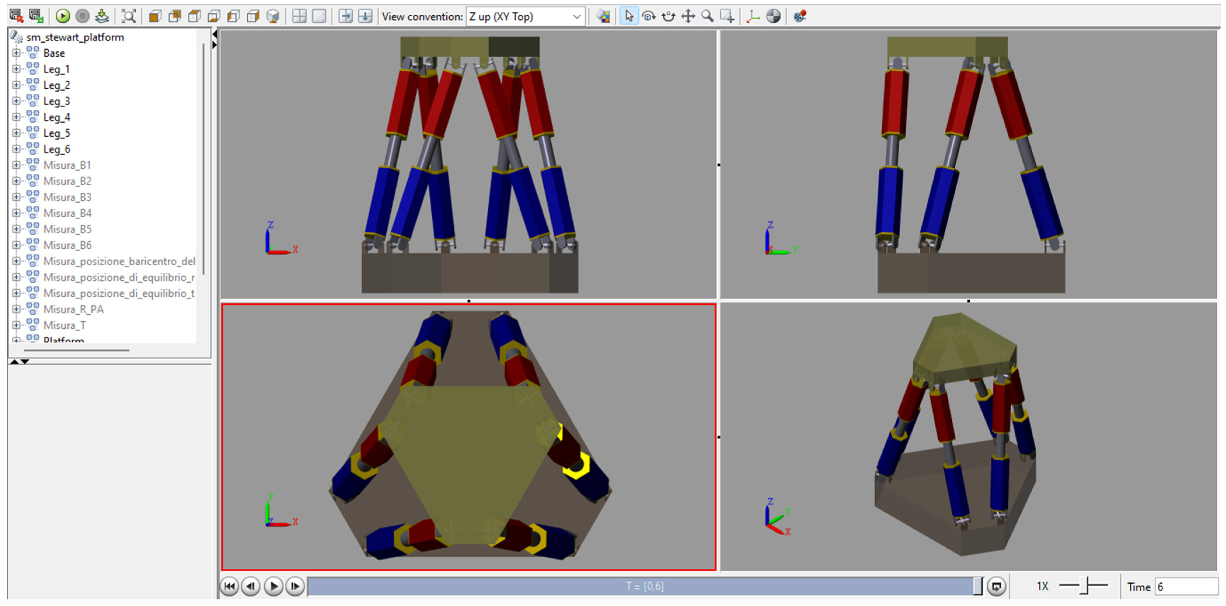
5. Multibody Model of the Stewart Platform

The proposed KDHDc impedance control has been tested and compared to the classical KD control implementing a model of the Stewart platform in the multibody simulation environment Simscape MultibodyTM by MathWorks (Figure 2). The main geometrical and inertial parameters considered in the simulations are collected in Table 1.

6. Simulation Results

The KDHDc/KD comparison has been carried out in a wide variety of case studies; here, for reasons of space, the results of three case studies are reported:
(A)
Approach/depart motion without contact with the environment: the end-effector follows a reference trajectory, defined by time-varying reference values of xd and Ed (external coordinates), without external forces acting on the end-effector; for each external coordinate a trapezoidal speed law is imposed, and the end-effector compliance is isotropic: the stiffness and damping matrices are diagonal, with three equal elements for the translational and rotational submatrices.
(B)
Interaction with the environment: the end-effector reference external coordinates are constant, and an external generalized force is applied to the end-effector. The stiffness and damping matrices are diagonal in the world frame W, which coincides with the principal stiffness/damping reference frames PT and PR, but the end-effector behavior is not isotropic, since the three diagonal elements of each submatrix are not equal.
(C)
Interaction with the environment: similarly to case B, the end-effector reference external coordinates are constant, and an external generalized force is applied to the end-effector, but differently from case B the principal stiffness/damping frames PT and PR do not coincide with W; therefore, the stiffness and damping matrices are block-diagonal but not diagonal.

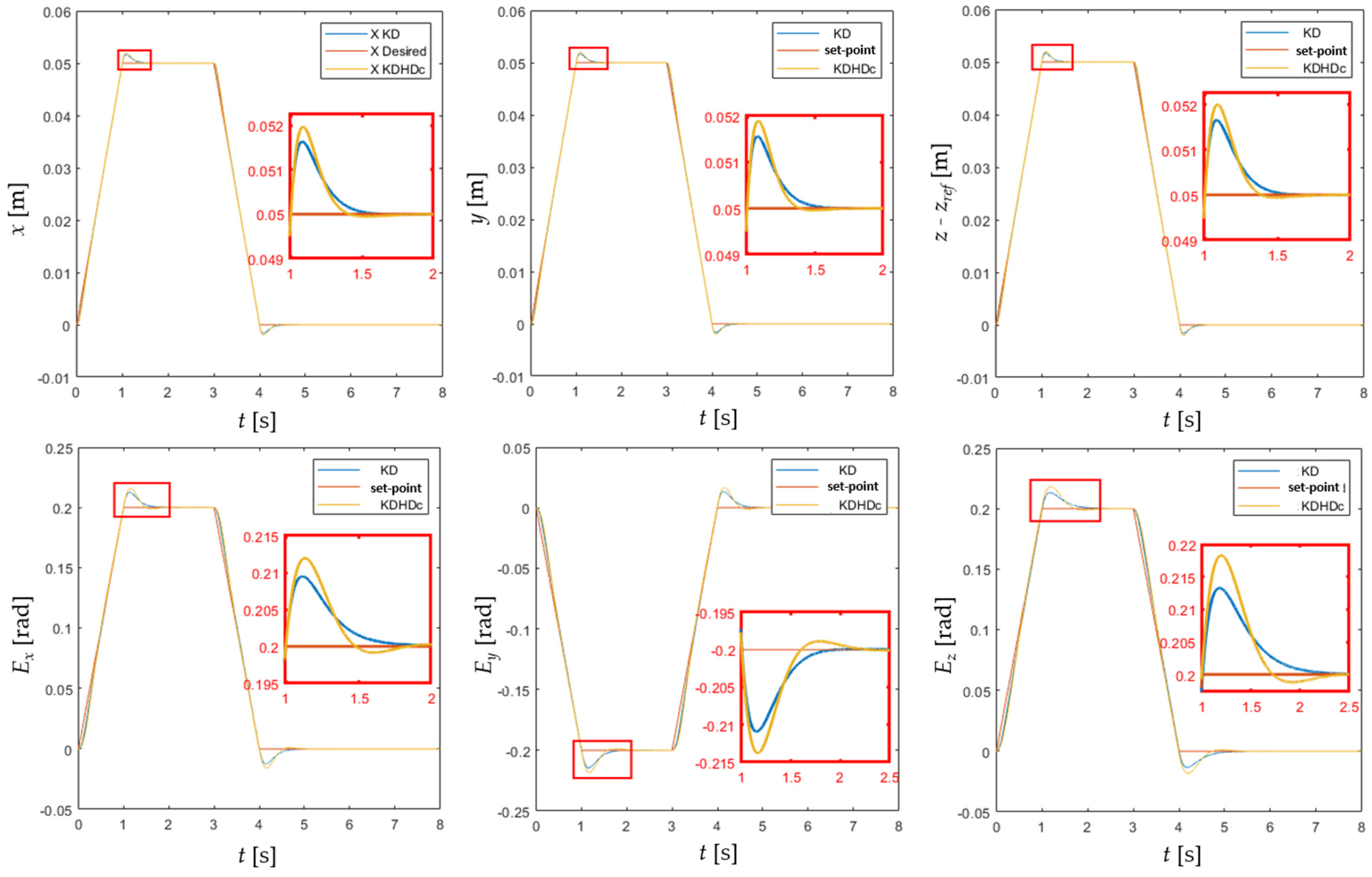
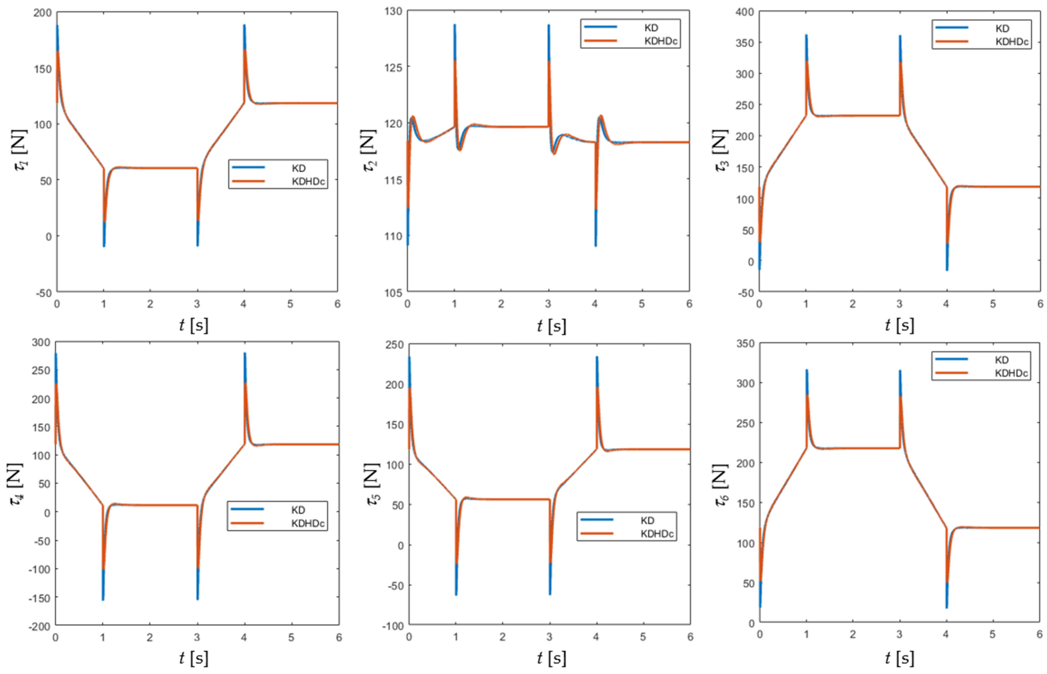
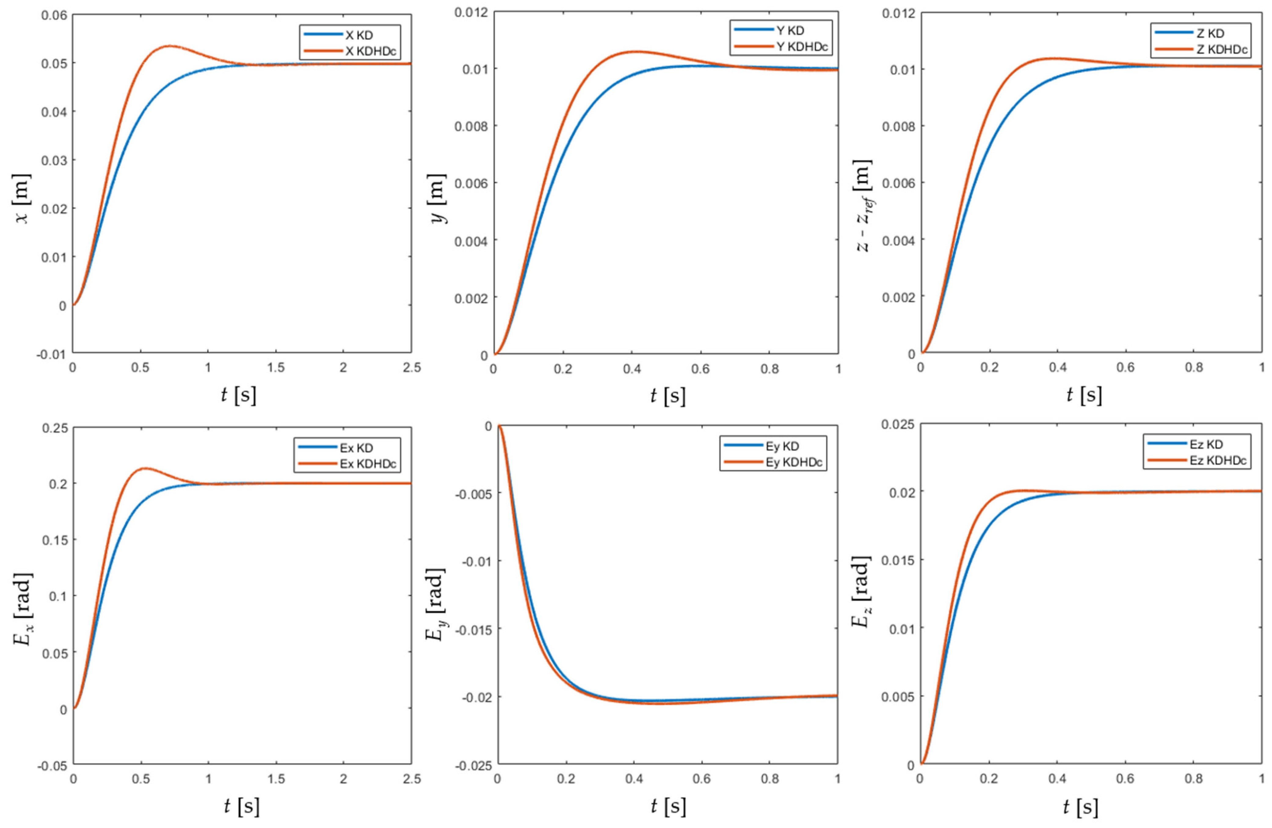
6.1. Case Study A: Approach/Depart Motion without Contact with the Environment

In this case study, the stiffness and damping matrices are diagonal and isotropic both for the KD and KDHD impedance controllers.
For the KD impedance algorithm:
  • KKDt is diagonal with diagonal values kKDt,i, i = 1…3;
  • KKDr is diagonal with diagonal values kKDr,i, i = 1…3;
  • DKDt is diagonal with diagonal values dKDt,i, i = 1…3;
  • DKDr is diagonal with diagonal values dKDr,i, i = 1…3.
After imposing the stiffness diagonal values, the diagonal values of the damping matrix are selected starting from the nondimensional damping coefficient, ζKD, according to the following expression [28]:
d K D t , i = 2 ζ K D t k K D t , i m m p , i = 1 3 ,
d K D r , i = 2 ζ K D r k K D r , i J i , i = 1 3 ,
in which the mass of the moving platform, mmp, is considered for the translational damping, and the three moments of inertia of the moving platform, J1, J2 and J3, are considered for the rotational damping. In general, the nondimensional damping coefficient can have different values for the translational impedance (ζKDt) and for the rotational impedance (ζKDr).
For the KDHDc impedance algorithm:
  • KKDHDt is diagonal with diagonal values kKDHDt,i, i = 1…3;
  • KKDHDr is diagonal with diagonal values kKDHDr,i, i = 1…3;
  • DKDHDt is diagonal with diagonal values dKDHDt,i, i = 1…3;
  • DKDHDr is diagonal with diagonal values dKDHDr,i, i = 1…3;
  • HDKDHDt is diagonal with diagonal values hdKDHDt,i, i = 1…3;
  • HDKDHDr is diagonal with diagonal values hdKDHDr,i, i = 1…3.
The diagonal values of the two damping matrices can be selected starting from the nondimensional coefficients ζKDHD and ψKDHD, according to the following expressions:
d K D H D t , i = 2 ζ K D H D t k K D H D t , i m m p , i = 1 3 ,
d K D H D r , i = 2 ζ K D H D r k K D H D r , i J i , i = 1 3 ,
h d K D H D t , i = ψ K D H D t , i 3 / 4 m m p 1 / 4 , i = 1 3 ,
h d K D H D r , i = ψ K D H D r , i 3 / 4 J i 1 / 4 , i = 1 3 .
The coefficients ζKDHD and ψKDHD represent non-dimensionally the derivative and half-derivative damping terms [28]. In [20], three couples of PD and PDD1/2 tunings, recalled in Table 2, have been compared in the control of a linear axis.
These couples of PD and PDD1/2 tunings have been selected as the starting point of the study, since they have been obtained with reference to a nondimensional second-order purely inertial linear system, with transfer function G(s) = 1/s2, according to the following method:
  • A PD closed-loop control with a given ζ (reference PD) is applied to the position control of G(s), applying a step input, and the settling energy of the step response is calculated.
  • There are infinite combinations of ζ and ψ for a PDD1/2 controller with the same proportional gain and the same settling energy of the reference PD; among these, the ζψ combination which minimizes the settling time is selected.
Table 2 collects the PDD1/2 ζψ combinations associated to three different reference PD controllers, with ζ = 0.8, 1, and 1.2. Simulations and experimental tests on a single mechatronic axis, as reported in [20], show that these PDD1/2 tunings allow to improve the readiness with respect to PD, with a similar control effort. Moreover, even if this tuning is based on the step input, the benefits in terms of control readiness of the PDD1/2 controller have been also demonstrated with different reference inputs [28]. In the following, for reasons of space, only the results for the comparison II (KD with ζKD = 1.0 vs. KDHDc with ζKDHD = 0.45 and ψKDHD = 1.4266) will be reported, the other two comparisons leading to qualitatively similar results.
The stiffness matrices for the KD and KDHDc impedance controls have been obtained imposing the following stiffness values:
  • kKDt,i = kKDHDt,i = 1 × 10³ N/m, i = 1…3,
  • kKDr,i = kKDHDr,i = 1 × 10² Nm/rad, i = 1…3,
While the damping matrices have been calculated using Equations (19) to (24).
In the simulations, the half-derivative is calculated using the digital filter (4) with sampling time Ts = 0.005 s and filter order n = 10; these values are suitable for a real-time digital implementation on a commercial controller.
The two control laws have been compared in case of a trapezoidal reference trajectory, both translational and rotational, characterized by four phases. At the beginning of this trajectory, x = xd = xref (Table 1, the reference position in the workspace center) and E = Ed = 0 (the platform is aligned to the base); then:
  • Phase 1: xd varies with constant velocity from xref to xref + [0.05, 0.05, 0.05]T [m], while Ed varies with constant velocity from 0 to [0.2, −0.2, 0.2]T [rad]. The duration of this phase is tramp = 1 s.
  • Phase 2:xd remains constant in xref + [0.05, 0.05, 0.05]T [m] and Ed remains constant in [0.2, −0.2, 0.2]T [rad] for tstop = 2 s.
  • Phase 3:xd and Ed return to the initial values (xref and 0) with constant velocity in tramp.
  • Phase 4:xd and Ed remain constant in xref and 0 for tstop.
The total simulation time is Tsim = 2(tramp + tstop). Figure 3 and Figure 4 show the simulation results of the KD–KDHDc comparison in terms of external coordinates and actuation forces.
Adopting the KDHDc impedance control, the peaks of actuation forces are lower (average reduction over the six actuators: −13%, Figure 4), and the control effort, calculated according to the following equation,
E t o t = i = 1 6 0 T s i m τ i 2 d t ,
is slightly lower (−0.03%). On the other hand, the settling time to within 0.2% of the steady-state displacement for the KDHDc is slightly lower (−3.7% averaged over the six external coordinates, Figure 3), while the overshoot is higher (maximum overshoot for the translational coordinates: +4.0% for the KDHDc and +3.4% for the KD; maximum overshoot for the rotational coordinates: +9.3% for the KDHDc and +7.4% for the KD). Without discussing in detail the possible advantages of the KDHDc and its possible tuning criteria, it is interesting to observe that this results are qualitatively similar to the ones of the PDD1/2 control scheme compared to the classical PD with same ζ and ψ (better readiness and slightly higher overshoot with lower maximum values of the control inputs [20]). This means that the tuning criteria developed for the PDD1/2 control can provide useful indications for tuning the KDHDc impedance control.

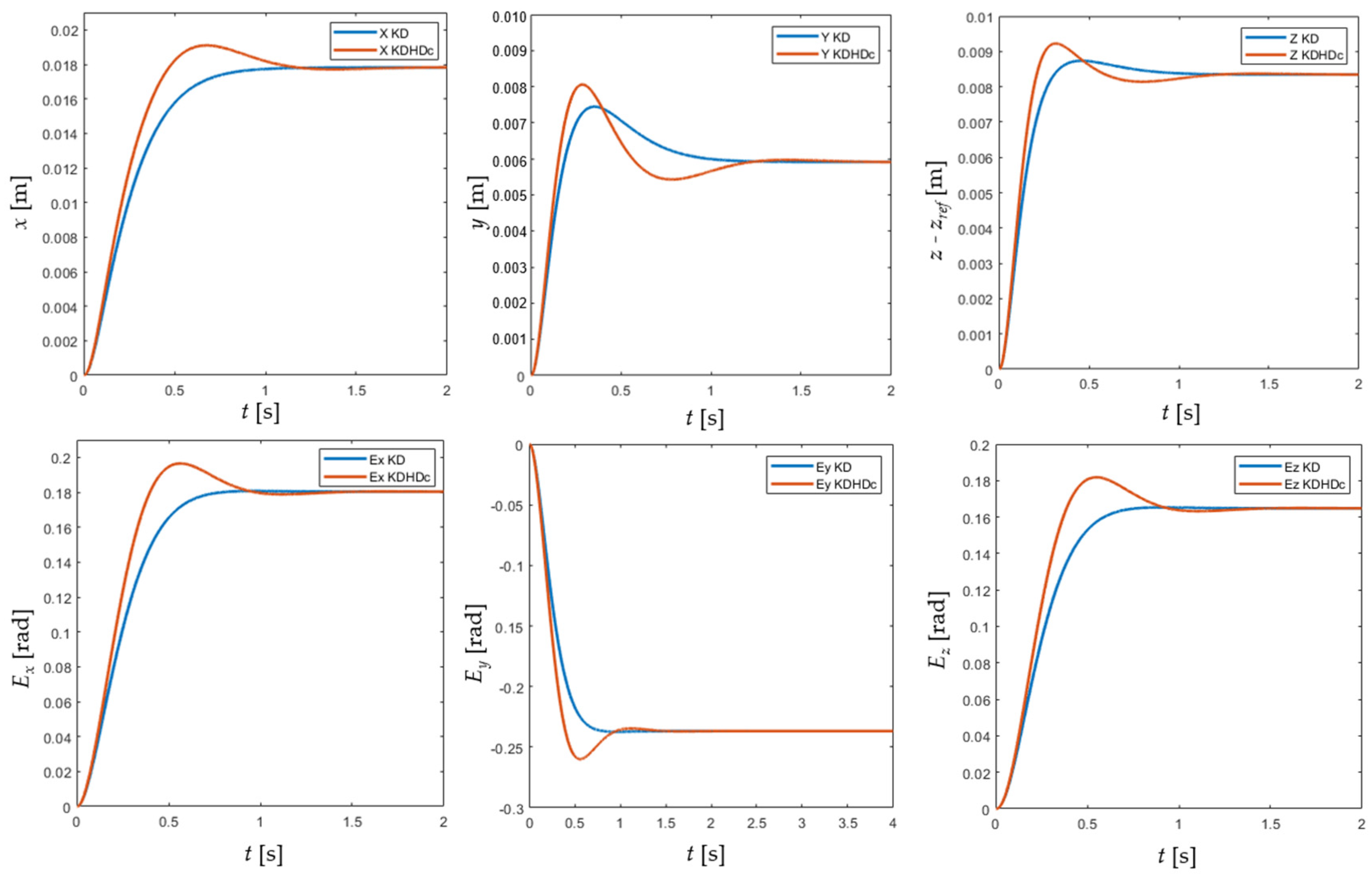
6.2. Case Study B: Interaction with the Environment, Diagonal Stiffness and Damping Matrices

In this case study, the stiffness and damping matrices are diagonal in the world frame W, which coincides with PT and PR, but the imposed end-effector behavior is not isotropic, since the three diagonal elements of each 3 × 3 submatrix are not equal as in case study A:
  • kKDt,1 = kKDHDt,1 = 2 × 10³ N/m; kKDt,2 = kKDHDt,2 = kKDt,3 = kKDHDt,3 = 1 × 10⁴ N/m,
  • kKDr,1 = kKDHDr,1 = 1 × 10² Nm/rad; kKDr,2 = kKDHDr,2 = kKDr,3 = kKDHDr,3 = 1 × 10³ Nm/rad,
Resulting in higher compliance along the x-axis both for the translations and for the rotations. As in case A, the diagonal values of the damping matrices are obtained using Equations (19) to (24) separately for each coordinate, and imposing KD with ζ = 1.0 for the KD, and ζ = 0.45 and ψ = 1.4266 for the KDHDc.
A force F = [100, 100, 100]T N and a moment M = [20, −20, 20]T Nm are applied to the end-effector at t = 0 s. The half-derivative is calculated adopting the same discrete-time implementation as in case A (Ts = 0.005 s, n = 10).
Figure 5 shows the simulation results of the KD–KDHDc comparison in terms of external coordinates. It is possible to note that the steady-state displacements of the external coordinates using the two algorithms coincide for both the algorithms with the expected values, xss and Ess, which can be obtained by inverting the translational and rotational diagonal submatrices:
x s s = ( K K D t ) 1 F = ( K K D H D t ) 1 F = [ 0.05 0.01 0.01 ] T [ mm ] E s s = ( K K D r ) 1 M = ( K K D H D r ) 1 M = [ 0.200 0.020 0.020 ] T [ rad ] .
It occurs thanks to the correctness of the stiffness compensation present in Equation (16) for the KDHDc and absent in Equation (13) for the KDHD; let us note that these correction terms are in percentage relevant with respect to the corresponding diagonal terms of the stiffness matrix: 158%, 105% 105%, 134%, 75% and 89%, respectively, for the six external coordinates. Adopting Equation (13), without this correction, the stiffness of the KDHD is much higher than the desired stiffness expressed by the matrix KKDHD, with diagonal values ranging from 175% to 258% of the corresponding desired values. Let us also note that for the first four external coordinates the negative correction is higher than the desired stiffness, giving rise to negative diagonal values of the proportional terms, without affecting the compensation effectiveness. In other words, the corrected stiffness term of Equation (16) is the sum of two terms, one positive, proportional to the matrix KKDHD of the desired stiffness, and one negative, proportional to the matrix W1/2(n)/Ts1/2HDKDHD. The second negative term, which is the correction of the unwanted additional stiffness introduced by the half-derivative digital filter, depends on the filter order n and on the sampling time Ts, and can be even higher than the desired stiffness term. However, independently of which term is larger, the stiffness compensation acts correctly, and the KDHDc impedance control, Equation (16), exhibits in steady-state the desired stiffness for each external coordinate, as shown by the graphs of Figure 5.

6.3. Case Study C: Interaction with the Environment, Non-Diagonal Stiffness and Damping Matrices

In this case study, the stiffness compensation of the impedance control law KDHDc is tested with the principal translational and rotational reference frames, PT and PR, rotated with respect to the fixed reference frame W: PT is rotated with respect to a W of θt = π/6 rad about an axis represented by the unit vector ut = [+1, −2, +4]T/211/2; PR is rotated with respect to a W of θt = π/3 rad about an axis represented by the unit vector ur = [+1, +2, +4]T/211/2. The rotation matrix between W and PT can be obtained from the axis-angle representation by the following formula [6]:
R W P T = [ u t x 2 + ( 1 u t x 2 ) c θ t u t x u t y ( 1 c θ t ) u t z s θ t u t x u t z ( 1 c θ t ) + u t y s θ t u t x u t y ( 1 c θ t ) + u t z s θ t u t y 2 + ( 1 u t y 2 ) c θ t u t y u t z ( 1 cos θ t ) u t x s θ t u t x u t z ( 1 c θ t ) u t y s θ t u t y u t z ( 1 c θ t ) + u t x s θ t u t z 2 + ( 1 u t z 2 ) c θ t ] .
where cθt and sθt stand for cosθt and sinθt. The rotation matrix between W and PR can be obtained from the same Equation (27), replacing θt and ut with θr and ur.
The principal stiffness matrix and damping matrices have the same diagonal values of case study B, but the stiffness matrix and damping matrices expressed in W change due to the orientations of PT and PR; on the contrary, the external force and moment F and M are kept equal in frame W to case B. The half-derivative is calculated adopting the same discrete-time implementation as in cases A and B (Ts = 0.005 s, n = 10). Figure 6 shows the simulation results in terms of external coordinates for the KD and KDHDc control laws.
It is possible to note that also in this case the steady-state displacements of the external coordinates using the two algorithms coincide for both the algorithms with the expected values, xss and Ess, which can be obtained by inverting the translational and rotational diagonal submatrices, once transformed in the fixed reference frame by Equations (9) and (10), confirming the correctness of the KDHDc stiffness compensation:
x s s = ( K K D t ) 1 F = ( ( R W P T ) T K K D t P T   R W P T ) 1 F = [ 0.0180 0.0059 0.0082 ] T [ mm ] E s s = ( K K D r ) 1 M = ( ( R W P R ) T K K D r P R   R W P R ) 1 M = [ 0.181 0.237 0.165 ] T [ rad ]

7. Conclusions and Future Research Directions

In this paper, the KDHDc fractional-order extension of the classical KD impedance control algorithm, already proposed in [18] for a purely translational parallel robot, has been applied to a six-degree-of-freedom parallel robot, the Stewart platform, requiring the definition of the rotational impedance. To this end, for the representation of the moving platform orientation, which influences the rotational impedance, the three components of the angle-axis vector E have been selected. Using these external coordinates for evaluating the orientation error and its derivatives has some theoretical advantages over other representations (for instance, Euler angles) due to the fact that E is a frame-independent natural invariant with a clear Euclidean-geometric meaning [6], and its first-order derivative has a close relationship with the angular velocity vector, which makes it particularly suitable for defining the damping term [9].
The conception of the KDHDc impedance control originates from the work on the PDD1/2 control scheme, first developed for single-input single-output systems, and can be considered as its extension to impedance-controlled robots, which are a class of non-linear multi-input multi-output systems.
In this paper and in [18] non-redundant parallel robots are considered, but the proposed KDHDc impedance control can be applied also to non-redundant serial robots, only bearing in mind that the Jacobian matrix of serial robots usually transforms the internal coordinates into external coordinates and not vice versa, as for parallel robots. Consequently, the KDHDc impedance control equations proposed in [18] for translational parallel robots and in this paper for full-mobility parallel robots can be used, respectively, for translational and full-mobility serial robots by simply replacing (JT(q))−1 with JT(q).
Even if the work is only a starting point, it is possible to summarize the following conclusions:
  • The application of the half-derivative damping term allows for tuning of the impedance control with additional degrees of freedom, with potential benefits. For instance, the tuning criterion used in case study A, derived from the one proposed in [20] for a single-degree-of-freedom, an almost linear mechatronic axis, leads in free motion to lower actuation forces, almost equal control effort, lower settling time with slightly higher overshoot. These results are qualitatively similar to what happens for the single mechatronic axis, conforming the validity of the approach of deriving the KDHDc tuning form the PDD1/2 tuning. However, the system can be tuned differently, focusing on other performance indices, exploiting the additional regulation opportunities provided by the half-derivative damping.
  • The real-time digital implementation of the half-derivative term introduces a remarkable alteration to the stiffness of the impedance control in steady state, as discussed in Section 2, invalidating the capability of the KDHD impedance control to regulate the contact force between the end-effector and the environment through the measurement of the position error. Nevertheless, the proposed KDHDc compensation, Equation (16), has been proven to be effective also for the rotational behavior (case studies B and C).
Some of the possible future research directions are the following:
  • a systematic investigation on possible tuning approaches for the KDHDc impedance control will be carried out, in order to maximize different performance indices; to this aim, both extension of PDD1/2 tuning methods and numerical optimization techniques will be considered;
  • the KDHDc impedance control will be applied to different serial and parallel architectures; by now, two kinds of mobilities have been taken into account: three translational degrees of freedom and full mobility, without redundancy (equal numbers of internal and external coordinates); in the following, also the cases of limited-degree-of-freedom robots, mixing translational and rotational motions, will be analyzed, both for serial [29,30] and parallel/hybrid manipulators [31,32];
  • impedance control of redundant manipulators, which has interesting theoretical aspects [33], will also be considered;
  • the problem of impedance control for manipulators equipped with flexure joints [34], requiring a proper stiffness compensation of the joint elastic return force, should be addressed;
  • another possible application of the proposed fractional-order approach is impedance control of cable-driven parallel robots [35];
  • as regards the validation methodology, only simulation results are available by now; in the future, besides performing experimental tests of the considered case studies (approach/depart motions without external forces, interactions with the environment with constant force/moment) the effectiveness of the KDHDc impedance control will be assessed in real working conditions, for example peg-in-hole or milling tasks.

Author Contributions

L.B. conceived the control algorithm and designed the simulation campaign; A.P. developed the multibody model and performed simulations; L.B. and A.P. prepared the manuscript. All authors have read and agreed to the published version of the manuscript.

Funding

This research received no external funding.

Institutional Review Board Statement

Not applicable.

Informed Consent Statement

Not applicable.

Data Availability Statement

Data is contained within the article. The simulation data presented in this study are available in figures and tables.

Conflicts of Interest

The authors declare no conflict of interest.

References

  1. Craig, J. Introduction to Robotics. Mechanics and Control; Addison-Wesley: Boston, MA, USA, 1989. [Google Scholar]
  2. Raibert, M.H.; Craig, J.J. Hybrid Position/Force Control of Manipulators. ASME J. Dyn. Syst. Meas. Control 1981, 103, 126–133. [Google Scholar] [CrossRef]
  3. Caccavale, F.; Siciliano, B.; Villani, L. Robot Impedance Control with Nondiagonal Stiffness. IEEE Trans. Autom. Control 1999, 44, 1943–1946. [Google Scholar] [CrossRef]
  4. Valency, T.; Zacksenhouse, M. Accuracy/Robustness Dilemma in Impedance Control. J. Dyn. Syst. Meas. Control 2003, 125, 310–319. [Google Scholar] [CrossRef]
  5. Bruzzone, L.; Molfino, R.M.; Zoppi, M. An impedance-controlled parallel robot for high-speed assembly of white goods. Ind. Robot Int. J. 2005, 32, 226–233. [Google Scholar] [CrossRef]
  6. Angeles, J. Rational Kinematics; Springer: New York, NY, USA, 1988. [Google Scholar]
  7. Bonev, I.A.; Ryu, J. A new approach to orientation workspace analysis of 6-DOF parallel manipulators. Mech. Mach. Theory 2001, 36, 15–28. [Google Scholar] [CrossRef]
  8. Caccavale, F.; Siciliano, B.; Villani, L. The role of Euler parameters in robot control. Asian J. Control 1999, 1, 25–34. [Google Scholar] [CrossRef]
  9. Bruzzone, L.; Molfino, R.M. A geometric definition of rotational stiffness and damping applied to impedance control of parallel robots. Int. J. Robot. Autom. 2006, 21, 197–205. [Google Scholar] [CrossRef]
  10. Ikeura, R.; Inooka, H. Variable impedance control of a robot for cooperation with a human. In Proceedings of the 1995 IEEE International Conference on Robotics and Automation, Nagoya, Japan, 21–27 May 1995; Volume 3, pp. 3097–3102. [Google Scholar]
  11. Tsumugiwa, T.; Yokogawa, R.; Hara, K. Variable impedance control with virtual stiffness for human-robot cooperative peg-in-hole task. In Proceedings of the IEEE/RSJ International Conference on Intelligent Robots and Systems, Lausanne, Switzerland, 30 September–4 October 2002; Volume 2, pp. 1075–1081. [Google Scholar]
  12. Shimizu, M. Nonlinear impedance control to maintain robot position within specified ranges. In Proceedings of the 2012 SICE Annual Conference (SICE), Akita, Japan, 20–23 August 2012; pp. 1287–1292. [Google Scholar]
  13. Miller, K.S.; Ross, B. An Introduction to the Fractional Calculus and Fractional Differential Equations; John Wiley & Sons: New York, NY, USA, 1993. [Google Scholar]
  14. Kizir, S.; Elşavi, A. Position-Based Fractional-Order Impedance Control of a 2 DOF Serial Manipulator. Robotica 2021, 39, 1560–1574. [Google Scholar] [CrossRef]
  15. Liu, X.; Wang, S.; Luo, Y. Fractional-order impedance control design for robot manipulator. In Proceedings of the ASME 2021 International Design Engineering Technical Conferences and Computers and Information in Engineering Conference, Virtual, Online, 17–19 August 2021; Volume 7, p. V007T07A028. [Google Scholar]
  16. Fotuhi, M.J.; Bingul, Z. Novel fractional hybrid impedance control of series elastic muscle-tendon actuator. Ind. Robot Int. J. Robot. Res. Appl. 2021, 48, 532–543. [Google Scholar] [CrossRef]
  17. Podlubny, I. Fractional-order systems and PIλDμ controllers. IEEE Trans. Autom. Control 1999, 44, 208–213. [Google Scholar] [CrossRef]
  18. Bruzzone, L.; Fanghella, P.; Basso, D. Application of the Half-Order Derivative to Impedance Control of the 3-PUU Parallel Robot. Actuators 2022, 11, 45. [Google Scholar] [CrossRef]
  19. Bruzzone, L.; Fanghella, P. Comparison of PDD1/2 and PDμ position controls of a second order linear system. In Proceedings of the IASTED International Conference on Modelling, Identification and Control, Innsbruck, Austria, 17–19 February 2014; pp. 182–188. [Google Scholar]
  20. Bruzzone, L.; Fanghella, P. Fractional-order control of a micrometric linear axis. J. Control Sci. Eng. 2013, 2013, 947428. [Google Scholar] [CrossRef] [Green Version]
  21. Bruzzone, L.; Fanghella, P.; Baggetta, M. Experimental assessment of fractional-order PDD1/2 control of a brushless DC motor with inertial load. Actuators 2020, 9, 13. [Google Scholar] [CrossRef] [Green Version]
  22. Machado, J.T. Fractional-order derivative approximations in discrete-time control systems. J. Syst. Anal. Model. Simul. 1999, 34, 419–434. [Google Scholar]
  23. Das, S. Functional Fractional Calculus; Springer: Berlin/Heidelberg, Germany, 2011. [Google Scholar]
  24. Bruzzone, L.; Callegari, M. Application of the rotation matrix natural invariants to impedance control of rotational parallel robots. Adv. Mech. Eng. 2010, 2010, 284976. [Google Scholar] [CrossRef]
  25. Stewart, D. A Platform with Six Degrees of Freedom. Proc. Inst. Mech. Eng. 1965, 180, 371–386. [Google Scholar] [CrossRef]
  26. Fichter, E.F. A Stewart Platform-based Manipulator: General Theory and Practical Construction. Int. J. Robot. Res. 1986, 5, 157–182. [Google Scholar] [CrossRef]
  27. Ma, O.; Angeles, J. Optimum Architecture Design of Platform Manipulators. In Proceedings of the 5th International Conference on Advanced Robotics, Pisa, Italy, 19–22 June 1991; Volume 2, pp. 1130–1135. [Google Scholar]
  28. Bruzzone, L.; Bozzini, G. PDD1/2 control of purely inertial systems: Nondimensional analysis of the ramp response. In Proceedings of the IASTED International Conference on Modelling, Identification and Control, Innsbruck, Austria, 14–16 February 2011; pp. 308–315. [Google Scholar]
  29. Makino, H.; Furuya, N. Selective compliance assembly robot arm. In Proceedings of the First International Conference on Assembly Automation (ICAA), Brighton, UK, 25–27 March 1980; pp. 77–86. [Google Scholar]
  30. Bruzzone, L.; Bozzini, G. A statically balanced SCARA-like industrial manipulator with high energetic efficiency. Meccanica 2011, 46, 771–784. [Google Scholar] [CrossRef]
  31. Fang, Y.; Tsai, L.-W. Structure synthesis of a class of 4-DoF and 5-DoF parallel manipulators with identical limb structures. Int. J. Robot. Res. 2002, 21, 799–810. [Google Scholar] [CrossRef]
  32. Dong, C.; Liu, H.; Xiao, J.; Huang, T. Dynamic Modeling and Design of a 5-DOF Hybrid Robot for Machining. Mech. Mach. Theory 2021, 165, 2021165. [Google Scholar] [CrossRef]
  33. Xiong, G.; Zhou, Y.; Yao, J. Null-Space Impedance Control of 7-Degree-of-Freedom Redundant Manipulators Based on the Arm Angles. Int. J. Adv. Robot. Syst. 2020, 17, 1729881420925297. [Google Scholar] [CrossRef]
  34. Bruzzone, L.; Molfino, R.M. A novel parallel robot for current microassembly applications. Assem. Autom. 2006, 26, 299–306. [Google Scholar] [CrossRef]
  35. Reichert, C.; Müller, K.; Bruckmann, T. Robust Internal Force-Based Impedance Control for Cable-Driven Parallel Robots. Mech. Mach. Sci. 2015, 32, 131–143. [Google Scholar]
Figure 1. Geometric scheme of the Stewart platform; W(xw, yw,zw): fixed reference frame; P(xp, yp,zp): moving platform reference frame.
Machines 10 00604 g001
Figure 2. Multibody model of the Stewart platform.
Machines 10 00604 g002
Figure 3. Case study A, KD–KDHDc comparison, external coordinates.
Machines 10 00604 g003
Figure 4. Case study A, KD–KDHDc comparison, actuation forces.
Machines 10 00604 g004
Figure 5. Case study B, KD–KDHDc comparison, external coordinates.
Machines 10 00604 g005
Figure 6. Case study C, KD–KDHDc comparison, external coordinates.
Machines 10 00604 g006
Table 1. Geometrical and inertial parameters of the 3-PUU parallel robot.
SymbolParameterValueUnit
|Bi|, i = 1…6base platform radius0.28m
|Pix|, i = 1…6moving platform radius0.3864m
angular distances of the platform joint centers20°/100°/20°/100°/20°/100°degrees
angular distances of the base joint centers100°/20°/100°/20°/100°/20°degrees
mmpmoving platform mass, with payload63kg
mlmass of the upper part of one leg1kg
msmass of the lower part of one leg1.5kg
[J1, J2, J3]principal moments of inertia of the moving platform
(frame P)
[1.636, 1.636, 3.221]kg·m2
xref = [0, 0, zref]reference workspace central position[0, 0, 0.69]m
Table 2. Nondimensional parameters of the compared PD and PDD1/2 tunings.
KD/KDHD ComparisonPD Control/
KD Impedance Control
PDD1/2 Control/
KDHD Impedance Control
ζKDζKDHDψKDHD
I0.80.460.7990
II10.451.4266
III1.20.482.1510
Publisher’s Note: MDPI stays neutral with regard to jurisdictional claims in published maps and institutional affiliations.

