Cross-Domain Remaining Useful Life Prediction Based on Adversarial Training

Abstract

Remaining useful life prediction can assess the time to failure of degradation systems. Currently, numerous neural network-based prediction methods have been proposed by researchers. However, most of the work contains an implicit prerequisite: the network training and testing data have the same operating conditions. To solve this problem, an adversarial discriminative domain adaption prediction method based on adversarial training is proposed to improve the accuracy of cross-domain prediction under different working conditions. First, an LSTM feature extraction network is constructed to mine the source domain data and the target domain data for deep feature representation. Subsequently, the parameters of the target domain feature extraction network are adjusted based on the idea of adversarial training to achieve domain invariant feature mining. The proposed scheme is experimented on a publicly available dataset and achieves state-of-the-art prediction performance compared to recent unsupervised domain adaptation prediction methods.

1. Introduction

Remaining useful life (RUL) prediction, an important research component of prognostic and health management (PHM), can estimate the time to failure of complex systems and reduce maintenance costs and risks [1,2,3]. In general, RUL prediction schemes can be divided into two types: physics-based methods and data-driven methods [4].

Physics-based approaches usually use mathematical modeling methods and classical physical models to describe the health state of mechanical systems [5]. Although these methods achieve accurate prediction results and have good interpretability, they require complex domain expertise, which limits the generalizability of these methods [6]. In contrast, data-driven methods, especially neural network methods, are able to directly learn the relationship between monitoring data and RUL labels by designing a rational network structure. A large number of contributing neural network prediction schemes have been proposed and applied, e.g., Convolutional Neural Network (CNN) [7,8,9,10,11], Gated Recurrent Units (GRU) [12,13,14] and Long Short-Term Memory Networks (LSTM) [15,16,17].

However, in terms of data-driven method, it is challenging (intolerably labor-expensive and time-consuming) to collect sufficient run-to-failure data, which may reduce the prediction performance of the prognostic method. Even when enough historical data are available, the pre-trained model under one specific working condition cannot be generalized to another although they are similar [2]. To cope with the aforementioned limitations, models trained under a single operating condition should be adapted to testing data under other operating conditions, i.e., domain adaptation, a sub-problem of transfer learning [18].

In recently RUL prediction schemes, existing domain adaption methods can be mainly grouped into two categories: moment matching methods and adversarial training methods [19,20]. The former methods align feature distributions across domains by minimizing the distribution discrepancy. Zhu et al. [1] proposed transfer multiple layer perceptron (MLP) with Maximum Mean Discrepancy (MMD) loss [21]. The source and target domain training data feed to the MLP at the same time after feature extraction. By reducing the source domain regression loss and MMD loss, the domain-invariant features are obtained. Yu et al. [22] developed a domain adaptive CNN-LSTM (DACL) model with MMD to align the domain distributions and evaluated the model on C-MAPSS dataset. The latter methods achieve cross-domain prediction feature extraction by adversarial training [23]. Da costa et al. [18] proposed an RUL domain adaptation network named LSTM-DANN. Firstly, degraded pattern knowledge is learned in the source domain, and then the source domain regression model is adjusted to adapt to the target domain feature distribution with the gradient inversion layer to achieve cross-domain RUL prediction [24].

In this work, LSTM combined with a domain adaptive scheme of adversarial discriminative learning framework is proposed, LSTM-ADDA. The proposed scheme can search the domain invariant feature space in the training phase using an adversarial training approach [25] to adjust the network parameters of the LSTM extractor to achieve cross-domain RUL prediction. Compared with the latest adversarial method, LSTM-DANN, the proposed method is not required to repeatedly train the source domain regression model to adapt to different target domains. The extraction of cross-domain RUL prediction features is achieved by reversing the domain feature labels. The implementation process is relatively simple and converges faster. To verify the effectiveness of the proposed method, we conduct experiments on the C-MAPSS datasets and compare the RUL prediction results of aircraft engines with LSTM-DANN and other adaptation methods.

The contributions can be summarized as follows:

• A novel unsupervised adversarial learning RUL prediction scheme is proposed, which can adapt to different fault modes and operating settings domain data.
• Our experimental results show that the proposed LSTM-ADDA method achieves competitive performance compared with other unsupervised domain adaptation methods.

In Section 2, LSTM and unsupervised domain adaption methods are reviewed. In Section 3, the proposed LSTM-ADDA architecture and training process are detailed introduced. In Section 4, we briefly describe the dataset preprocess method and list the hyperparameter selection in experiments. In Section 5, the superiority of the proposed method is proved through two sets of comparative experimental results. The conclusion and future research are drawn in Section 6.

2. Background

In this section, we review the problem definition and generalized adversarial learning framework. Subsequently, the adversarial discriminative domain adaptation (ADDA) method and the detailed LSTM structure are introduced.

2.1. Problem Definition

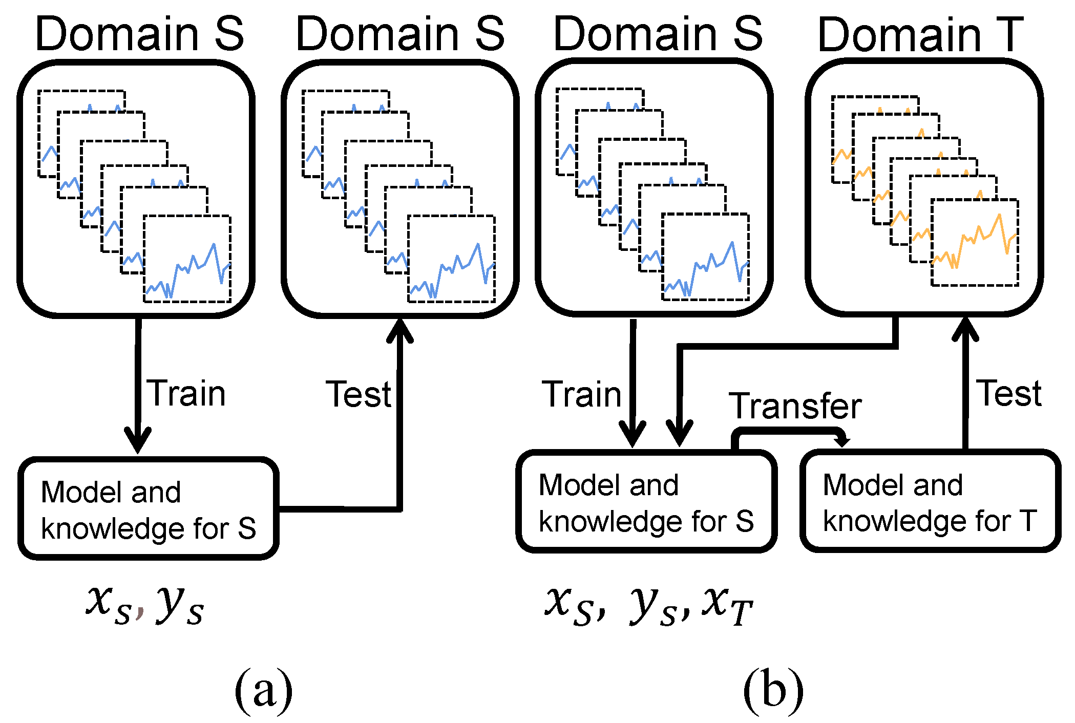
In previous neural network-based prediction methods, training and testing data are usually acquired under the same operating conditions, as shown in Figure 1a. However, it is difficult to obtain data under the same operating conditions in the actual data acquisition, resulting in the limitation of the method’s generalizability. Suppose there are two datasets for remaining useful life prediction under different operating conditions, one of which has sufficient training and testing data (source domain dataset), and the other has only unlabeled training and testing data (target domain dataset). We define this application scenario as an unsupervised domain adaption scenario [26], i.e., with labeled source domain training data and unlabeled target domain training data to predict the target testing data RUL. This paper aims to adaptively implement the prediction of the target domain testing data by transferring the knowledge of the source domain regression model, as shown in Figure 1b. Suppose the source domain data is denoted as $D_S={\left\{(x_S^i,y_S^i)\right\}}_{i=1}^{N_S}$, containing $N_S$ training samples, where $x_S^i$ is a subset of source domain feature space ${\chi }_S$. $T_i$ denotes the length of time and $f_S$ denotes the feature dimensions, i.e., $x_S^i={\left\{x_t^i\right\}}_{t=1}^{T_i}\in {\Re }^{T_i\times f_S}$. Moreover, $y_S^i={\left\{y_t^i\right\}}_{t=1}^{T_i}\in {\Re }_{\ge 0}^{T_i\times 1}$ represents the RUL vector of $x_S^i$. $x_t^i\in {\Re }^{1\times f_S}$ and $y_t^i\in {\Re }_{\ge 0}^1$ denotes the observed feature vector and RUL labels at time $t_i$, respectively. Besides this, we assume a target domain $D_T={\left\{x_T^i\right\}}_{i=1}^{N_T}$, where $x_T^i\in {\chi }_T$ and $x_T^i={\left\{x_t^i\right\}}_{t=1}^{T_i}\in {\Re }^{T_i\times f_T}$. Specially, there are no available RUL labels.

We assume that there are somewhat similar or invariant parts between the deep feature representation of source and target domain mapping. In the model training stage, source domain data and RUL value are available, i.e., ${\left\{(x_S^i,y_S^i)\right\}}_{i=1}^{N_S}$. The target domain data can only use the training monitoring data without RUL labels, ${\left\{x_T^i\right\}}_{i=1}^{N_T}$. It is aimed to adjust the domain feature extractation network g by both source and target training data to perform the target testing sample RUL transfer regression, i.e $y_{true}^i\approx y_{predict}^i=g\left(x_T^i\right)$.

2.2. Generalized Adversarial Adaptation

Tzeng et al. [25] presented a general adversarial adaptive framework, and pointed out that unsupervised domain adaptation could be achieved by reducing the source domain classification loss and alternately minimizing the domain discriminator loss and the distribution discrepancy between the source and target mapping distributions.

Adversarial adaptive methods aim to minimize the distance between the source and target mapping distributions by regularizing the learning of the source and target mappings, $M_S$ and $M_T$. Once the adversarial training is finished, the domain-invariant feature representations are found. Source classification block network can directly receive the target domain feature representation for subsequent RUL prediction, $C=C_S=C_T$.

The source supervised classification network optimize object function is shown as follows:

$$\underset{M_S,C}{min}{\mathcal{L}}_{cls}(x_S^i,y_S^i)=-\sum _{k=1}^K\mathbb{1}(k=y_S^i)logC\left(M_S\left(x_S^i\right)\right)$$

(1)

In adversarial adaptation training part, the domain discriminator, D, is used to distinguishing the source of deep domain features. Similarly, the network parameters of the feature extractor are optimized using the common classification loss, ${\mathcal{L}}_{ad{v}_D}(x_S^i,x_T^i,M_S,M_T)$.

$$\begin{array}{cc}\hfill \underset{D}{min}{\mathcal{L}}_{ad{v}_D}(x_S^i& ,x_T^i,M_S,M_T)=\hfill \\ \hfill -\mathbb{E}& {}_{x_S^i\sim {\chi }_S}\left[logD\left(M_S\left(x_S^i\right)\right)\right]\hfill \\ \hfill -& {\mathbb{E}}_{x_T^i\sim {\chi }_T}\left[log(1-D\left(M_T\left(x_T^i\right)\right))\right]\hfill \end{array}$$

(2)

Finally, the label of the target domain feature representation is reversed to adjust the weights of the target domain mapping structure, achieving the source domain degradation knowledge transfer. The reversed label training loss is denoted as follows, ${\mathcal{L}}_{ad{v}_M}(x_S^i,x_T^i,D)$:

$$\begin{array}{c}\hfill \underset{M_T}{min}{\mathcal{L}}_{ad{v}_M}(x_S^i,x_T^i,D)=-{\mathbb{E}}_{x_T^i\sim {\chi }_T}\left[logD\left(M_T\left(x_T^i\right)\right)\right]\end{array}$$

(3)

2.3. Adversarial Discriminative Domain Adaptation

Adversarial discriminative domain adaptation (ADDA), based on general adversarial adaptive framework, selects the discriminative base model, untied weights and standard GAN loss.

For the mapping optimization constraints, $M_T$ uses the $M_S$ model architecture and weights pre-trained in the source domain during the $M_T$ initialization. In adversarial training, the $M_S$ model is fixed, and the source and target data are input into the $M_S$ and $M_T$, respectively, to obtain feature representations for domain discriminative and $M_T$ weights adjustment. The asymmetric feature representation obtained by unshared weight mappings makes the learning paradigm more flexible.

In adversarial adaptation training, the optimization process is split into two independent objectives, domain discriminator and target feature mapping, and alternately minimizes their loss functions. The ${\mathcal{L}}_{ad{v}_D}$ of domain discriminator remains unchanged, and the target mapping uses the standard loss function of the inverted labels [23].

Similar to the training method of GAN, the mapping feature of the source domain can be labeled as ‘1’ and the target domain as ‘0’, which are input into the discriminator for domain discrimination. During the adversarial training, the mapping feature label of the target is inverted as ‘1’, and input to the discriminator for adversarial training with an inverting the labels manner [26].

The ADDA method divides the optimization process into two stages. First, the $M_S$ and C are trained using labeled source domain data. After that, the $M_S$ is fixed and the $M_T$ is initialized, and the unlabeled target domain data is used to alternately optimize the ${\mathcal{L}}_{ad{v}_D}$ and ${\mathcal{L}}_{ad{v}_M}$ to adjust the model parameters of the $M_T$.

2.4. Long Short-Term Memory Neural Network

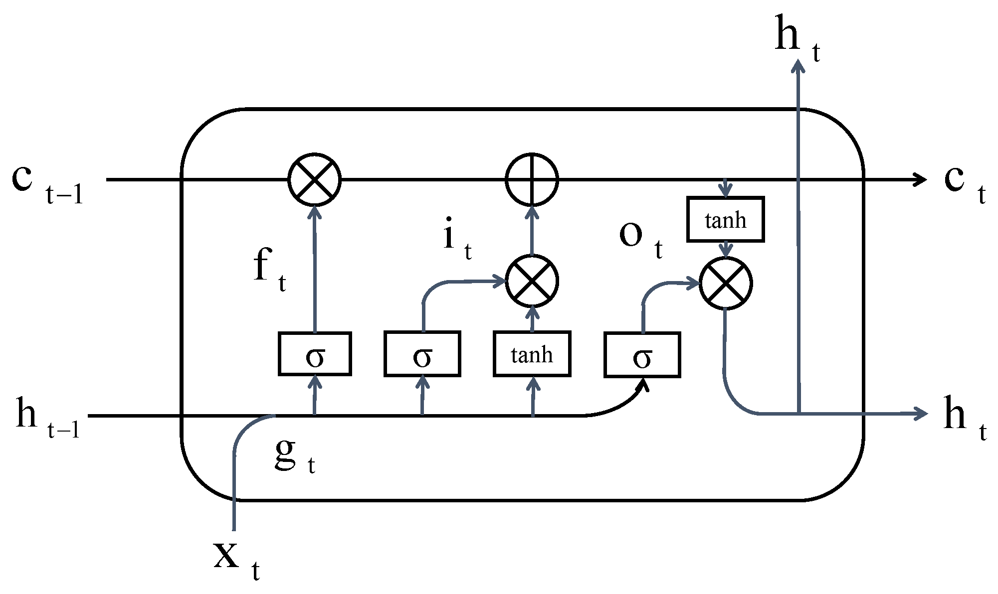
The temporal feature extractor in our methodology is the LSTM network [27], which is a subclass of recurrent neural networks (RNNs). LSTM is one of the most exploited RNN versions because of the capability of detecting long- and short-term dependencies and relaxes the gradient vanishing or exploding problems. As shown in Figure 2, the LSTM cell uses input gate, forget gate and output gate to update current cell state $c_t$ and output hidden state vector $h_t$.

Mathematically, the computation of the LSTM cell can be described as follows:

$$\begin{array}{cc}\hfill & i_t=\sigma (W_{ix}{x}_t+W_{ih}{H}_{t-1}+B_i)\hfill \\ \hfill & g_t=(W_{gx}{x}_t+W_{gh}{H}_{t-1}+B_g)\hfill \\ \hfill & o_t=\sigma (W_{ox}{x}_t+W_{oh}{H}_{t-1}+B_o)\hfill \\ \hfill & c_t=g_t\otimes i_t+c_{t-1}\otimes f_t\hfill \\ \hfill & f_t=\sigma (W_{fx}{x}_t+W_{fh}{H}_{t-1}+B_f)\hfill \\ \hfill & h_t=\left(s_t\right)\otimes o_t\hfill \end{array}$$

(4)

where $W_{gx},W_{ix},W_{fx},W_{ox}$ are weight values between input layer $x_t$ and hidden layer $H_t$ at time t; $W_{gh},W_{ih},W_{fh},W_{oh}$ are hidden layer weight values between time t and $t-1$; $B_g,B_i,B_f,B_o$ are bias of the input layer, input gate, forget gate and output gate, respectively. $H_{t-1}$ is the hidden layer output at previous time. $g_t,i_t,f_t,o_t$ are the output values. $c_t$ represents the current LSTM cell state. ⊗ is the pointwise multiplication operator. $\varphi$, $\sigma$ represent different activation functions.

3. Methodology

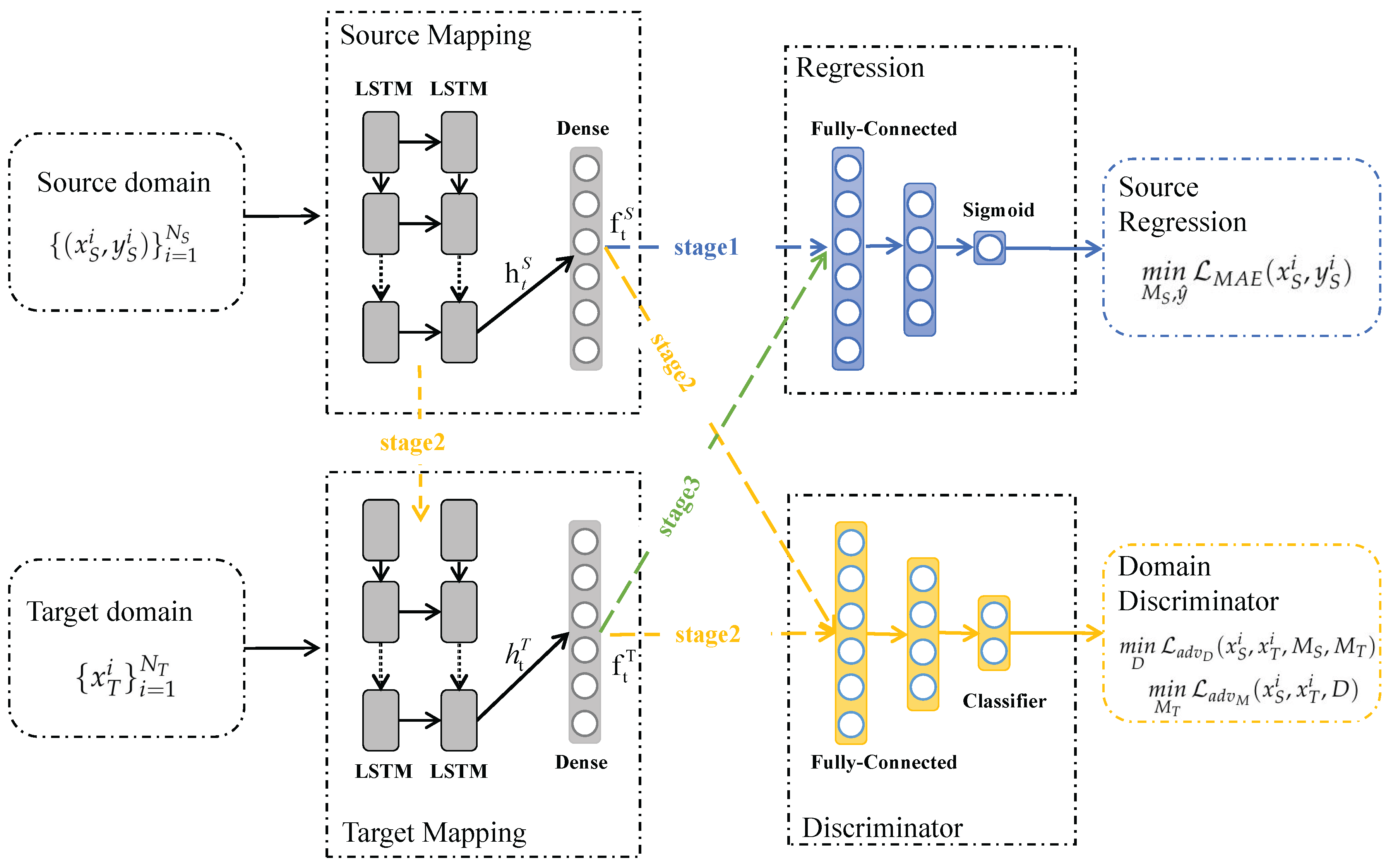
In this section, we detail the proposed method architecture and training processes. Adversarial discriminative domain adaptation based on LSTM, referred as LSTM-ADDA and depicted in Figure 3, can be decomposed into three modules: feature extractor, regression and domain discriminator.

The temporal feature extractor, a combination of LSTMs, establishes a mapping between the input data and the hidden feature state $h_t\in {\Re }^h$. Later, a dense layer transforms the LSTM hidden vector to deep feature representation $f_t\in {\Re }^f$, which will be used as temporal feature space for subsequent regression tasks. The parameters of feature extractor is denoted as ${\Theta }_f$, i.e., $f=g_f(x_S^i;{\Theta }_f).$

Both regression and domain discriminator modules consist of simple fully connected layers. We regard the RUL prediction as a regression task. The mean absolute error (MAE) function is selected as the loss function of the source domain regression to minimization. The parameters in the regression module are denoted as ${\Theta }_{\widehat{y}}$, i.e., $\widehat{y}=g_{\widehat{y}}(g_f(x_S^i;{\Theta }_f);{\Theta }_{\widehat{y}})$. The LSTM-ADDA optimization equations applied in regression scenarios are described as follows:

$$\begin{array}{cc}\hfill \underset{M_S,\widehat{y}}{min}{\mathcal{L}}_{MAE}(& x_S^i,y_S^i)=\left|\widehat{y}-y_S^i\right|=\left|g_{\widehat{y}}(g_f(x_S^i;{\Theta }_f);{\Theta }_{\widehat{y}})-y_S^i\right|\hfill \\ \hfill \underset{D}{min}{\mathcal{L}}_{ad{v}_D}(& x_S^i,x_T^i,M_S,M_T)=-{\mathbb{E}}_{x_S^i\sim {\chi }_S}\left[logD\left(M_S\left(x_S^i\right)\right)\right]-{\mathbb{E}}_{x_T^i\sim {\chi }_T}\left[log(1-D\left(M_T\left(x_T^i\right)\right))\right]\hfill \\ \hfill \underset{M_T}{min}{\mathcal{L}}_{ad{v}_M}(& x_S^i,x_T^i,D)=-{\mathbb{E}}_{x_T^i\sim {\chi }_T}\left[logD\left(M_T\left(x_T^i\right)\right)\right]\hfill \end{array}$$

(5)

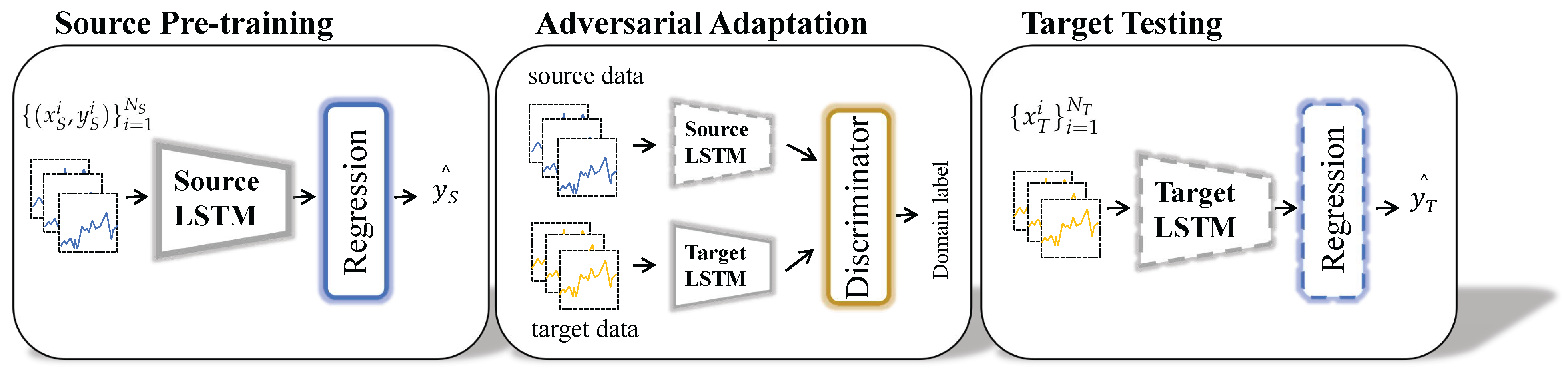
The training process of the proposed method can be summarized into three phases, as shown in Figure 3 and Figure 4.

In stage I, the source domain training data and training labels are input to a source domain regression network consisting of source domain mapping structure and regressor for standard supervised learning training, as shown by the blue arrows in Figure 3. After the source domain training is completed, the network parameters of the source domain mapping structure and regressor will be fixed and will not change with subsequent training. The purpose of stage I is to learn the deep feature representation and degradation patterns of the source domain data from the source domain data.

In stage II, the target domain mapping structure first replicates the structure and parameters of the source domain mapping, which is used as the training starting point for the target domain mapping. Then, the source domain training data and the unlabeled training data of the target domain are input to the source domain mapping and target domain mapping structures to obtain the corresponding deep feature representations, respectively. Subsequently, the feature representations of the two domains are input to the discriminator for adversarial training. The adversarial training is achieved by inverting the domain labels of the two domains. By alternately inverting the domain labels, the parameters of the target domain mapping structure are adjusted to automatically adapt to the data distribution of the target domain, as shown by the orange arrows in Figure 3. Stage II aims to adjust the feature mapping of the target domain to obtain an adaptive target domain deep feature representation for subsequent prediction.

In stage III, the trained target domain mapping structure is combined with the regressor to achieve cross-domain RUL prediction for the target domain testing data, as shown by the green arrows in Figure 3.

For researchers to understand and reproduce the ADDA method, the reference code can be found in the following Github link: https://github.com/acmllearner/pytorch-adda, (accessed on 16 May 2022).

4. Experiment Pre-Settings

In this section, dataset description, data preprocessing, evaluation metric and hyperparameter selection are introduced in this section.

4.1. Dataset Description

The Commercial Modular Aero-Propulsion System Simulation (C-MAPSS) dataset contains four subsets, as shown in

Table 1. The C-MAPSS datasets.

Data Subset	FD001	FD002	FD003	FD004
Training Engine Units (N)	100	260	100	249
Testing Engine Units	100	259	100	248
Operating Conditions (OC)	1	6	1	6
Fault Modes (FM)	1	1	2	2

. Each subset has different fault modes and operating conditions. Each subset contains a training and testing set. Each engine starts with various initial wear but regarded as healthy at the beginning of the recording cycle. Every recording cycle is composed of three operational settings and 21 sensor readings. As the recording cycle increases, each engine performance will gradually degrade until it loses its function [28].

4.2. Data Preprocessing

4.2.1. Time Windows Processing

The sliding time window method is adopted to obtain the same time-window block data. Suppose the running time of an engine $x^i$ is $T_i$, i.e., $x^i={\left\{x_t^i\right\}}_{t=1}^{T_i}$. The sequential input $x^i$ divided by the time window $T_w$ is represented as ${\left\{(x_{t-T_w}^i,\dots ,x_{t-1}^i)\right\}}_{t=T_w+1}^{T_i}$. If $T_i<T_w$, zero-padding is applied to fulfill the ${\mathbf{x}}^i$, i.e., ${\mathbf{x}}^i=\{\stackrel{T_w-T_i}{\overbrace{0,0,\cdots ,0}},$$\underset{T_i}{\underbrace{x_1^i,x_2^i,\cdots ,x_{T_i}^i}}\}.$ This ensures that each engine unit can generate at least two samples. We use the same length of time window to preprocess the source and target domain training sets. To make full use of data, in adversarial training stage, the domain training dataset containing the smaller number of samples is oversampled.

4.2.2. Data Normalization

The min-max normalization is used to scale the subset data (including operating conditions and sensor data) and RUL value to the (0–1) range:

$${\tilde{x}}_t^{i,j}=\frac{x_t^{i,j}-min\left(x^j\right)}{max\left(x^j\right)-min\left(x^j\right)}$$

(6)

where ${\tilde{x}}_t^{i,j}$ denotes the original $ith$ engine unit of the $jth$ feature at record cycle t.

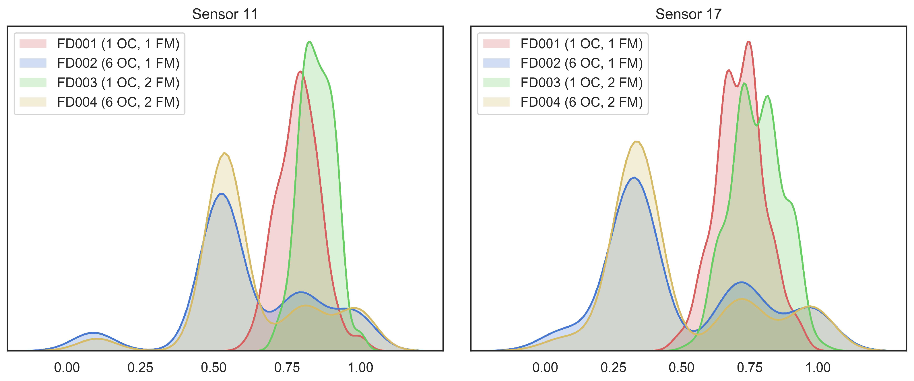
To demonstrate the feature shift between different domains, we perform data distribution statistics on the last cycle of each engine unit in each subset of C-MAPSS. We selected two normalized sensor values for visualization. As shown in Figure 5, we can see that the same operating condition has similar feature distributions for different fault modes. On the contrary, the feature distribution of the same fault mode with the different operating conditions has a clear discrepancy.

As in the previous work [29,30], RUL can be estimated as a constant value in normal operating conditions. Therefore, a piecewise linear degradation model is used to describe the RUL curve of the observation engine. This paper selects $R_e=125$ cycles as the constant RUL before failure and applies it to the training and testing set.

4.3. Performance Metrics

We use two metrics to measure the LSTM-ADDA prognostic performance. The root mean squared error (RMSE), shown in (7), is selected to evaluate the error between the predicted RUL and the actual RUL. We also use the score metric [28], shown in (8), to evaluate our proposed method. The score metric penalizes positive prediction errors more than negative prediction errors because it is more meaningful on maintenance policies to predict failures as early as possible.

$$RMSE=\sqrt{\frac{1}{n}{\sum }_{i=1}^n{(\widehat{RU{L}_i}-ActRU{L}_i)}^2}$$

(7)

$$Score=\left\{\begin{array}{cc}\sum _{i=1}^n{e}^{-\frac{{\widehat{y}}_i-y_i}{13}}-1\hfill & \mathrm{if}{\widehat{y}}_i-y_i<0\hfill \\ \sum _{i=1}^n{e}^{\frac{{\widehat{y}}_i-y_i}{10}}-1\hfill & \mathrm{if}{\widehat{y}}_i-y_i\ge 0\hfill \end{array}\right.$$

(8)

4.4. Hyperparameter Selection

To obtain better adversarial learning performance, we minimize the regression loss in source domain. The learning rate of Adam optimizer is set as 0.0001 (${\lambda }_S$). Besides this, in the adversarial learning process, we reduce the domain classification accuracy of the domain discriminator, i.e., find the domain-invariant representation. For a fair comparison with the adversarial learning method LSTM-DANN [18], we select the same network parameters as the LSTM-DANN method, as shown in

Table 2. Hyperparameter settings for each group of cross-domain prediction.

Source	Target	LSTM Layers,	f	Regression Layers,	Discriminator Layers,	Batch	Optimizer,${\mathit{\lambda }}_{\mathit{T}}$,${\mathit{\lambda }}_{\mathit{D}}$
Domain	Domain	(Units),(Dropout)	(Units)	(Units),(Dropout)	(Units),(Dropout)	Size
FD001	FD002	1,(128),0.5	(64)	1,(32),0.3	1,(32),0.3	256	SGD,0.0001,0.0001
FD001	FD003	1,(128),0.5	(64)	1,(32),0.3	1,(32),0.3	256	SGD,0.0001,0.0001
FD001	FD004	1,(128),0.7	(64)	2,(32,32),0.3	1,(32),0.3	256	SGD,0.0001,0.0001
FD002	FD001	1,(64),0.1	(64)	1,(32),0.0	2,(16,16),0.1	512	SGD,0.0001,0.0001
FD002	FD003	1,(64),0.1	(512)	2,(64,32),0.0	2,(64,32),0.1	256	Adam,0.01,0.01
FD002	FD004	2,(32,32),0.1	(32)	1,(32),0.0	1,(16),0.1	256	SGD,0.0001,0.0001
FD003	FD001	2,(64,32),0.3	(128)	2,(32,32),0.1	2,(32,32),0.1	256	SGD,0.1,0.1
FD003	FD002	2,(64,32),0.3	(64)	2,(32,32),0.1	2,(32,32),0.1	256	Adam,0.1,0.1
FD003	FD004	2,(64,32),0.3	(64)	2,(32,32),0.1	2,(32,32),0.1	256	Adam,0.1,0.1
FD004	FD001	1,(100),0.5	(30)	1,(20),0.0	1,(20),0.1	512	SGD,0.0001,0.0001
FD004	FD002	1,(100),0.5	(30)	1,(20),0.0	1,(20),0.1	512	SGD,0.0001,0.0001
FD004	FD003	1,(100),0.5	(30)	1,(20),0.0	1,(20),0.1	512	SGD,0.0001,0.0001

.

5. Experimental Results

In this section, two comparative experiments are conducted to illustrate the prognostic performance of the proposed method. First, the comparison with the non-adapted models proves that the proposed method can effectively improve the engine RUL prediction under different operating conditions and fault modes. Besides this, compared with other unsupervised transfer learning methods: CORrelation (CORAL) [31], Transfer Component Analysis (TCA) [32] and LSTM-DANN [18].

In the experiment, each training subset of the C-MAPSS dataset is regarded as the source data, and the remaining testing data are regarded as the target data. Therefore, 12 different experiments were performed, and the mean and stand deviations of each experiment result were recorded. All experiments are performed on an Intel Core i7 8th generation processor with 24GB RAM and CPU. We implement our method by using Python 3.6 and Pytorch 1.4.0.

5.1. Non-Adapted Models under Domain Shift

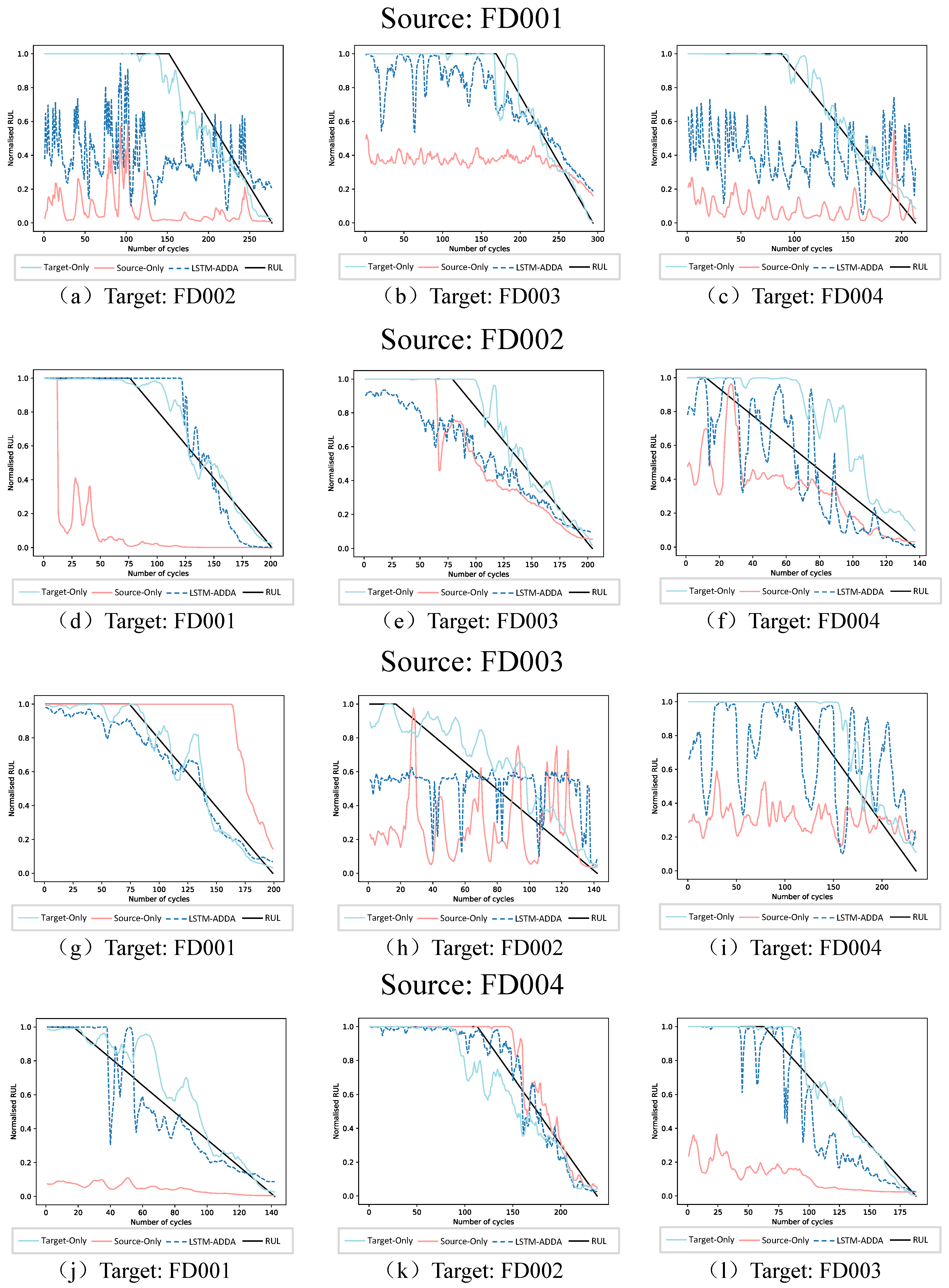
To prove the effectiveness of the proposed adversarial adaption method, we input the target testing data into the source domain model trained on the source domain training data as an experiment of the non-adapted method (source-only). Moreover, we input the target testing data into the target model trained with target domain training data, which represents the ideal situation when the target domain has sufficient training data (target-only). We use each subset of C-MAPSS as the source domain to analyze and discuss the experimental results separately. The results of cross-domain prediction experiments are shown in Figure 6.

Source FD001: FD001 has single fault mode and operating condition, so it is difficult to learn the target domain with complex operating conditions and fault modes, causing the RMSE and prediction scores of LSTM-ADDA higher than the other experiment pairs. As shown in Figure 6a,c, the prediction curve of the proposed model is similar to the source-only waveform and is closer to the target-only curve, indicating that the proposed method can improve the adaptability of the non-adapted model. Compared with the target domain FD003, which has a low distribution discrepancy between the two subsets, the prediction curve obtained in Figure 6b is closer at the end stage of the engine.

Source FD002: Compared with FD001, the operating condition of FD002 is six. When the more complex operating condition dataset as the source domain. as shown in Figure 6d, the proposed model gives better prediction results. When the target domains are FD003 and FD004, containing two fault modes, the prediction effect of FD004 with less domain shift is closer to the target-only curve in Figure 6e. Although the operating conditions and fault modes of FD003 are not the same as FD002, the proposed model can also give better prediction results than the non-adapted models.

Source FD003: Under the same operating conditions, FD003 with two fault modes achieved a lower RMSE when performing adversarial training to the target domain FD001 with one fault mode. Besides this, due to the low distribution discrepancy, Figure 6g shows that the prediction curve obtained by the proposed method also fits the RUL curve of the engine. For FD002 and FD004 with six operating conditions, LSTM-ADDA also gives better prediction results than non-adapted models.

Source FD004: FD004 is containing six operating conditions and two fault modes, which is the most complex subset of the C-MAPSS dataset. When training with the remaining target domain datasets, as shown in

Table 3. Score and RMSE comparsion between Source-Only, Target-Only and LSTM-ADDA. ($\Delta$% denotes the percentage of evaluation metric improvement. ± denotes the standard deviation).

Source	Target	Source-Only	LSTM-ADDA	Source-Only	LSTM-ADDA	Target-Only
		Score	Score	RMSE	RMSE(Δ%)	RMSE
FD001	FD002	672,066.60 ± 98,239.28	54,009.20 ± 9943.48	79.63 ± 1.94	49.60(−37.71%) ± 1.77	18.2 ± 0.31
FD001	FD003	30,523.80 ± 6921.48	4209.80 ± 604.88	56.76 ± 2.39	35.95(−36.66%) ± 1.77	15.57 ± 1.09
FD001	FD004	417,110.20 ± 64,229.99	44,055.20 ± 8788.55	75.58 ± 2.29	50.76(−32.84%) ± 2.44	22.5 ± 0.66
FD002	FD001	160,408.40 ± 84,158.79	12,271.80 ± 10,575.78	70.30 ± 10.93	36.71(−47.79%) ± 2.35	16.15 ± 0.19
FD002	FD003	206,608.40 ± 58,285.75	7374.20 ± 1940.64	75.11 ± 5.25	40.03(−46.70%) ± 3.19	15.57 ± 1.09
FD002	FD004	21,064.20 ± 9648.80	19,085.60 ± 7653.34	36.66 ± 4.24	31.68(−13.58%) ± 1.34	22.5 ± 0.66
FD003	FD001	591,873.60 ± 133,669.19	4644.40 ± 2542.30	54.68 ± 1.93	24.96(−54.35%) ± 2.51	16.15 ± 0.19
FD003	FD002	384,836.40 ± 72,675.49	33,100.60 ± 34,567.30	70.49 ± 3.10	44.17(−37.34%) ± 0.69	18.2 ± 0.31
FD003	FD004	400,365.60 ± 45,021.72	25,577.00 ± 14,002.39	71.11 ± 3.26	44.34(−37.64%) ± 1.24	22.5 ± 0.66
FD004	FD001	172,965.00 ± 140,697.91	38,800.40 ± 23,873.15	72.68 ± 14.99	27.72(−61.87%) ± 1.81	16.15 ± 0.19
FD004	FD002	104,305.40 ± 111,864.98	8588.20 ± 4675.55	28.65 ± 3.44	23.01(−19.68%) ± 1.52	18.2 ± 0.31
FD004	FD003	93,694.00 ± 91,901.72	10,711.40 ± 2832.40	59.98 ± 14.55	32.41(−45.96%) ± 1.90	15.57 ± 1.09

, lower RMSE and prediction scores are obtained. In Figure 6j,l, we can observe that the source-only curve has a large deviation from the RUL curve. For FD002 with a low domain shift, as shown in Figure 6k, the proposed method shows a better fit with the RUL curve.

In summary, the percentage changes of average RMSE and scoring performance between the proposed method and the non-adapted case (source-only) are listed in Table 3. It can be seen that all the prediction performances of the proposed LSTM-ADDA are higher than that of the non-adapted models. Although source-only models can get reasonable performance when the domain shift is small, but the proposed method can further improve the effect. Moreover, when the operating conditions and fault modes of the source domain are complex and the target domain is simple, the LSTM-ADDA model can obtain a better prediction effect. That is to say, it is easier to transfer training from complex situations to simple situations, and it is more difficult to learn from simple situations to complex situations.

5.2. Domain Adaptation Methods Comparison

Two different unsupervised domain adaption methods are used to compare with the proposed method in this section, Transfer Component Analysis (TCA) [32] and CORrelation ALignment (CORAL) [33]. Besides this, the average RMSE and Score are compared with the adversarial method LSTM-DANN.

The distribution of the two domains are mapped together to a high-dimensional Reproducing Kernel Hilbert Space (RKHS). In this space, minimize the MMD between the source and target distribution, while retaining their respective internal attributes.

Different from TCA, CORAL aligns the second-order statistics of the source and target distributions by constructing a differentiable loss function that minimizes the difference between the source and target correlations—the CORAL loss [31].

In the LSTM-DANN method, the source domain shares the network weights with the target domain. When predicting a new target domain, the source domain regression model must be repeatedly trained to extract the degradation knowledge in the source domain. Unlike the LSTM-DANN method, the proposed scheme is not required to train the source-domain regression model repeatedly, and the extraction of cross-domain features can be achieved directly by adversarial training in stage II. Moreover, the significant difference between the proposed and DANN schemes is the cross-domain degradation feature training. The LSTM-DANN method uses the gradient inversion layer, while the LSTM-ADDA method uses the reversed feature domain label. The proposed scheme is simpler to implement and converges faster.

The comparison of the evaluation metrics is shown in

Table 4. Score and RMSE comparsion of unsupervised-domain adaption methods. ($\Delta$% denotes the percentage of evaluation metric improvement. ± denotes the standard deviation).

Source	Target	TCA−DNN	CORAL−DNN	LSTM−DANN	LSTM−ADDA	LSTM−DANN	LSTM−ADDA
		RMSE	RMSE	RMSE	RMSE	Score	Score
FD001	FD002	90.0 ± 2.9	77.5 ± 4.6	48.6 ± 6.8	49.60 ± 1.77	93,841 ± 55,493	54,009.2 ± 9943.5
FD001	FD003	116.1 ± 1.0	69.6 ± 5.2	45.9 ± 3.6	35.95 ± 1.77	27,005 ± 12,385	4209.8 ± 604.9
FD001	FD004	113.8 ± 6.9	84.6 ± 7.0	43.8 ± 4.1	50.76 ± 2.44	57,044 ± 60,160	44,055.2 ± 8788.6
FD002	FD001	85.6 ± 5.5	80.9 ± 9.4	28.1 ± 5.0	36.71 ± 2.35	8411 ± 11,855	12,271.8 ± 10,575.8
FD002	FD003	111.5 ± 7.2	79.8 ± 10.1	37.5 ± 1.5	40.03 ± 3.19	17,406 ± 5702	7374.2 ± 1940.6
FD002	FD004	94.4 ± 6.7	43.6 ± 3.6	31.8 ± 1.6	31.68 ± 1.34	66,305 ± 14,723	19,085.6 ± 7653.3
FD003	FD001	90.5 ± 4.6	26.5 ± 1.9	31.7 ± 9.4	24.96 ± 2.51	5113 ± 4865	4644.4 ± 2542.3
FD003	FD002	80.8 ± 4.3	75.6 ± 9.5	44.6 ± 1.2	44.17 ± 0.69	37,297 ± 15,578	33,100.60 ± 34,567.30
FD003	FD004	102.6 ± 3.2	77.2 ± 9.1	47.9 ± 5.8	44.34 ± 1.24	141,117 ± 66,218	25,577.0 ± 14,002.3
FD004	FD001	85.6 ± 5.0	94.0 ± 8.8	31.5 ± 2.4	27.72 ± 1.81	7586 ± 2735	38,800.4 ± 23,873.2
FD004	FD002	80.8 ± 5.8	30.9 ± 1.4	24.9 ± 1.8	23.01 ± 1.52	17,001 ± 12,927	8588.20 ± 4675.55
FD004	FD003	102.9 ± 2.7	68.6 ± 11.2	27.8 ± 2.7	32.41 ± 1.9	5941 ± 1791	10,711.4 ± 2832.4
Average		96.55	67.40	37.01	36.79 (−0.60%)	40,338.92	21,868.98 (−45.79%)

. We can observe that the mean of RMSE metric is close to LSTM-DANN and overall better than the TCA and CORAL models. In addition, we found that the score metric improved by nearly 45%, indicating that the proposed method can achieve better prediction results in a timely manner while maintaining a smaller RMSE metric, which is more in line with the need for advanced prediction in practical maintenance.

6. Conclusions and Future Work

In this paper, a novel domain adaptation RUL prediction scheme is proposed by combining the LSTM network and adversarial discriminative domain adaptation framework (LSTM-ADDA). The prediction effect of the proposed model is verified on the C-MAPSS dataset. The LSTM feature extractor network parameters are adjusted by the target domain training data to find the domain invariant feature representation.

The proposed method uses the source domain data to obtain source domain degradation knowledge. After that, the target domain data without RUL label is combined for adversarial learning. Finally, the target feature extractor adjusted by adversarial training combines with the source domain regression module to implement the target domain RUL adaption prediction.

To illustrate the effectiveness of the LSTM-ADDA method, we perform two comparative experiments. The experimental results show that the prediction result of the proposed method is better than other methods. In future work, we will try to remove the target domain data from the training process, and use a generalized model combined with multi-source data to directly estimate the RUL of the target domain.

References

- Zhu, J.; Chen, N.; Shen, C. A new data-driven transferable remaining useful life prediction approach for bearing under different working conditions. Mech. Syst. Signal Process. 2020, 139, 106602. [Google Scholar] [CrossRef]
- Lei, Y.; Li, N.; Guo, L.; Li, N.; Yan, T.; Lin, J. Machinery health prognostics: A systematic review from data acquisition to rul prediction. Mech. Syst. Signal Process. 2018, 104, 799–834. [Google Scholar] [CrossRef]
- Zhou, T.; Han, T.; Droguett, E. Towards trustworthy machine fault diagnosis: A probabilistic Bayesian deep learning framework. Reliab. Eng. Syst. Saf. 2022, 224, 108525. [Google Scholar] [CrossRef]
- Fan, Y.; Nowaczyk, S.; Rognvaldsson, T. Transfer learning for remaining useful life prediction based on consensus self-organizing models. Reliab. Eng. Syst. Saf. 2020, 203, 107098. [Google Scholar] [CrossRef]
- Li, N.; Lei, Y.; Lin, J.; Ding, S.X. An improved exponential model for predicting remaining useful life of rolling element bearings. IEEE Trans. Ind. Electron. 2015, 62, 7762–7773. [Google Scholar] [CrossRef]
- Cofre-Martel, S.; Droguett, E.L.; Modarres, M. Uncovering the underlying physics of degrading system behavior through a deep neural network framework: The case of remaining useful life prognosis. arXiv 2020, arXiv:2006.09288. [Google Scholar]
- Zhu, J.; Chen, N.; Peng, W. Estimation of bearing remaining useful life based on multiscale convolutional neural network. IEEE Trans. Ind. Electron. 2018, 66, 3208–3216. [Google Scholar] [CrossRef]
- Yang, B.; Liu, R.; Zio, E. Remaining useful life prediction based on a double-convolutional neural network architecture. IEEE Trans. Ind. Electron. 2019, 66, 9521–9530. [Google Scholar] [CrossRef]
- Xu, X.; Wu, Q.; Li, X.; Huang, B. Dilated convolution neural network for remaining useful life prediction. J. Comput. Inf. Sci. Eng. 2020, 20, 021004. [Google Scholar] [CrossRef]
- Peng, W.; Ye, Z.-S.; Chen, N. Bayesian deep-learning-based health prognostics toward prognostics uncertainly. IEEE Trans. Ind. Electron. 2019, 67, 2283–2293. [Google Scholar] [CrossRef]
- Wang, B.; Lei, Y.; Li, N.; Wang, W. Multi-scale convolutional attention network for predicting remaining useful life of machinery. IEEE Trans. Ind. Electron. 2020, 68, 7496–7504. [Google Scholar] [CrossRef]
- Zhao, R.; Wang, D.; Yan, R.; Mao, K.; Shen, F.; Wang, J. Machine health monitoring using local feature-based gated recurrent unit networks. IEEE Trans. Ind. Electron. 2017, 65, 1539–1548. [Google Scholar] [CrossRef]
- Li, X.; Jiang, H.; Xiong, X.; Shao, H. Rolling bearing health prognosis using a modified health index based hierarchical gated recurrent unit network. Mech. Mach. Theory 2019, 133, 229–249. [Google Scholar] [CrossRef]
- Ren, L.; Cheng, X.; Wang, X.; Cui, J.; Zhang, L. Multi-scale dense gate recurrent unit networks for bearing remaining useful life prediction. Future Gener. Comput. Syst. 2019, 94, 601–609. [Google Scholar] [CrossRef]
- Zhang, Y.; Xiong, R.; He, H.; Pecht, M.G. Long short-term memory recurrent neural network for remaining useful life prediction of lithium-ion batteries. IEEE Trans. Veh. Technol. 2018, 67, 5695–5705. [Google Scholar] [CrossRef]
- Wu, Y.; Yuan, M.; Dong, S.; Lin, L.; Liu, Y. Remaining useful life estimation of engineered systems using vanilla lstm neural networks. Neurocomputing 2018, 275, 167–179. [Google Scholar] [CrossRef]
- TV, V.; Malhotra, P.; Vig, L.; Shroff, G. Data-driven prognostics with predictive uncertainty estimation using ensemble of deep ordinal regression models. arXiv 2019, arXiv:1903.09795. [Google Scholar]
- da Costa, P.R.D.O.; Akcay, A.; Zhang, Y.; Kaymak, U. Remaining useful lifetime prediction via deep domain adaptation. Reliab. Syst. Saf. 2020, 195, 106682. [Google Scholar] [CrossRef] [Green Version]
- Han, T.; Liu, C.; Yang, W.; Jiang, D. A novel adversarial learning framework in deep convolutional neural network for intelligent diagnosis of mechanical faults. Knowl.-Based Syst. 2019, 165, 474–487. [Google Scholar] [CrossRef]
- Wang, X.; Long, M.; Wang, J.; Jordan, M.I. Transferable calibration with lower bias and variance in domain adaptation. arXiv 2020, arXiv:2007.08259. [Google Scholar]
- Ghifary, M.; Kleijn, W.B.; Zhang, M. Domain adaptive neural networks for object recognition. In Pacific Rim International Conference on Artificial Intelligence; Springer: Cham, Switzerland, 2014; pp. 898–904. [Google Scholar]
- Yu, S.; Wu, Z.; Zhu, X.; Pecht, M. A domain adaptive convolutional lstm model for prognostic remaining useful life estimation under variant conditions. In Proceedings of the 2019 Prognostics and System Health Management Conference (PHM-Paris), Paris, France, 2–5 May 2019; pp. 130–137. [Google Scholar]
- Goodfellow, I.; Pouget-Abadie, J.; Mirza, M.; Xu, B.; Warde-Farley, D.; Ozair, S.; Courville, A.; Bengio, Y. Generative adversarial nets. In Proceedings of the Neural Information Processing Systems, Cambridge, MA, USA, 8–13 December 2014; MIT Press: Massachusetts, MA, USA, 2014; pp. 2672–2680. [Google Scholar]
- Ganin, Y.; Ustinova, E.; Ajakan, H.; Germain, P.; Larochelle, H.; Laviolette, F.; Marchand, M.; Lempitsky, V. Domain-adversarial training of neural networks. J. Mach. Learn. Res. 2016, 17. [Google Scholar]
- Tzeng, E.; Hoffman, J.; Saenko, K.; Darrell, T. Adversarial discriminative domain adaptation. In Proceedings of the IEEE Conference on Computer Vision and Pattern Recognition, Honolulu, HI, USA, 21–26 July 2017; pp. 7167–7176. [Google Scholar]
- Wilson, G.; Cook, D.J. A survey of unsupervised deep domain adaptation. ACM Trans. Intell. Syst. Technol. (TIST) 2020, 11, 1–46. [Google Scholar] [CrossRef]
- Hochreiter, S.; Schmidhuber, J. Long short-term memory. Neural Comput. 1997, 9, 1735–1780. [Google Scholar] [CrossRef]
- Saxena, A.; Goebel, K.; Simon, D.; Eklund, N. Damage propagation modeling for aircraft engine run-to-failure simulation. In Proceedings of the IEEE International Conference on Prognostics and Health Management, Denver, CO, USA, 6–9 October 2008; pp. 1–9. [Google Scholar]
- Cai, H.; Jia, X.; Feng, J.; Li, W.; Pahren, L.; Lee, J. A similarity based methodology for machine prognostics by using kernel two sample test. ISA Trans. 2020, 103, 112–121. [Google Scholar] [CrossRef]
- Yu, W.; Kim, I.Y.; Mechefske, C. An improved similarity-based prognostic algorithm for rul estimation using an rnn autoencoder scheme. Reliab. Eng. Syst. Saf. 2020, 199, 106926. [Google Scholar] [CrossRef]
- Sun, B.; Saenko, K. Deep coral: Correlation alignment for deep domain adaptation. In European Conference on Computer Vision; Springer: Cham, Switzerland, 2016; pp. 443–450. [Google Scholar]
- Pan, S.J.; Tsang, I.W.; Kwok, J.T.; Yang, Q. Domain adaptation via transfer component analysis. IEEE Trans. Neural Netw. 2010, 22, 199–210. [Google Scholar] [CrossRef] [Green Version]
- Sun, B.; Feng, J.; Saenko, K. Return of frustratingly easy domain adaptation. In Proceedings of the Thirtieth AAAI Conference on Artificial Intelligence, Phoenix, AZ, USA, 12–17 February 2016. [Google Scholar]