1. Introduction
As the middle mechanism between the base and the carrier, the inertial stabilized platform (ISP) can isolate non-ideal interference effectively to realize a high-performance attitude control for the load line of sight (LOS) [
1]. Therefore, it has become a common key piece of equipment in aerial remote sensing systems [
2].
However, there exist multiple disturbances for the ISP system in the working process, including dynamic unbalanced torque, non-ideal angular motion and linear motion interference, coupling torque and friction interference torque, etc. [
3,
4]. These disturbances have non-Gaussian, slow time-varying, unknown frequency amplitude harmonics, norm-bounded and other complex structural characteristics [
5]. The mechanism of the disturbances are so complex that it is hard for the ISP system to realize high-performance control in real applications [
6].
To improve the system control accuracy and anti-disturbance ability in a complex environment, PID, robust control, sliding mode control (SMC), and neural network (NN) control methods have been proposed. PID control methods are often designed for the ISP system for simple structures [
7]. However, the control performance is easily affected by complex environment disturbances. Robust control methods have shown high adaptability for parameter uncertainty in practical applications. Rezaei D. Mahdy [
8] realized a high-performance control for the ISP system based on the robust control and predictive control method. However, the robust control method has corresponding conservative characteristics with the improvement of the system’s robustness. Although the control performance is easily worsened by the chattering phenomenon, the SMC method can deal with nonlinear systems with external disturbances and uncertainty effectively [
9,
10]. With the improvement requirement of the system robustness, the terminal sliding mode control (TSMC) scheme has been developed. A global fast terminal sliding mode control (GFTSMC) is proposed to guarantee the control system to converge to reference states robustly in desired time, which focused more in finite-time stabilization [
11,
12]. At present, GFTSMC has been applied in many fields, such as unmanned aerial vehicle (UAV) control, permanent magnet synchronous motor (PMSM) control, and so on [
13,
14]. After enough training, the NN control method can deal with nonlinear disturbances effectively [
15,
16]. However, it is hard to generate enough sampling data because of the complexity of the working environment. Combined with the SMC method, the adaptive NN control method is constructed without offline training [
17]. However, the control performance is easily affected by the selection of the upper boundary of residual approximation errors.
Considering the system uncertainty, external disturbances and unmodeled dynamics as the lumped disturbance, the extended state observer (ESO) can estimate and eliminate disturbances effectively [
18,
19]. The parameter adjustment of linear ESO (LESO) is simple and convenient; therefore, LESO is widely used in practical engineering. With the LESO, the unstructural uncertainty of the DC motor can be dealt with effectively [
20]. A. H. M. Sayem [
21] proposed a LESO-based model repetitive control (MRC) method for the servo motor, which can compensate for periodic and non-periodic disturbances effectively. Considering the friction effect as external interference, the compound method based on the SMC and a reduced-order LESO is proposed for the friction compensation of omnidirectional mobile robots (OMRs) to realize high performance control [
22]. However, the observation bandwidth of LESO has a great influence on its state estimation performance. The peaking phenomenon will be generated with the increment of bandwidth when the initial state of the system does not match the estimated state [
23]. At the same time, the impact of input delay on the dynamic tracking error will become more and more obvious [
24].
In this paper, in order to improve the ability to suppress various internal and external disturbances, and realize high control performance for the ISP system, a compound control method based on the adaptive linear ESO (ALESO) and the GFTSMC is proposed, which includes the following contributions:
(1) Considering various internal and external disturbances as the lumped disturbance, the ALESO based on the adaptive bandwidth was developed to estimate the unknown lumped disturbance for the ISP system. With the full use of the information of attitude and angular velocity, it can deal with the peaking phenomenon without introducing excessive noise.
(2) The adaptation law based on the GFTSMC for disturbance estimation compensation was developed to compensate for the disturbance estimation error of ALESO, which can improve the disturbance estimation accuracy of ALESO.
(3) The GFTSMC is proposed to handle the ISP system nonlinearity, parameter variations, internal and external coupling, and disturbances. The higher order terminal function in GFTSMC is replaced by the lumped disturbance estimation of the ALESO, which can improve the anti-interference ability of ISP, reduce the chattering problem, and improve the control performance.
The outline of the paper is organized as follows: In
Section 2, the nonlinear dynamic model of the ISP is constructed and disturbances are analyzed. In
Section 3, the compound control method based on the ALESO and the GFTSMC is proposed to promote control performance, and the adaptation law is established. A series of simulations and experiments validate the effectiveness of the proposed control method in
Section 4, followed by the conclusions in
Section 5.
2. The Nonlinear Dynamic Model and Disturbances Analysis of ISP
A two-axis ISP is designed to locate faults of a high voltage line, whose length, width and height are 0.67 m, 0.17 m and 0.55 m. The ISP system is composed of the pitch and yaw gimbals, shown in
Figure 1. The pitch and yaw gimbals are the inner gimbal and outer gimbal of the ISP system, respectively.
To get different faults information for high voltage lines, a long-focus camera and a short-focus camera, infrared camera, ultraviolet camera, and a 3D laser scanner were chosen as loads for the ISP system, which are located in the pitch box. The system is composed of duralumin LC4, with a total weight of 10.3 kg, and the total load weight of loads is 15.6 kg. To get enough torque to realize high-performance control, a large-torque EM-PIM375 motor with a reduction ratio of 1:4.5 was chosen. Moreover, to reject the high-frequency line vibration of vertical direction, four metal dampers with the same stiffness were installed uniformly between the base and the helicopter.
A high-performance position orientation system (POS) was chosen to provide the attitude angle information of the payloads, whose pitch angle and yaw angle measurement errors are less than 0.003° and 0.005°, respectively. Meanwhile, the open-loop optical fiber rate gyro, VG095M, was chosen to provide angular velocity information of the gimbals. Its constant drift is 15°/h. The rotary electric encoder DS-58-32-DF-C was introduced to the gimbals, whose precision is 0.003°. The ISP system was mounted on the bottom of the unmanned helicopter (UH). With the nonideal angle disturbances of UH, the LOS of the optical imaging sensors will deviate planed angles correspondingly. Since the POS is mounted on the same base of the different optical sensors, it can provide the angle information of the LOS of the optical sensors. Based on the measured information of POS, gyros, and encoders, the controller generates corresponding control signals to adjust the pitch and the yaw gimbal. Therefore, the LOS of the optical imaging sensors is adjusted correspondingly to eliminate angle errors to get precise images and video of the high-voltage wires and the electric towers.
As a typical multi-axis and multi-gimbal system, there exists a complex coordinate transformation process. The base plate coordinate axes were fixed to the base plate, and the yaw coordinate axes were fixed to the yaw gimbal. Furthermore, the pitch coordinate axes were fixed to the pitch gimbal.
There is only the yaw angle about between the base plate coordinate and the yaw coordinate. At the same time, only the pitch angle about was used between the yaw coordinate and the pitch coordinate. The and can be measured by two encoders.
In order to explain the subsequent ISP model, define
as the pitch, the yaw, and the base plate coordinate, respectively.
represents the angular velocity of the
coordinate axes with respect to the geographic coordinate axes expressed in the
coordinate axes.
and
represent the transformation matrixes from the base plate coordinate to the yaw coordinate and the yaw coordinate to the pitch coordinate, respectively. Based on the Newton–Euler theory, the dynamic model of the ISP system can be obtained as follows [
25]:
where the dots represent derivatives of a single variable, and the commas represent derivatives of the entire parenthesis.
,
,
and
can be obtained by
,
and the transformation matrices
and
.
and
are the moment of inertia of pitch and yaw gimbal in three directions, respectively.
,
.
is the moment of inertia of the motor.
,
and
are the torque sensitivity, the back EMF constant, and the motor resistance, respectively. The
is the gear ratio of the motor.
and
are the voltage input applied on the pitch and yaw gimbal motor armature, respectively.
and
are the torque disturbances imposed on the pitch and yaw gimbal, respectively, including mass imbalance torque and other unknown disturbances, such as wind disturbance. Moreover,
is the torque disturbance imposed on the motor, which is caused by the residual vibration disturbances generated by the main rotor and the bearing friction, cogging, and imperfections in the motor.
With the analysis of the ISP system, the mass imbalance torque, the gimbal friction torque, the residual vibration disturbances generated by the main rotor, and the non-ideal angular motion interference generated by wind disturbance play important roles in the system errors.
The major part of
is the mass imbalance torque. In the ISP system exists a certain mass imbalance with the diversity of payloads. For real application, the maximum mass imbalance distance is required to be less than
, and the maximum weight of the payloads is often less than
, so the mass imbalance torque is
. Meanwhile, in order to verify the effectiveness of the proposed control method, a certain random torque
was used to simulate the wind disturbance.
is the amplitude of wind disturbance. Therefore,
is represented by the disturbance with certain bounds in the ISP system
Friction torque is the first part of
. The high-performance brushless DC torque motors are proposed to provide enough torque to adjust gimbal angle, where the sliding friction coefficient is
. The weight and the radius of the motor gear are
and
, respectively. Since there exists a certain relationship between the friction torque and the frequency of the motion of the ISP [
17], the
is represented by the superposition of sinusoidal functions
where
is the fundamental frequency of sinusoidal functions.
The second part of
is the residual vibration disturbances. Since the high frequency periodic disturbances whose frequency surpass 10 Hz have been isolated effectively by the metal dampers, the certain sinusoidal torque
was used to simulate the residual periodic vibration disturbances.
is the amplitude of vibration disturbances. Therefore,
is represented by the disturbance within certain bounds in the ISP system
In order to facilitate the design of the controller and for engineering practicality, (1) and (2) can be rewritten as
where
,
,
includes the unmodeled friction, dead zone, hysteresis, and the unknown uncertainties of
,
,
and
,
.
3. The Compound Control Method of the ISP
Since
,
are nonlinear and time-variant functions and contain the internal and external coupling of the gimbals, and there exist measurement errors and unknown disturbances, it is hard to generate suitable control commands to realize high-performance control. To improve the control performance, a compound control method based on the ALESO and the GFTSMC is proposed. The GFTSMC is proposed to handle the ISP system nonlinearity, parameter variations, internal and external coupling, and disturbances. In the conventional GFTSMC control law [
14], the higher order terminal function
consists of the higher order sliding manifold
and four adjustable parameters:
,
,
and
. In order to improve the anti-interference ability of ISP, reduce the chattering problem, and enhance the control accuracy, the higher order terminal function is replaced by the lumped disturbance estimation of ALESO in the proposed control method.
Since the pitch and yaw gimbals have the same control structure, the pitch gimbal is chosen as an example. Let
,
,
,
,
,
. The control flowchart is shown in
Figure 2.
3.1. The ALESO
Define the lumped disturbance . For the dynamic model of ISP system, let , where are the state variables.
Assumption 1: The lumped disturbance is bounded, satisfying , and is bounded, satisfying .
From the dynamic model (6), the expansion state model of ISP can be defined as follows:
For (8), in order to estimate the lumped disturbance
, we propose an ALESO
where
,
and
are the estimation value of
,
and
,
is the error between
and
.
, with
,
, is the bandwidth of ALESO, which is composed by the observation errors of
and
, and the constant
needs to be designed.
Remark 1: Compared with the LESO [26], ALESO contains system known state . The bandwidth of ALESO is an adaptive variable, not a fixed value, and the lumped disturbance estimation compensation will be designed later. The ALESO can deal with the peaking phenomenon without introducing excessive noise and improve the disturbance estimation accuracy. Moreover, the bandwidth change of the ALESO is driven by the observation errors , when , will naturally reach to the maximum value . And in order to avoid the estimation failure of ALESO due to large initial estimation error, define . Convergence proof: Define. □
By subtracting (9) from (8), the error model of the ALESO can be obtained as follows:
Let
, according to (11), we can obtain
where
,
and
.
Theorem 1: For the ALESO (9), if () and , there exist a constant and a finite time , satisfying
Proof.: Considering the autonomous system of (12). □
For (14), define the Lyapunov function
with
, where
and
. Then, the
is
If
and
is fulfilled, then
,
, and
of (14) is locally exponentially stable (Theorem 1 of [
27]).
According to the exponential stability of (14) and Assumption 1, for (12), there exists an invariant set
For any
and
, one has
Then, for all
, considering
and (17), we can obtain
3.2. The Compound Control Method Based on the ALESO and the GFTSMC
Assumption 2: In order to improve the lumped disturbance estimation accuracy of ALESO, define the lumped disturbance estimation compensation , where the is an unknown bounded constant variable, and . At the same time, define the as the estimation value of . The , are known values based on the system parameters.
Let the estimation error
. Combining Assumption 2, the adaptation law
, with
, can be defined as [
28]
where
is the adaptation function to be synthesized later, and the projection mapping used in (19) guarantees
.
Define the desired attitude angle
and the angle tracking error as
. To achieve fast convergence and high precision, a global fast terminal sliding manifold is designed as:
where
,
,
and
(
) are both positive odd integers.
From (20), when
, one has
Remark 2: When is far away from zero, the approximate dynamics tends to , which is a fast terminal attractor. When approaches equilibrium , the approximate dynamics now tends to , which is a linear sliding mode, and decays exponentially. Because of the combination of fast terminal attractor and linear sliding mode, it can ensure the limited time of convergence and maintain the fastness of linear sliding mode as it approaches the equilibrium point.
The derivative of
with respect to time is given by
Then, the control law
, the adaptation function
can be designed as
where
is a positive constant,
is the learning rate.
Stability analysis: Define the Lyapunov function
, then the
is
Taking (23)–(24) into (25)
Then, with the control law designed by (23), the sliding manifold is reachable.
Remark 3: It can be seen that the control law given by (23) does not contain the higher order terminal function in the conventional GFTSMC control law, which can improve the anti-interference ability of ISP, reduce the chattering problem, and improve the control performance. Moreover, the estimation compensation in will help to enhance the estimation accuracy of ALESO for disturbances.
Remark 4: It should be noted that the projection mapping adaptation law (19) can guarantee , thus guaranteeing . Since , , when , is bounded, and it can be shown that is bounded.
Convergence time analysis: Ensuring that the system tracks the desired trajectory in finite time is the most significant feature of GFTSMC. The time that the system state converges to equilibrium can be adjusted by choosing the specific parameters.
From (20), when
, one has
Which can be rewritten as
Let
, then
, and (28) can be written as
So, the general solution of (29) is
When
,
, (30) then becomes
And when
, which means that the angle tracking error is 0,
,
, (31) then becomes
where
.
And we can conclude that the time from any initial state
converge to the desired state
is
By setting parameters , , and , the system can reach equilibrium in limited time .
4. Simulations, Experiments and Discussion
4.1. Simulations
The corresponding parameters of ISP are shown in
Table 1. The battery voltage of the DC motor of the ISP is 24 V. According to the technical documentation of the DC motor, the conversion relationship between the controller output and the real control voltage is
. Furthermore,
and
are
and
, respectively. They were estimated numerically by SOLIDWORKS, and the corresponding disturbances, with
,
,
,
,
,
,
,
,
.
and
were added in simulations to verify the effectiveness of the compound control method.
Moreover, to simulate the measurement noise, we added Gaussian noise with mean 0 and standard deviation 0.01 to the output of the dynamic model
The simulation environment is MATLABR2017b, where the simulation frequency and simulation step are 200 Hz and 0.005, respectively. All differential formulas are discretized by the Euler discretization method, and the simulation time is 10 s. Take the pitch gimbal as an example: the desired attitude angle , and the initial attitude angle . The initial attitude angle velocity . In addition, the value of . Three different controllers, i.e., the proposed method, the linear SMC and the conventional GFTSMC, are tested in this part. They are given as
(1) The proposed method: the control law (23) with , , , , , , , , , , , and we test the disturbance estimation performance of LESO with the fixed bandwidth .
(2) SMC: the linear sliding manifold is , and the control law is with , , .
(3) GFTSMC: the control law is with , , , , , , , , , .
To validate the effectiveness of the proposed method, control performances, control voltages, disturbance estimations, disturbance estimation errors and observer bandwidth are shown in
Figure 3,
Figure 4,
Figure 5,
Figure 6 and
Figure 7.
As can be seen from
Figure 3, the three control schemes can achieve steady state within 0.3 s. Due to the influence of disturbances, the control curves have different degrees of oscillation. It is easy to see that the proposed control method has the best control performance, and it can realize a fast response, such that the angle velocity can reach 66.7°/s. In order to depict the advantage of the proposed method, the indexes of the tracking error after reaching steady state have been calculated, including the root mean square error (RMSE), the integral of time-multiplied absolute value of error (ITAE), and the maximum deviation of error (MAXE).
Table 2 shows RMSE, ITAE and MAXE values of the three controllers. Obviously, compared with the SMC and the GFTSMC, the RMSE value of the proposed method is improved by at least 24.2%, the ITAE value of the proposed method is improved by at least 26.0%, and the MAXE value of the proposed method is improved by at least 10.6%.
Table 2 signifies that, by the ALESO, the proposed control method has the best control performance, even if different kinds of disturbances exist.
Figure 4 shows that although conventional GFTSMC does not contain the symbolic function
, there is still a chattering problem in the control voltage of GFTSMC, which is unfavorable to the ISP system. Compared with the SMC and the GFTSMC, the proposed control can reduce the chattering problem, and the maximum control voltage generated by the proposed method is 2.898 V. That is nearly 45.7% of that of the SMC. It is very important for the ISP system because the ISP is supplied by the battery, and the small energy consumption means a long working time in the flight process.
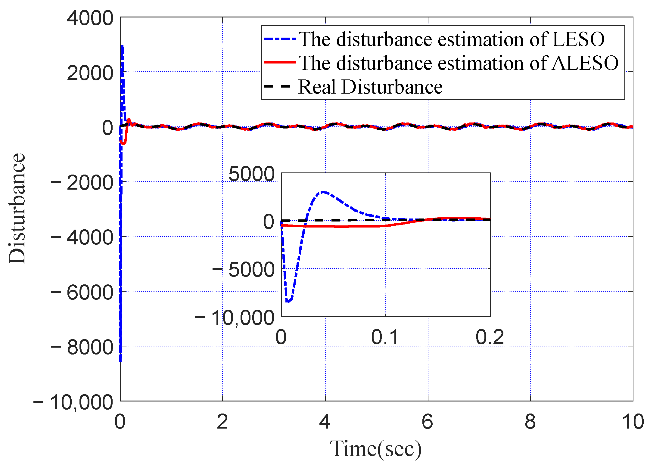
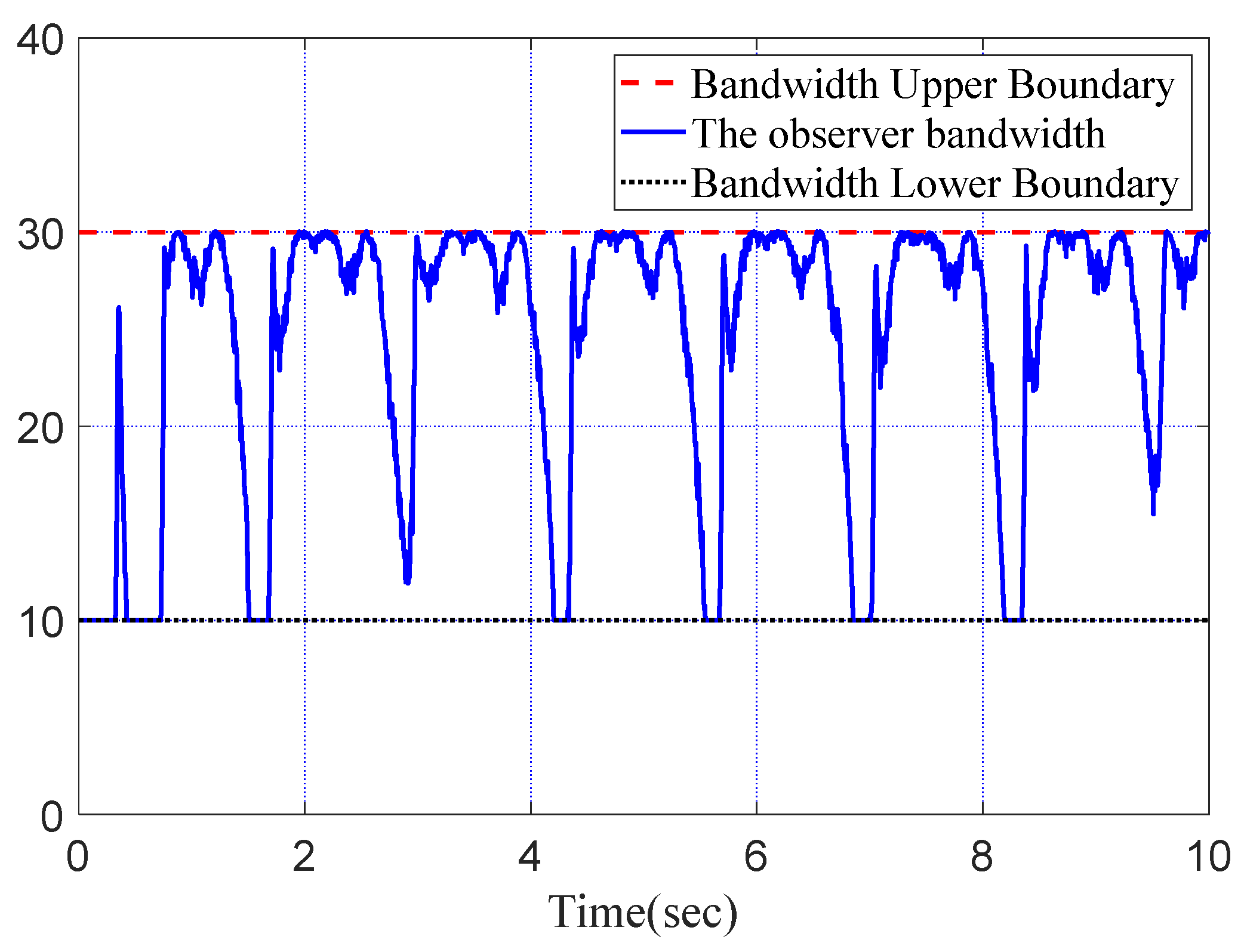
Figure 5,
Figure 6 and
Figure 7 show that the disturbance estimations of LESO and ALESO can track the disturbance within 0.15 s. Due to the continuous adaptive adjustment of the observation bandwidth and the disturbance estimation compensation, the estimation value of ALESO can deal with the peaking phenomenon without introducing excessive noise and can maintain a good estimation performance. Compared with the LESO, the ALESO has a better estimation accuracy. The maximum peak of estimation of ALESO is 621.3. That is only 7.24% of that of the former. In addition, the maximum disturbance estimation error of ALESO is around 20. That is only 33.4% of that of the former. At the beginning of the simulation, due to the large deviation between the initial states
,
of the ISP system and the estimated states
,
of the ALESO, from
Figure 7 it can be seen that the bandwidth
was less than 0.5 s, and the
gradually reached the maximum value
with the decrement of the estimation errors
,
.
4.2. Experiments
Case 1: Vehicle Experiment
To further validate the performance of the proposed method, a vehicle experiment was carried out in the presence of linear motion, angular motion and vibration. The desired attitude angle
was set to
to evaluate the disturbance rejection performance. As a comparison, the results obtained by the adaptive radial basis function neural network and back-stepping sliding mode control method (ANNSMC) of [
25] is also displayed. In the vehicle experiment, the proposed method and ANNSMC were tested on a similar road and at a similar velocity.
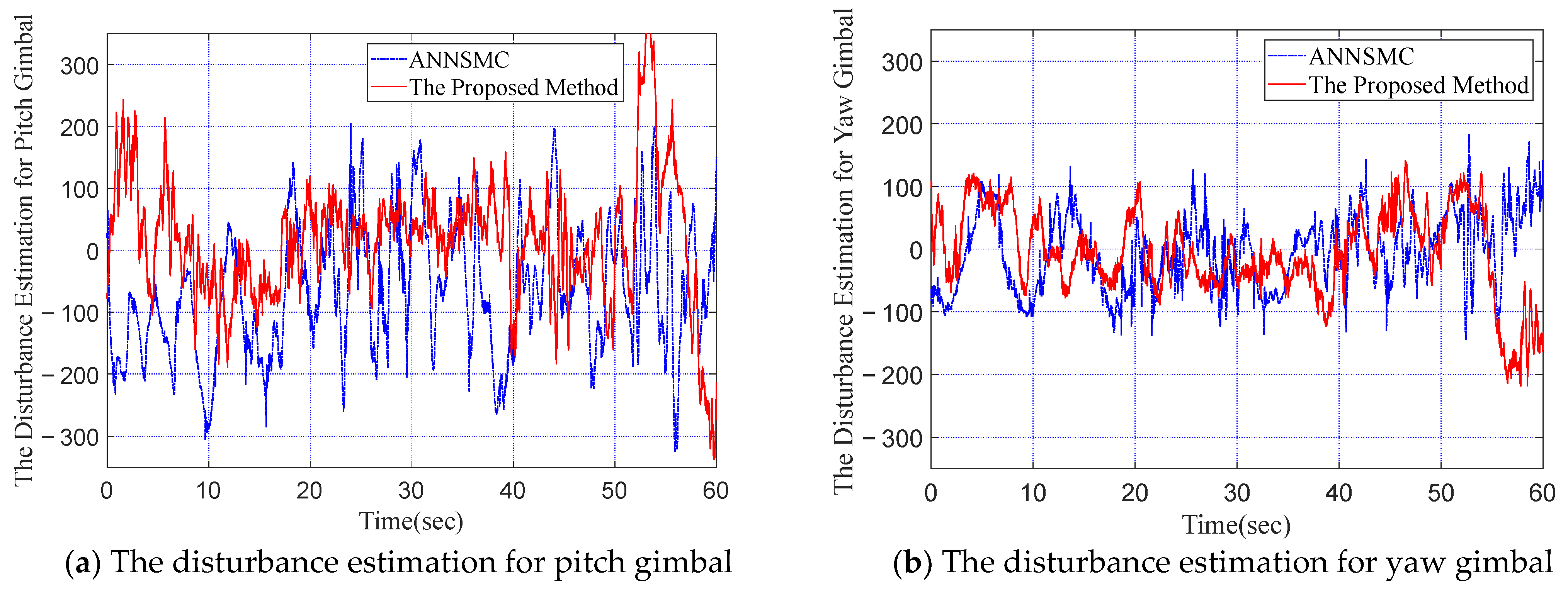
Control performances, control voltages and disturbance estimations are shown in
Figure 8,
Figure 9 and
Figure 10. According to
Figure 8,
Figure 9 and
Figure 10, both the proposed method and the ANNSMC could estimate the disturbance, and the control voltages of them are both around ±2 V, which facilitates the ISP system to run longer.
Table 3 shows RMSE, ITAE and MAXE values of the two controllers. Obviously, compared with the ANNSMC, RMSE value of the proposed method is improved at least 21.4%, ITAE value of the proposed method is improved at least 22.2%, and MAXE value of the proposed method is improved at least 13.8%.
Table 3 shows that the proposed control method has the better control performance in Case 1.
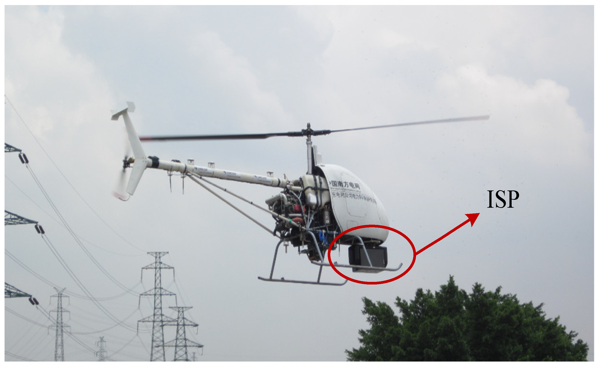
Case 2: Flight Experiment
To verify the effectiveness of the proposed method against complex disturbances, the intelligent inspection system finished a series of inspection tasks for 500 KV high voltage lines. The intelligent inspection system of the UH and ISP is shown in
Figure 11. The ISP system is mounted at the bottom of the UH.
The whole length of the high-voltage wire is 28 km. In addition, there are 12 electronic towers that should be inspected. Between two towers, the UH flew with the speed of 8 m/s. Based on the GPS information of the high voltage tower and UH, the ISP automatically generates adjustment angle information. Then, the ISP was adjusted to track the high-voltage wire to get corresponding images. When the UH came to the nearby region of the tower, the speed of the UH was decreased to 2 m/s. At the same time, the ISP was adjusted to desired orientations for image acquisition. Each side of the high voltage tower was photographed and 3×5 photos were taken as a database for autonomous fault location. Since the long focus camera and short focus camera, infrared camera, ultraviolet camera, 3D laser scanner, and the POS were located in the settled positions of the pitch gimbal, the output of the POS was used as the criteria of the ISP system. To make a clear inspection for the high voltage tower, the common angular motion range of the pitch gimbal was from −70° to 10° because the common height of the 500 KV high voltage tower is 35 m. In addition, the common angular motion range of the pitch gimbal was 0° to 250°, due to consideration of energy consumption. For the ISP system, the pointing accuracy and quick response ability are the two main criteria in the task-finishing process.
The corresponding attitude angles of two gimbals generated by the proposed control method are shown in
Figure 12 and
Figure 13. For the pitch angle, the MAXE is 0.38° and the dynamic response speed arrived at 97.89°/s. Moreover, the MAXE and RMSE of yaw angle are 0.12°and 0.018°, respectively. The ISP can realize a 40° adjustment of yaw angle in 0.48 s, such that the response speed can reach to 83.33°/s. When the outputs of the POS have come to the planned angles, the ISP can realize a high-performance steady control, such that the MAXE is less than 0.4°, and RMSE is less than 0.02°. Since the shutter time is 1/800 s and there is nearly 4 s to executive tasks for the ISP in steady time, the ISP can realize a fast dynamic response and a high precise stabilization control for the high-voltage line inspection tasks.
The intelligent inspection system finished 35 high-voltage line wire-inspection tasks. A total of 378 faults were located in the inspection process. The located faults of the spontaneous explosion of glass insulator string are shown in
Figure 14.


