Article

Adaptive Swarm Fuzzy Logic Controller of Multi-Joint Lower Limb Assistive Robot

by
Mohammad Soleimani Amiri
1,
Rizauddin Ramli
1,* and
Norazam Aliman
2
1
Department of Mechanical and Manufacturing Engineering, Faculty of Engineering and Built Environment, Universiti Kebangsaan Malaysia, Bangi 43600, Selangor, Malaysia
2
Department of Mechanical Engineering, Politeknik Sultan Azlan Shah, Behrang 35950, Perak, Malaysia
*
Author to whom correspondence should be addressed.
Machines 2022, 10(6), 425; https://doi.org/10.3390/machines10060425
Submission received: 24 April 2022 / Revised: 20 May 2022 / Accepted: 23 May 2022 / Published: 27 May 2022
(This article belongs to the Topic Intelligent Systems and Robotics)

Abstract

:
The idea of developing a multi-joint rehabilitation robot is to satisfy the demands for recovery of lower limb functionality in hemiplegic impairments and assist the physiotherapists with their therapy plans. This work aims at to implement the Lyapunov Adaptive and Swarm-Fuzzy Logic Control (LASFC) strategy of 4-degree of freedom (4-DoF) Lower Limb Assistive Robot (LLAR) application, in which the control law is an integration of swarm-fuzzy logic control (SFLC) and Lyapunov adaptive control (LAC) with particle swarm optimization (PSO). The controller is established based on the sliding filtered steady-state error for SFLC. Its parameters are tuned by using PSO for the mathematical model of LLAR. The fuzzy defuzzification membership is set based on the tuned parameters for the real-time control system. LAC strategy is determined using stability analysis of the system to choose the controller’s parameters by observation of the system’s output and reference. The control law implemented in LLAR is the integration of SFLC and LAC to adjust the input voltage of joints. The parameters tuned by PSO are compared with the genetic algorithm (GA) statistically. In addition, the real-time trajectory tracking of the proposed controller for each joint is compared with LAC and SFLC separately. The experiment revealed that the LASFC has superior performance to the other two methods in trajectory tracking. For example, the average error for left hip by LASFC is 53.57% and 68% lower than SFLC and LAC, respectively. By the statistical analysis, it can be ascertained that the LASFC strategy performed efficiently for real-time control of the joint trajectory tracking.

1. Introduction

The occurrence of neurological diseases such as spinal cord injuries and stroke have increased and have become one of the main reasons for mobility impairments and vestibular dysfunction in many countries [1,2,3]. Adequate rehabilitation training is essential to slow down the disabling effects of chronic health conditions [4]. Recent clinical investigations on neurological rehabilitation have revealed the positive influence of repetitive motor activities on obtaining movement functionality. Traditional rehabilitation methods are physically demanding work, in which physiotherapists are required to deliver manual treatment based on their experiences. Practicing conventional manual therapy is often difficult and needs considerable exertion by practitioners to provide care for large patients [5]. Therefore, the application of robot-assisted rehabilitation devices has increased recently due to their potential in providing repetitive rehabilitation training to avoid muscle atrophy for disabled patients and lessen the physical efforts of the physiotherapists [6]. Integration of robotic technology and clinical rehabilitation treatments provides affordable and efficient long-endurance treatments as an alternative to high-intensity repetitive manual rehabilitation therapy. According to previous work, robot-assisted systems have been investigated in the implementation of a rehabilitation program to assist practitioners and mobility impaired individuals [7,8]. For instance, Franceschini et al. [9] investigated long-term effects of robot-assisted therapy for upper limbs compared with traditional physical therapy on stroked subjects for six months.
The control strategies in rehabilitation robots play a crucial role in retrieving satisfactory performance for various rehabilitation treatments [10]. Several training programs, such as repetitive motion tasks, require predetermined multi-joint trajectories. This type of practice demands precise trajectory control strategies. Numerous control techniques have been used in existing literature [11,12,13]. For instance, Tu et al. [14] presented a control strategy using the adaptive sliding mode method for the 4-degree of freedom (4-DoF) lower limb exoskeleton. Their strategy consisted of two outer loops with admittance parameters for estimating wearer active muscle strength and the inner loop of an adaptive sliding mode controller. Guo et al. [15] investigated model parametric identification for the lower exoskeleton to determine the unknown parameters of the mathematical model by using biogeography-based learning particle swarm optimization (PSO). They also used the active admittance controller for angular trajectory tracking. Yang et al. [16] developed a control scheme based on repetitive learning control and neural network (NN) for the lower limb exoskeleton, and they proved the stability of their control strategy with the Lyapunov approach.
Many researchers focused on combining fuzzy logic and control systems [17,18,19]. Sharma et al. [20] presented a control system that was the integration of a fuzzy logic controller (FLC) and dragon fly optimization algorithm for 4-DoF lower limb exoskeleton. In other work, Wu et al. [21] proposed a novel control strategy for a rehabilitation upper limb exoskeleton based on a neural-fuzzy adaptive control scheme. The output of their controller is a combination of the adaptive neural network, fuzzy logic, and force feedback compensation. It was developed based on sliding filtered steady-state trajectory error and fuzzy inference to determine controller parameters in a real-time control system. Sun et al. [22] studied reduced adaptive fuzzy decoupling control for a lower limb exoskeleton. Their fuzzy inference was developed based on the steady-state of the control system. They validated the control strategy in a multi-input-multi-output uncertain nonlinear system model. Premkumar et al. [23] presented a fuzzy proportional derivative controller and fuzzy proportional derivative integral controller, in which the ranges of defuzzification membership function are determined by a bat optimization algorithm.
From literature [17,18,19,20,21,22,23], there are various types of controller strategies to increase the performance of fuzzy logic on nonlinear systems. Developing a simpler controller strategy with more efficient tracking performance has attracted much attention from researchers. The aim of using fuzzy logic as a control strategy is to minimize the complexity of the control system and reduce processing time and computational burden. This paper presents a new PSO-based initialization for fuzzy logic and adaptive controller in a lower limb assistive robot (LLAR) for passive mode rehabilitation exercise, which is a new approach compared to the previous fuzzy logic and adaptive control strategy.
The novelty of this paper is to implement the Lyapunov Adaptive and swarm-fuzzy logic control (LASFC) strategy on the 4-degree of freedom (4-DoF) LLAR, in which the control law is an integration of swarm-fuzzy logic control (SFLC) and Lyapunov adaptive control (LAC) that are improved by particle swarm optimization (PSO). In summary, the contributions of the paper are:
  • A novel LASFC, which integrates SFLC and LAC strategies, is presented for each joint of the LLAR to achieve the predetermined angular trajectories.
  • A SFLC is developed to tune the parameters of the controller based on sliding filtered steady-state error. Its defuzzification subsets are determined by PSO.
  • A LAC strategy is initialized by PSO to adjust the controller parameters in real-time.
  • The novel LASFC is implemented in the actual 4-DoF LLAR.
The rest of this paper is organized as follows: In Section 2, the structure of the LLAR, the dynamic model, and actuator formulation are given. Section 3 addresses the development of LASFC and the integration of PSO with SFLC and LAC. Section 4 represents the performance and result of the proposed LASFC strategy in real-time control of LLAR. The conclusion is in Section 5.

2. Overview of the LLAR Structure

The mechanical structure, the electrical components, and the mathematical model of LLAR are described herein.

2.1. Mechanical Design and Structure

The LLAR is worn by a human subject in parallel to their lower limb. It has a 4-DoF linkage that consists of two active joints, such as the hip and knee, in each leg. The hip and knee are flexion/extension rotation joints. The structure of the LLAR is shown in Figure 1.
Each joint is operated by a 12 V brushed DC motor and a worm gearbox. The generated torque is transmitted to the worm gearbox with gear ratio of 32. A quadrature encoder is located at the motor shaft to record the angle of each joint with a resolution of 200 pulses per rotation. An Arduino Mega 2560 is used to control and capture the data from the encoder and regulate the input voltage and direction of actuators based on the determined data from the control system. Figure 2 illustrates the structure of hardware of the LLAR.
As can be seen in Figure 2, four DC motor drivers are used to convert the direction and pulse-width modulation (PWM) received from the Arduino to the actuators of each joint. An embedded PC using Raspberry Pi4 8 GB is employed to communicate with the Arduino and the base station. The connection between the Raspberry Pi and the base station is a master PC employed to monitor and command the LLAR through a WiFi hotspot. Robot Operating System (ROS) is used as the master and client for this communication. The control system is programmed in Python and run in the base station, which is a PC with an Intel Core i3 CPU 16 GB RAM.

2.2. Mathematical Analysis of Dynamic Model

The dynamic model of a multi-joint serial-link robot can be determined by a Lagrangian equation. The dynamic equation is expressed as follows:
M ( θ ) θ ¨ + V ( θ , θ ˙ ) + G ( θ ) = τ + F ( t ) + D ,
where M ( θ ) 4 × 4 is the inertia matrix; V ( θ , θ ˙ ) 4 is centripetal and Coriolis vector; G ( θ ) 4 introduces the gravitational force; τ 4 represents the torques generated by actuators; F ( t ) 4 is vector of interactions between human subject and exoskeleton; and D 4 denotes uncertainties, including external disturbances, modelling errors, and frictional forces.
In general, the following properties hold for the exoskeleton dynamic system: [16]
Property 1. 
The inertia matrix M 4 × 4 is positive-definite and symmetric inertia, which is further bounded,
α 1 x 2 < x T M ( θ ) x < α 2 x 2 , x , θ 4
where α 1 and α 2 are the positive constants and . is the standard Eulidean norm.
Property 2. 
The centripetal and Coriolis vector V ( θ , θ ˙ ) 4 and the time derivative of the inertia matrix M ( θ ) 4 × 4 satisfy the following equation:
x T [ M ˙ ( θ ) 2 V ( θ , θ ˙ ) ] x = 0 , θ , θ ˙ 4 .
Property 3. 
The uncertain term D 4 is limited by positive constant δ as follows:
D < δ .

2.3. Actuator Model

The joints of the exoskeleton are actuated by DC motors to provide the required torque. The input voltage is determined as follows:
u = L ( d i d t ) + R i ,
where L and i represent the electric inductance and current, respectively; R and u are resistance and the input voltage of the DC motor, respectively. The generated torque is proportional to the current as follows:
τ m = K m i ,
where K m is the torque sensitivity. In addition, the generated torque by the DC motor applied to the joints is the summation of link torque τ l and rotary torque τ r , given as follows:
τ m = τ r + τ l ,
where τ r is the torque of the rotary shaft, which is given as follows:
τ r = J θ ¨ + C f θ ˙ ,
where J and C f represent the inertia of the rotary shaft and friction coefficient. The mathematical model of the LLAR in continuous time is written as follows:
G i ( s ) = θ ( s ) u ( s ) = b i a 1 i s 3 + a 2 i s 2 + a 3 i s + a 4 i
where G i ( s ) denotes the mathematical model of the hip and knee; b i and a j i , j = 1 , 2 , 3 , 4 are the parameters. The mathematical model was determined previously in [24] by system identification determined by genetic algorithm (GA) to estimate the parameters of the mathematical model. As the LLAR has symmetric parallel legs, we consider one leg for developing the control strategy. Table 1 expresses the mathematical model parameters for hip and knee joints.

3. Development of Lyapunov Adaptive Swarm-Fuzzy Logic Control Strategies

3.1. Overview of Control Strategy

To design the LASFC strategy, the control law is composed of two terms: LAC and SFLC. The overall block diagram of the LASFC control strategy is shown in Figure 3.
Therefore, the output of LASFC u is expressed as follows:
u = u f + u a ,
where u f and u a are the output of LAC and SFLC, which are developed by the Lyapunov approach and if-and-then linguistic rules. The control task for LLAR is to bound the controller output u that the output trajectory track x the desired trajectory r as minimally as possible despite uncertainties and disturbances.
In the LASFC strategy, the parameters of the fuzzy control law are pre-tuned by PSO. The tuned parameters determine the defuzzification subsets ranges. The control law is defined based on the observation of the input and output of the system. The tuned parameters are employed as the initial value for control law determined by the Lyapunov approach. Algorithm 1 shows the implementation method of LASFC.
Algorithm 1 Pseudo code of LASFC.
1:
Start;
2:
Establish PSO for tuning SFLC control law;
3:
Determine the range of deffuzification subsets;
4:
Set fuzzy logic inference for SFLC;
5:
Establish PSO for tuning LAC control law;
6:
Determine LAC by using Lyapunov stability approach;
7:
Combine SFLC and LAC as the LASFC;
8:
Implement LASFC for LLAR joints;
9:
End.

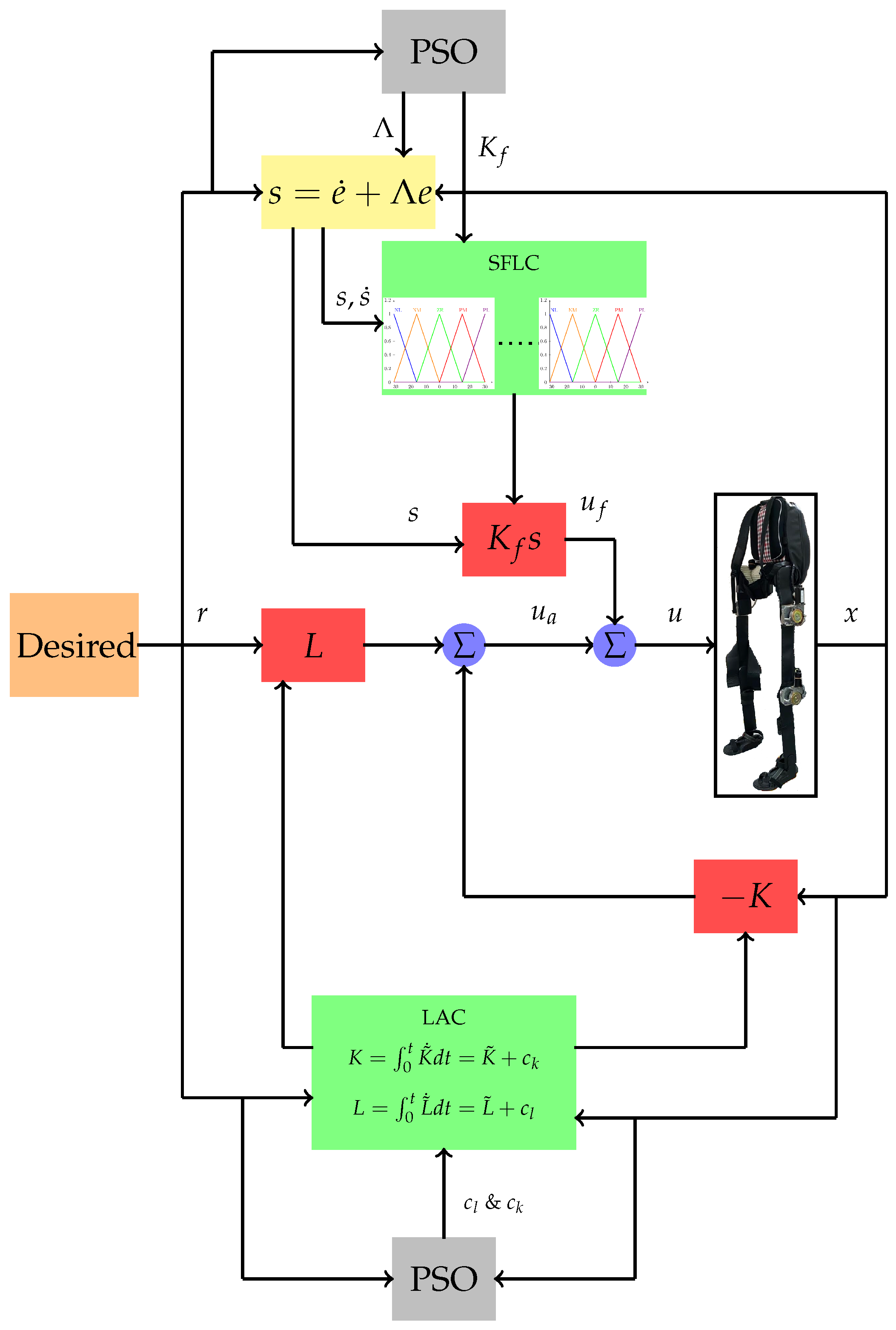
3.2. Swarm-Fuzzy Logic Control Strategy

SFLC adjusts the controller parameters according to the actual situation detected and signal processed by the control system. In this control strategy, the conditions are implemented into fuzzy logic rules that process the data captured by the sensor. Fuzzy inference is then applied, and the actual control parameters can be obtained. The fuzzy logic rules for the inference are captured by PSO, which is used to tune the controller parameters and distinguish fuzzy membership subsets. The PSO is an iterative optimization method based on the population that took its inspiration from observation of biological societies such as a flock of birds, swarms of bees, and schools of fish [25]. Moreover, PSO has a simple concept and is easy to implement in different optimization problems. In addition, it is possible to control the robustness of its parameters. PSO has few parameters to adjust, and it has a high probability of and efficiency in finding the global optimum. The PSO has a chance of finding the global optimum by providing a wide exploration area in the initial iterations to find the neighbor of the global optima and narrowing the searching space to find the best result [26,27]. It causes fast convergence and prevents it from being trapped to the local optimum, which makes it superior to various metaheuristic optimization methods, such as the grey wolf optimizer, whale optimization algorithm, and Jaya algorithm [28].
Fuzzy logic is divided into three main parts: fuzzification, fuzzy inference machine, and defuzzification. Fuzzification is the input of the fuzzy control system, which produces the fuzzy quantity from the transformation of membership sets for fuzzy inference. Let us define A as a fuzzy set, with the membership function characterized as follows:
A = { y , μ ( y ) | y Y , μ ( y ) [ 0 , 1 ] } ,
where Y is the universal base set. α is the subset of set A, represented as follows:
A α = { y , | μ ( y ) α , α [ 0 , 1 ] } .
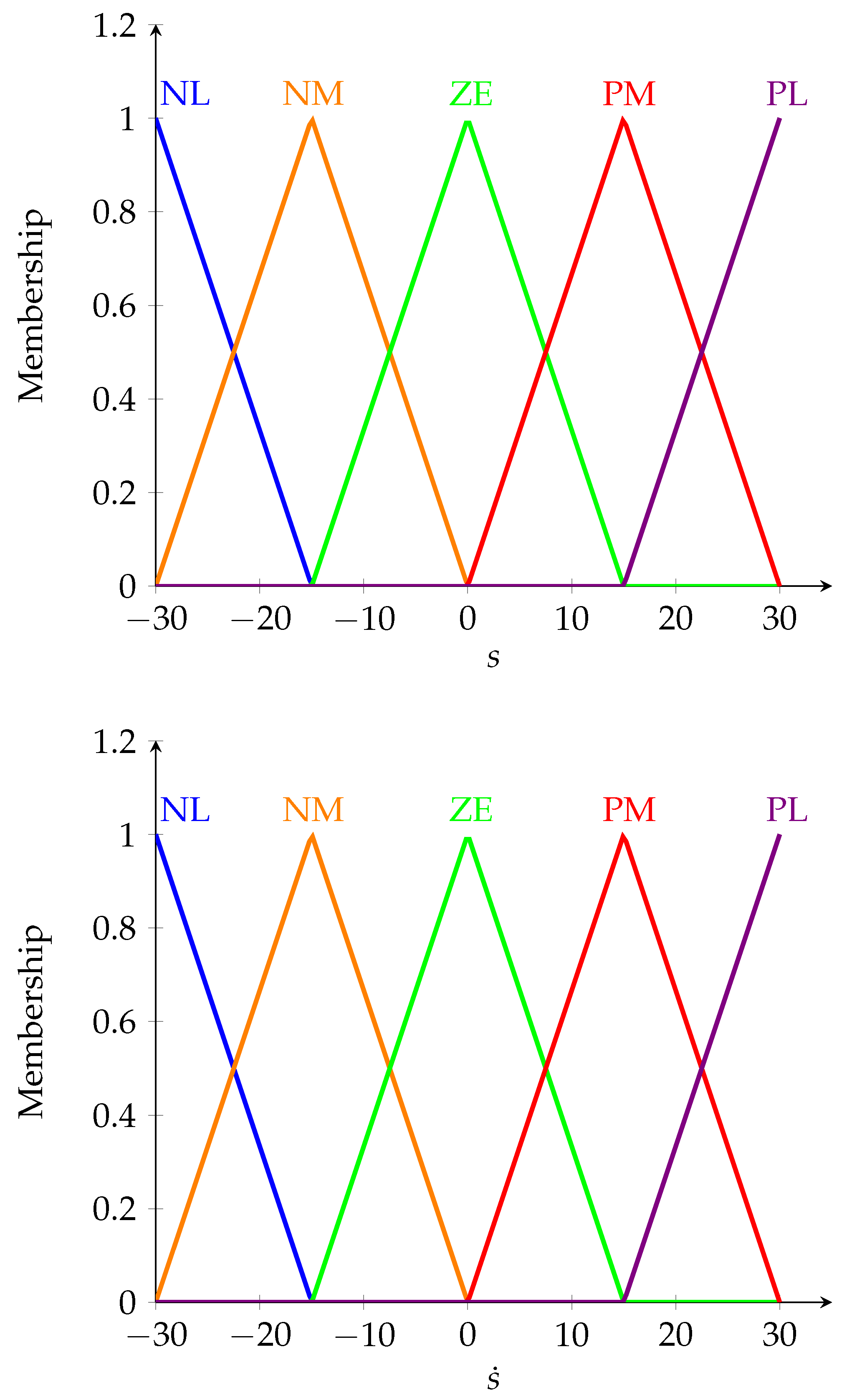
There are several common types of membership functions, including triangular, trapezoidal, and Gaussian, and their graphs have different shapes.
The fuzzy inference machine synthesizes the obtained data from fuzzification and the defined linguistic if-and-then rules. The fuzzy inference is the kernel of fuzzy logic that processes the antecedent as the input by linguistic rules and concludes the consequent output.
Defuzzification is the process of converting the linguistic results of fuzzy inference to the actual quantitative and reasonable crisp values as the output of the fuzzy logic control. This can be achieved by various methods, such as the center of gravity, weighted average, the center of the largest area, and centroid methods. The control law for SLFC controller is given as follows:
u f = K f s ,
where K f is the controller parameter and s represents the sliding filtered steady-state error as follows:
s = e ˙ + Λ e ,
where Λ 4 is the symmetric positive constant gain matrix; e and e ˙ are steady-state error and its derivative as follows:
e = r x , e ˙ = d e d t ,
where r and x are the desired and actual angular trajectories. The tuning of controller parameters K f and Λ are defined as the optimization problem and solved by PSO. The objective function of the optimization problem is integral time absolute error (ITAE) for the closed-loop control system, in which the controller is shown in Equation (13) and the plant is the hip and knee mathematical models. The objective function is expressed as follows:
f ( e , t ) = 0 t t | e | d t ,
where t is elapsed time. Each particle of the PSO consists of design variables of controller parameters K f and Λ . The initial particles are filled by random values between zero and one.
x 1 , j [ 0 , 1 ] j = 1 , 2 , , μ
where j and μ are the number and maximum quantity of particles. The objective function is determined for each particle for evaluation. The minimum one is selected as the best particle, denoted as p. The particles of the next generations are created by the summation of the current particle and the velocity of each particle, expressed as follows:
x i , j = x i 1 , j + υ i , j
where i is the number of iterations; υ i , j carries the velocity and direction of each particle toward the particles of the next iteration [29]. The value of υ i , j is given as follows:
υ i , j = ω υ i 1 , j + c 1 ζ ( p i 1 x i , j ) + c 2 ζ ( g x i , j )
where ω is positive constant of inertial weight, and c 1 and c 2 are self and social recognition positive constants; g represents the best global particle determined after evaluation of particles in each iteration in comparison with the best particle p; ζ is a random value between 0 and 1. The particles captured as global best g of the last iteration are the optimal output of the algorithm.
ζ [ 0 , 1 ]
The parameters of the PSO is expressed in Table 2.
To tune the controller parameters K f and Λ , the noted optimum problem is solved by PSO and compared by GA and beetle antennae search (BAS). The elapsed time is 10 s and the time step is 0.1 s. The population and generation numbers for GA and BAS are 20 and 200, respectively. Table 3 compares numerical analysis of PSO and GA in the unit step response closed-loop control system for an LLAR hip joint.
The average of ITAE driven by PSO for ten different runs are 34.8% and 63.13% less than GA for hip and knee, respectively. Moreover, this value for PSO is 18% and 56% lower than BAS for hip and knee, respectively. Therefore, the controller parameters tuned by PSO are selected. The p-value comes from the ANOVA test for the ITAE of ten different running by PSO and GA. The p-value is lower than 0.005, which shows the ITEA for ten different runs is not repetitive.
Therefore, in the real-time control of the LLAR, the controller parameters K f and Λ are chosen as follows:
  • Λ is the constant value tuned by PSO. Its average values in Table 3 are selected for hip and knee, which are 0.88 and 0.76, respectively.
  • K f 
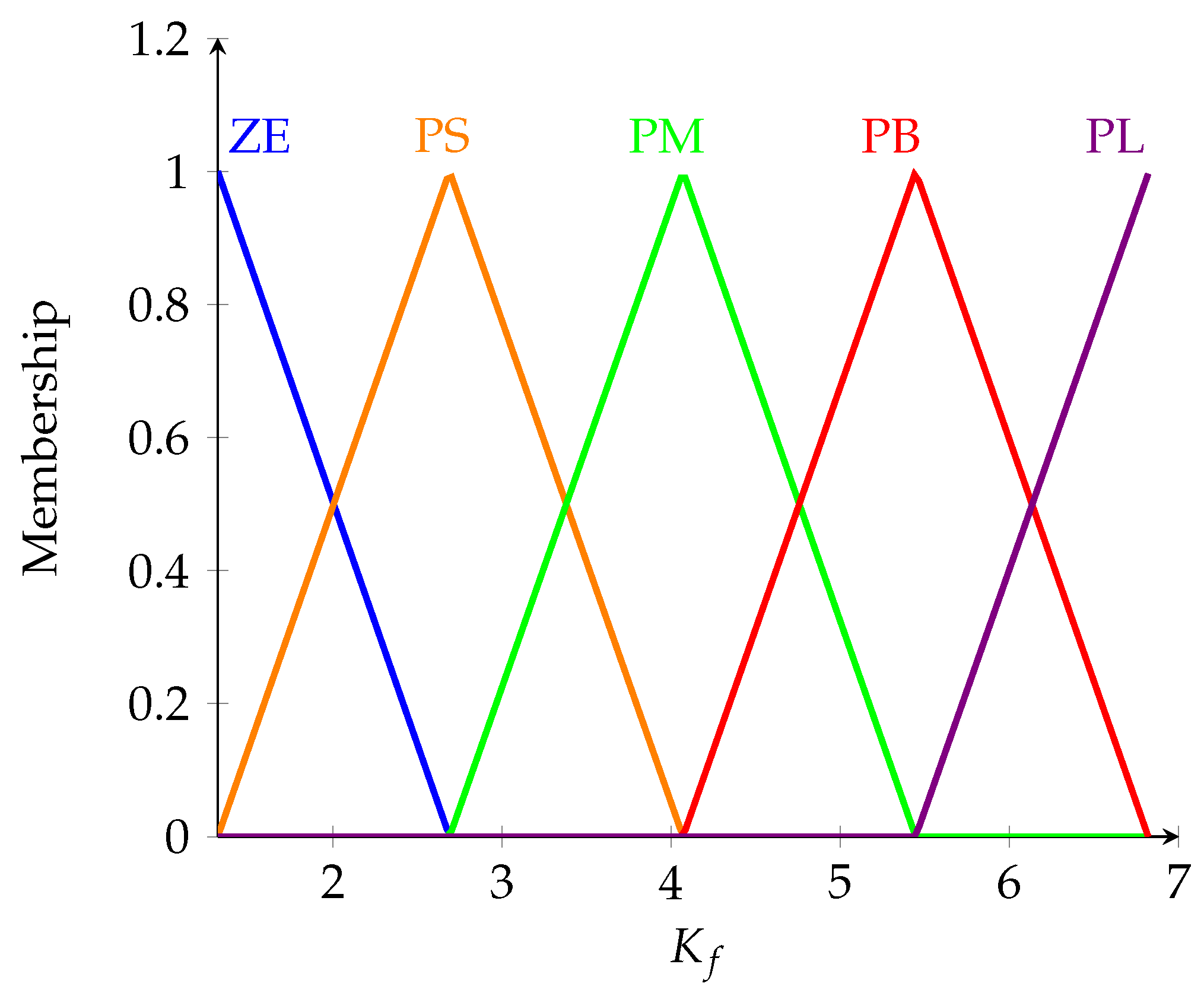
is the output of the fuzzy inference. It is determined by the linguistic rules of the fuzzy controller based on its maximum and minimum obtained by PSO in Table 3, which are 6.82 and 1.32 for hip and 6.95 and 2.64 for knee.
The parameter K f is the output of the fuzzy inference by the linguistic rules and fuzzy sets. Five subsets are defined for K f defuzzification membership function such as ZE, PS, PM, PB, and PL, in which their ranges are determined based on minimum and maximum of K f driven by PSO, given as follows:
T [ K f m i n , K f m i n + q K ´ f ] , q = 0 , , n
where T represents the defuzzification subsets; n denotes the number of defuzzification subsets; and K ´ f is the defuzzification subsets range step, expressed as follows:
K ´ f = K f m a x K f m i n n 1 .
The linguistic fuzzy logic rules are defined based on sliding filtered error s and its derivative, as expressed in Table 4. Defuzzification subsets are as: Zero (ZE), Positive Small (PS), Positive Medium (PM), Positive Big (PB), and Positive Large (PL).
The fuzzy logic rules are defined as follows:
i f s i = L i & s ˙ = H i t h e n K f = T i
where L i and H i are the input fuzzy subsets labels; and T i represents output fuzzy subsets. Particularly, there are two examples of the fuzzy logic rules, written as follows:
i f s i = N L & s ˙ = Z E t h e n K f = Z E
i f s i = P M & s ˙ = N M t h e n K f = P M .
The center of gravity technique and Zadeh fuzzy synthesis method are employed for fuzzy defuzzification [30]. Pseudo code of SLFC is illustrated in Algorithm 2.
Algorithm 2 Pseudo code of SLFC
1:
Input variables: i = 400 , c 1 = 2 , c 2 = 2 , ω = 1.2 and μ = 20
2:
_________________________________________________________
3:
Output variables: Λ , K f , and  f ( e , t ) ;
4:
_________________________________________________________
5:
Start;
6:
Initialize particles by random values;
7:
Evaluate initial population;
8:
Select the initial p;
9:
while (Number of iteration less than μ ) do;
10:
    Create new iteration;
11:
    Update velocity and position;
12:
    Select the p;
13:
    if p less than the previous g then;
14:
        Store it as g;
15:
    end if
16:
end while
17:
Select the particle of g as the result;
18:
Determine Λ for control law;
19:
Set fuzzification and defuzzification linguistic rules;
20:
Set fuzzification membership function for s and s ˙ ;
21:
Determine K ´ f based on the results of PSO;
22:
Implement the defuzzification membership function for K f ;
23:
End.
Figure 4 and Figure 5 illustrate membership functions for input and output for the SLFC for the hip.

3.3. Lyapunov Adaptive Control Strategy

LAC is defined to guarantee the stability of the non-linear dynamic system by the Lyapunov approach. It is mainly used in the control system to improve robustness in the presence of external forces. To clarify, consider the case that the LLAR is worn by the human object, hence the desired torque should be generated to minimize the steady-state-error e thus the auxiliary variable x converges to zero [31,32].
Theorem 1. 
Consider a non-linear dynamic system,
x ˙ = f ( x ) , x n , f ( 0 ) = 0
where f is a Lipschitz function. Consider a function V : n [ 0 , ) , which is a positive definite function and V x is a Lipschitz gradient. The Lyapunov function for a system is considered as follows [33]:
V ˙ : = V x · f ( x ) < 0 , x 0 .
Such a system is stable if the Lyapunov function V exists and its derivative is negative definite.
Proof. 
By considering Equation (9), the state-space variables are assumed as follows:
X 1 = θ ,
X 2 = θ ˙ = X ˙ 1 ,
X 3 = θ ¨ = X ˙ 2 .
Therefore, the time-invariant vector differential of LLAR mathematical model is given as follows:
X ˙ = A X + B u a ,
the control law is selected to observe the reference and output of the control system given as follows:
u a = K x + L r .
Here, the candidate Lyapunov function is chosen as follows:
V ( x ) = X T ˙ P X + K ˜ T Γ 1 K + L ˜ T Γ 1 L
where P is a positive definite matrix used to simplify algebra without any loss of generality; X T ˙ is the transpose of Equation (31); and Γ is the adaptation gain matrix, which is positive definite. Differentiating Equation (33) over time, it can be obtained,
V ˙ ( x ) = X T ˙ P X + X T P X ˙ + K ˜ ˙ T Γ 1 K ˜ + K ˜ T Γ 1 K ˜ ˙                                             + L ˜ ˙ T Γ 1 L ˜ + L ˜ T Γ 1 L ˜ ˙
where K ˜ = K K ^ and L ˜ = L L ^ , in which K ^ and L ^ are the estimation of controller parameters. Therefore,
K ˜ ˙ T Γ 1 K ˜ = K ˜ T Γ 1 K ˜ ˙
L ˜ ˙ T Γ 1 L ˜ = L ˜ T Γ 1 L ˜ ˙
from Equation (31),
X ˙ T = X T A T + B T u a .
Substituting Equation (31) into Equation (34), we can get,
V ˙ ( x ) = ( X T A T + B T u a ) P X + X T P ( A X + B u a )                                         + 2 K ˜ ˙ T Γ 1 K ˜ + 2 L ˜ ˙ T Γ 1 L ˜
Substituting Equation (32) into Equation (38) and simplifying, it can be given
V ˙ ( x ) = X T ( A T P + P A ) X + K ˜ ( B X P X X T P B X + 2 K ˜ ˙ T Γ 1 )                                                       + L ˜ ( B T r P X + X T B r + 2 L ˜ ˙ T Γ 1 ) .
It is assumed for a given positive-definite matrix Q, there is a positive-definite solution P such that P A + A T P = Q . Thus, if the expressions B X P X X T P B X + 2 K ˜ ˙ T Γ 1 and B T r P X + X T B r + 2 L ˜ ˙ T Γ 1 converge to zero, the differential of Lyapunov function will be V ˙ = X T Q X , which is the negative, and Theorem 1 is satisfied.
Therefore, the parameters of controller are given as follows:
K ˜ ˙ = Γ ( B X P X + X T P B X ) 2
L ˜ ˙ = Γ ( B r P X + X T P B r ) 2 .
By applying the time domain integral of Equations (41) and (40), the parameters of the adaptive control system are represented as follows:
K = 0 t K ˜ ˙ d t = K ˜ + c k
L = 0 t L ˜ ˙ d t = L ˜ + c l
where c k and c l are the unknown parameters, which are determined by optimal tuning by PSO. The objective function of the PSO is ITAE, which is determined in the closed-loop control system by the control law given in Equation (32). The design variables are the two control parameters. The parameters of PSO are shown in Table 2. Table 5 compares the optimal results for c k and c l determined by PSO, GA, and BAS. The population and generation numbers for GA and BAS are 20 and 200, respectively.
The average of ITAE determined by PSO for ten different runs is 32.14% and 69.4% less than GA for hip and knee, respectively. This value for PSO is 50% and 71.1% lower than BAS. Hence the optimal results that have the lowest ITAE established by PSO for hip and knee are selected as c k and c l .

4. Results and Discussion

The performance of the proposed LASFC is validated for LLAR joints. In addition, its efficiency is compared with LAC and SFLC separately. The angular trajectory tracking test is suggested to evaluate the performances of the proposed LAC, SFLC, and LASFC. The desired trajectories are developed for the rehabilitation gait training exercise inspired by the stand and swing phases of healthy human walking [34]. The desired trajectories equations for left hip, left knee, right hip, and right knee, respectively, are given as follows:
y l h ( t ) = m a x ( 0 , 20 s i n ( f t ) ) ,
y l k ( t ) = m i n ( 0 , 30 s i n ( f t + π ) ) ,
y r h ( t ) = m a x ( 0 , 20 s i n ( f t + π ) ) ,
y r k ( t ) = m i n ( 0 , 30 s i n ( f t ) ) ,
where t and f are the elapsed time and frequency. Figure 6 compares the angular trajectories LAC, SFLC, and LASFC for four joints of LLAR.
As can be seen in Figure 6, LASFC converged to the desired trajectory more efficiently than LAC and SFLC, due to the parameters adjustment and initialization by PSO. In all joints, the error of LASFC has the lowest peak. The parameter’s range for defuzzification of SFLC is adjusted by PSO tuning technique, despite the fact that the LAC parameters are initialized by the PSO and it should adjust the parameters based on the observation of output and input of the control system. Therefore, SFLC performed better than LAC. Figure 7 represents the changes of fuzzy parameter for LASFC strategy for the left hip and knee.
In Figure 7, K f changes periodically based on the swing and stand phases of left hip and knee trajectories. It raises with fluctuation while the trajectory is in the swing phase to converge the trajectory error. In addition, it levels off while the angular trajectory is stable in the standing phase for the hip and knee. Figure 8 shows K f changes over s and s ˙ for four joints determined by LASFC strategy.
In Figure 8, it can be observed how the fuzzy logic rules are followed by LASFC. For instance, s and s ˙ are in the NL and NM fuzzy subset ranges, whereas K f is in its highest range, which are PL and PB fuzzy subsets. In addition, while s and s ˙ increase, the K f moves to its lower subsets. Figure 9 illustrates the changes of L and K parameters of the adaptive controller strategy of LASFC for the left hip and knee.
In Figure 9, the parameters of L and K reached their peak when the angular trajectories are in the swing phase of gait training. They remain constant in the initialized value tuned by PSO for LAC. Table 6 represents a statistical analysis of angular trajectory error determined by LAC, SFLC, and LASFC.
In Table 6, E m a x , E a v e , and RMS denote maximum, average, and root mean square steady-state error, respectively. The E m a x , E a v e , and RMS for LASFC are significantly lower than for LAC and SFLC. For example, the E a v e for the left hip by LASFC is lower than than SFLC and LAC by 0.013 (rad) and 0.028 (rad), respectively. In addition, E m a x for the right knee determined by LASFC is 0.012 (rad) and 0.066 (rad) lower than SFLC and LAC. Generally, E m a x , E a v e , and RMS calculated by LASFC did not exceed 0.05 (rad), which is the acceptable value [35]. Table 7 compares the performance of LASFC with three other controllers for exoskeletons.
For the current study, IAE is lower than the NN-based controller demonstrated in [37] and FLC presented in [30] by 85% and 62% for the hip joint, respectively. It should be considered that the exoskeleton model demonstrated in [30] was developed in Matlab/Simulink as the benchmark and was not validated in the experimental prototype. In addition, the RMSE in this work is 28% lower than PSO-PID represented in [36] for the knee. The actuator used in [36] is BLCD Maxon, which has higher quality and power than the motor used in the present work.

5. Conclusions

This paper presented a novel LASFC strategy based on the integration of the LAC and SFLC for LLAR. In FSLC, the defuzzification membership function for parameters of the controller was determined based on the PSO. Similarly, the parameters of the LAC controller were initialized by PSO. The results comparison of LAC, SFLC, and LASFC showed satisfactory performance for the three control strategies, despite the LASFC performing more accurately with lower steady-state error. For instance, the E a v e for the left hip by LASFC is 53.57% and 68% less than SFLC and LAC, respectively. In addition, E a v e for the right knee determined by LASFC is 45% and 70% lower than SFLC and LAC.
The proposed LASFC strategy can be implemented in multi-joint exoskeleton robots for assisting physiotherapists in rehabilitation training. However, this method is validated in the fixed frame of LLAR for specific average height subjects. In addition, human-in-loop effects for various rehabilitation exercises have not been considered in this paper. By considering these limitations in future work, the effect of the wearer’s forces will be added to the controller strategies and it will be tested in a variety of rehabilitation exercises.

Author Contributions

Conceptualization, M.S.A. and R.R.; methodology, M.S.A., R.R., and N.A.; software, M.S.A.; validation, M.S.A., R.R., and N.A.; formal analysis, M.S.A., R.R., and N.A.; investigation, M.S.A. and R.R.; resources, M.S.A.; data curation, M.S.A. and R.R.; writing—original draft preparation, M.S.A.; writing—review and editing, M.S.A. and R.R.; visualization, M.S.A.; supervision, R.R.; project administration, R.R.; funding acquisition, R.R. All authors have read and agreed to the published version of the manuscript.

Funding

The authors would like to thank Universiti Kebangsaan Malaysia (UKM) for financial support received under research grants KK-2020-014 and DPK-2020-015.

Conflicts of Interest

The authors declare no conflict of interest.

References

  1. Kimura, T.; Horikoshi, Y.; Kuriyagawa, C.; Niiyama, Y. Rho/rock pathway and noncoding rnas: Implications in ischemic stroke and spinal cord injury. Int. J. Mol. Sci. 2021, 22, 11573. [Google Scholar] [CrossRef] [PubMed]
  2. Kang, Y.; Ding, H.; Zhou, H.; Wei, Z.; Liu, L.; Pan, D.; Feng, S. Epidemiology of worldwide spinal cord injury: A literature review. J. Neurorestoratology 2017, 6, 1–9. [Google Scholar] [CrossRef] [Green Version]
  3. Lin, P.H.; Dong, Q.; Chew, S.Y. Injectable hydrogels in stroke and spinal cord injury treatment: A review on hydrogel materials, cell-matrix interactions and glial involvement. Mater. Adv. 2021, 2, 2561–2583. [Google Scholar] [CrossRef]
  4. Shukun, H.; Gang, W.; Zhouying, W.B.D.; Yi, Z. Rehabilitative training paired with peripheral stimulation promotes motor recovery after ischemic cerebral stroke. Exp. Neurol. 2022, 349, 113960. [Google Scholar] [CrossRef]
  5. Hazle, C.R.; Lee, M. Strategies to overcome size and mechanical disadvantages in manual therapy. J. Man. Manip. Ther. 2016, 24, 120–127. [Google Scholar] [CrossRef] [Green Version]
  6. Zhou, J.; Yang, S.; Xue, Q. Lower limb rehabilitation exoskeleton robot: A review. Adv. Mech. Eng. 2021, 13, 16878140211011862. [Google Scholar] [CrossRef]
  7. Lambercy, O.; Ranzani, R.; Gassert, R. Chapter 15—Robot-assisted rehabilitation of hand function. In Rehabilitation Robotics; Colombo, R., Sanguineti, V., Eds.; Academic Press: Cambridge, MA, USA, 2018; pp. 205–225. [Google Scholar] [CrossRef]
  8. Li, Z.; Zhao, K.; Zhang, L.; Wu, X.; Zhang, T.; Li, Q.; Li, X.; Su, C.Y. Human-in-the-Loop Control of a Wearable Lower Limb Exoskeleton for Stable Dynamic Walking. IEEE/ASME Trans. Mechatron. 2021, 26, 2700–2711. [Google Scholar] [CrossRef]
  9. Franceschini, M.; Mazzoleni, S.; Goffredo, M.; Pournajaf, S.; Galafate, D.; Criscuolo, S.; Agosti, M.; Posteraro, F. Upper limb robot-assisted rehabilitation versus physical therapy on subacute stroke patients: A follow-up study. J. Bodyw. Mov. Ther. 2020, 24, 194–198. [Google Scholar] [CrossRef]
  10. Shi, D.; Zhang, W.; Zhang, W.; Ding, X. A Review on Lower Limb Rehabilitation Exoskeleton Robots. Chin. J. Mech. Eng. English Ed. 2019, 32, 1–11. [Google Scholar] [CrossRef] [Green Version]
  11. Fuentes-Alvarez, R.; Hernandez, J.H.; Matehuala-Moran, I.; Alfaro-Ponce, M.; Lopez-Gutierrez, R.; Salazar, S.; Lozano, R. Assistive robotic exoskeleton using recurrent neural networks for decision taking for the robust trajectory tracking. Expert Syst. Appl. 2022, 193, 116482. [Google Scholar] [CrossRef]
  12. Taherifar, A.; Vossoughi, G.; Ghafari, A.S. Assistive-compliant control of wearable robots for partially disabled individuals. Control Eng. Pract. 2018, 74, 177–790. [Google Scholar] [CrossRef]
  13. Jabbari Asl, H.; Narikiyo, T.; Kawanishi, M. Neural network-based bounded control of robotic exoskeletons without velocity measurements. Control Eng. Pract. 2018, 80, 94–104. [Google Scholar] [CrossRef]
  14. Tu, Y.; Zhu, A.; Song, J.; Shen, H.; Shen, Z.; Zhang, X.; Cao, G. An adaptive sliding mode variable admittance control method for lower limb rehabilitation exoskeleton robot. Appl. Sci. 2020, 10, 2536. [Google Scholar] [CrossRef] [Green Version]
  15. Guo, Q.; Chen, Z.; Yan, Y.; Xiong, W.; Jiang, D.; Shi, Y. Model Identification and Human-robot Coupling Control of Lower Limb Exoskeleton with Biogeography-based Learning Particle Swarm Optimization. Int. J. Control. Autom. Syst. 2022, 20, 589–600. [Google Scholar] [CrossRef]
  16. Yang, Y.; Huang, D.; Dong, X. Enhanced neural network control of lower limb rehabilitation exoskeleton by add-on repetitive learning. Neurocomputing 2019, 323, 256–264. [Google Scholar] [CrossRef]
  17. Liu, F.; Wang, H.; Shi, Q.; Wang, H.; Zhang, M.; Zhao, H. Comparison of an ANFIS and Fuzzy PID Control Model for Performance in a Two-Axis Inertial Stabilized Platform. IEEE Access 2017, 5, 12951–12962. [Google Scholar] [CrossRef]
  18. Qu, Z.; Wei, W.; Wang, W.; Zha, S.; Li, T.; Gu, J.; Yue, C. Research on Fuzzy Adaptive Impedance Control of Lower Extremity Exoskeleton. In Proceedings of the 2019 IEEE International Conference on Mechatronics and Automation, Tianjin, China, 4–7 August 2019; pp. 939–944. [Google Scholar]
  19. Ali, J.A.; Hannan, M.A.; Mohamed, A.; Abdolrasol, M.G.M. Fuzzy logic speed controller optimization approach for induction motor drive using backtracking search algorithm. Measurement 2016, 78, 49–62. [Google Scholar] [CrossRef]
  20. Sharma, R.; Gaur, P.; Bhatt, S.; Joshi, D. Optimal fuzzy logic-based control strategy for lower limb rehabilitation exoskeleton. Appl. Soft Comput. 2021, 105, 107226. [Google Scholar] [CrossRef]
  21. Wu, Q.; Xingsong, W.; Bai, C.; Hongtao, W. Development of an RBFN-based neural-fuzzy adaptive control strategy for an upper limb rehabilitation exoskeleton. Mechatronics 2018, 53, 85–94. [Google Scholar] [CrossRef]
  22. Sun, W.; Lin, J.W.; Su, S.F.; Wang, N.; Er, M.J. Reduced Adaptive Fuzzy Decoupling Control for Lower Limb Exoskeleton. IEEE Trans. Cybern. 2021, 51, 1099–1109. [Google Scholar] [CrossRef]
  23. Premkumar, K.; Manikandan, B.V. Bat algorithm optimized fuzzy PD based speed controller for brushless direct current motor. Eng. Sci. Technol. Int. J. 2016, 19, 818–840. [Google Scholar] [CrossRef] [Green Version]
  24. Amiri, M.S.; Ramli, R.; Ibrahim, M.F. Genetically optimized parameter estimation of mathematical model for multi-joints hip–knee exoskeleton. Robot. Auton. Syst. 2020, 125, 103425. [Google Scholar] [CrossRef]
  25. Digehsara, P.A.; Chegini, S.N.; Bagheri, A.; Roknsaraei, M.P. An improved particle swarm optimization based on the reinforcement of the population initialization phase by scrambled Halton sequence. Cogent Eng. 2020, 7, 1737383. [Google Scholar] [CrossRef]
  26. Abdmouleh, Z.; Gastli, A.; Ben-brahim, L.; Haouari, M. Review of optimization techniques applied for the integration of distributed generation from renewable energy sources. Renew. Energy 2017, 113, 266–280. [Google Scholar] [CrossRef]
  27. Amiri, M.S.; Ramli, R. Intelligent Trajectory Tracking Behavior of a Multi-Joint Robotic Arm via Genetic–Swarm Optimization for the Inverse Kinematic Solution. Sensors 2021, 21, 3171. [Google Scholar] [CrossRef]
  28. Lu, K.; Ma, Z. A modified whale optimization algorithm for parameter estimation of software reliability growth models. J. Algorithms Comput. Technol. 2021, 15, 1–14. [Google Scholar] [CrossRef]
  29. Amiri, M.S.; Ramli, R.; Ibrahim, M.F.; Wahab, D.A.; Aliman, N. Adaptive Particle Swarm Optimization of PID Gain Tuning for Lower-Limb Human Exoskeleton in Virtual Environment. Mathematics 2020, 8, 2040. [Google Scholar] [CrossRef]
  30. Aliman, N.; Ramli, R.; Haris, S.M.; Amiri, M.S.; Van, M. A robust adaptive-fuzzy-proportional-derivative controller for a rehabilitation lower limb exoskeleton. Eng. Sci. Technol. Int. J. 2022, 35, 101097. [Google Scholar] [CrossRef]
  31. Li, X.; Yang, X. Lyapunov stability analysis for nonlinear systems with state-dependent state delay. Automatica 2020, 112, 108674. [Google Scholar] [CrossRef]
  32. Amiri, M.S.; Ramli, R.; Ibrahim, M.F. Initialized Model Reference Adaptive Control for Lower Limb Exoskeleton. IEEE Access 2019, 7, 167210–167220. [Google Scholar] [CrossRef]
  33. Campa, R.; Soto, I.; Martínez, O. Modelling and control of a spherical pendulum via a non–minimal state representation. Math. Comput. Model. Dyn. Syst. 2021, 27, 3–30. [Google Scholar] [CrossRef]
  34. Amiri, M.S.; Ramli, R.; Tarmizi, M.A.A.; Ibrahim, M.F.; Danesh Narooei, K. Simulation and Control of a Six Degree of Freedom Lower Limb Exoskeleton. J. Kejuruter. 2020, 32, 197–204. [Google Scholar] [CrossRef]
  35. Wu, J.; Gao, J.; Song, R.; Li, R.; Li, Y.; Jiang, L. The design and control of a 3DOF lower limb rehabilitation robot. Mechatronics 2016, 33, 13–22. [Google Scholar] [CrossRef]
  36. Belkadi, A.; Oulhadj, H.; Touati, Y.; Khan, S.A.; Daachi, B. On the robust PID adaptive controller for exoskeletons: A particle swarm optimization based approach. Appl. Soft Comput. 2017, 60, 87–100. [Google Scholar] [CrossRef]
  37. Cao, Y.; Huang, J. Neural-network-based nonlinear model predictive tracking control of a pneumatic muscle actuator-driven exoskeleton. IEEE/CAA J. Autom. Sin. 2020, 7, 1478–1488. [Google Scholar] [CrossRef]
Figure 1. Structure and kinematic diagram of LLAR: (a) components of LLAR, (b) kinematic diagram.
Machines 10 00425 g001
Figure 2. Hardware structure of LLAR.
Machines 10 00425 g002
Figure 3. Overall block diagram of LASFC.
Machines 10 00425 g003
Figure 4. The input membership functions for s and s ˙ for the hip.
Machines 10 00425 g004
Figure 5. The output membership functions for K f for the hip.
Machines 10 00425 g005
Figure 6. Angular trajectories and error comparison of LAC, SFLC, and LASFC for left hip, left knee, right hip, and right knee: (a) left hip, (b) left hip error, (c) left knee, (d) left knee error, (e) right hip, (f) right hip error, (g) right knee, (h) right knee error.
Machines 10 00425 g006
Figure 7. K f changes over time for left hip, left knee, right hip, and right knee: (a) left hip, (b) left knee, (c) right hip, (d) right knee.
Machines 10 00425 g007
Figure 8. K f changes over s and s ˙ for left hip, left knee, right hip, and right knee: (a) left hip, (b) left knee, (c) right hip, (d) right knee.
Machines 10 00425 g008
Figure 9. Changes of L and K parameters for left hip, left knee, right hip, and right knee: (a) L for left hip, (b) K for left hip, (c) L for left knee, (d) K for left knee, (e) L for right hip, (f) K for right hip, (g) L for right knee, (h) K for right knee.
Machines 10 00425 g009
Table 1. Parameters of hip and knee mathematical model.
b i a 1 i a 2 i a 3 i a 4 i
Hip ( i = 1 )26.44990.0010.23621.6064.6603
Knee ( i = 2 )25.99090.0010.06410.56581.7326
Table 2. Parameters of PSO.
μ c 1 c 2 ω i
20221.2400
Table 3. Numerical analysis of PSO, GA, and BAS for SFLC.
HipKnee
K f Λ ITAE K f Λ ITAE
6.820.751.625.610.730.76
1.320.992.356.950.670.66
5.870.731.916.150.840.61
6.450.821.574.850.780.78
PSO1.640.782.322.641.511.26
5.220.841.883.850.81.02
5.770.881.656.850.810.56
5.260.692.226.950.590.74
3.641.241.915.250.730.82
4.671.041.746.560.660.71
Average4.670.881.895.570.760.8
Maximum6.821.212.356.950.951.26
Minimum1.320.731.522.640.590.56
K f Λ ITAE K f Λ ITAE
2.351.352.631.231.162.16
2.581.612.031.900.572.71
2.411.781.962.282.170.65
1.231.933.463.700.0065.55
GA2.31.282.81.991.191.34
1.042.033.821.022.0661.50
1.780.994.472.081.800.85
1.392.262.650.660.795.41
0.962.63.283.231.860.53
2.311.941.891.831.750.99
Average1.771.822.91.991.322.17
Maximum2.582.64.473.72.175.55
Minimum0.960.991.890.660.0060.53
K f Λ ITAE K f Λ ITAE
5.550.931.611.610.782.43
4.041.051.975.260.401.36
3.301.381.855.491.551.46
2.121.063.591.400.712.98
5.530.931.621.780.842.06
BAS3.880.72.954.190.411.66
2.141.522.562.920.861.24
4.660.543.082.320.741.78
2.451.941.781.790.722.35
5.380.762.013.840.671.19
Average3.901.112.333.060.771.85
Maximum5.551.943.595.491.552.98
Minimum2.120.541.611.400.401.19
p–value 0.006 0.03
Table 4. Fuzzy logic rules for K f .
s ˙ NLNMZEPMPL
s
NLPLPLZEPSPS
NMPLPBZEPSPS
ZEPBPMZEPMPM
lPMPMPMPSPBPL
PLPLPSPSPBPL
Table 5. Numerical analysis of PSO, GA, and BAS to tune the LAC parameters.
HipKnee
c k c l ITAE c k c l ITAE
5.936.110.150.660.720.15
7.157.330.210.480.540.092
0.0790.250.0730.520.590.091
0.670.850.0610.380.440.06
PSO6.927.110.20.670.740.15
1.561.740.0700.20.260.057
3.323.490.0940.660.730.14
1.461.600.0680.530.590.091
4.124.300.100.580.650.11
4.24.470.110.380.440.066
Average3.543.610.1140.5060.590.104
Maximum7.157.330.210.670.740.15
Minimum0.0790.250.0610.20.260.057
c k c l ITAE c k c l ITAE
9.479.650.460.650.720.142
7.898.070.240.0740.1410.04
0.820.890.261.131.21.91
3.924.110.100.170.230.043
GA0.630.890.0620.530.600.091
1.601.790.0760.0760.140.0407
1.471.650.0690.981.040.55
0.490.550.0950.650.720.142
5.916.090.150.600.670.12
9.239.410.430.0240.0910.049
Average4.1433.740.1680.550.60.34
Maximum9.479.650.461.131.21.91
Minimum0.490.550.0620.0240.0910.04
5.265.440.130.790.850.33
6.816.990.200.860.930.33
8.218.400.300.880.940.35
7.077.250.210.941.010.48
BAS7.047.220.200.680.750.21
9.209.380.430.760.850.22
8.108.310.410.941.010.48
7.387.550.250.900.970.43
6.016.180.230.931.000.45
5.755.940.190.951.020.50
Average7.087.260.220.860.920.36
Maximum9.209.380.430.951.020.50
Minimum7.085.440.130.680.750.21
p-value 0.05 0.18
Table 6. Statistical analysis of angular trajectory error in radians.
StrategiesJointsLeftRight
E max E ave RMS E max E ave RMS
LACHip0.0860.0410.0450.840.0400.042
Knee0.100.0540.0580.140.0440.060
SFLCHip0.0620.0280.0390.0600.0240.035
Knee0.0780.0380.0470.0860.0240.041
LASFCHip0.04770.0130.0290.0420.010.030
Knee0.0670.0210.0350.0740.0130.037
Table 7. Comparison of LASFC performance with other control strategies for LLAR.
Approach NameCurrent StudyPSO-PID [36]NN [37]FLC [30]
Type of tuningLASFCPSON/APSO
System model4-DoF2-DoF2-DoF2-DoF
Population size4020N/A20
No. of iterations400100N/A200
No. of design variables23N/A3
IAE (rad)0.144 (left hip)N/A0.9942 (hip)0.299 (hip)
0.182 (left knee)N/A0.809 (knee)0.281 (hip)
RMSE (rad)0.029 (left hip)0.11 (hip)N/AN/A
0.035 (left knee )0.045 (knee)N/AN/A
Publisher’s Note: MDPI stays neutral with regard to jurisdictional claims in published maps and institutional affiliations.

