Review

Overview of Equipment Health State Estimation and Remaining Life Prediction Methods

1
School of Electronic and Information Engineering, Beijing Jiaotong University, Beijing 100044, China
2
Traffic Control Technology Co., Ltd., Beijing 100070, China
*
Author to whom correspondence should be addressed.
Machines 2022, 10(6), 422; https://doi.org/10.3390/machines10060422
Submission received: 23 April 2022 / Revised: 14 May 2022 / Accepted: 25 May 2022 / Published: 26 May 2022

Abstract

:
Health state estimation can quantitatively evaluate the current degradation state of equipment, and remaining life prediction can quantitatively predict the remaining service time of equipment. These two technologies can provide a basis for condition-based maintenance and predictive maintenance of equipment, respectively. In recent years, a large amount of research has been implemented in these two technologies. However, there is not any systematic review that covers these two technologies, and their engineering applications, comprehensively. To fill the gap, this paper makes a comparative analysis of existing health state estimation and remaining life prediction methods, and details the characteristics and limitations of various methods. The engineering applications of these two methods are summarized, and their applicable objects are briefly given. Finally, these two methods are summarized, and their feasibility for engineering application is discussed. This work provides guidance for the selection of industrial equipment health assessment and remaining life prediction methods.

1. Introduction

In the past decades, with increasing equipment complexity and integration, the failure rate has gradually increased. In order to ensure equipment’s smooth completion of various tasks and reduce the maintenance cost in the life cycle, prognostics and health management (PHM) technology was born in the 1970s [1]. PHM technology represents a change in concept, which enables the maintenance and management of equipment to engage in post-treatment and passive maintenance, regular inspection, active protection, and then to advance prediction and comprehensive management [2]. This technology has been intensively studied and widely used in the UK, USA and other countries. It is an important part of equipment maintenance and management. Health state estimation and remaining life prediction are key technologies in PHM [3]. Health state estimation and remaining life prediction mainly collect the output data of the equipment through various sensors, process and analyze the data with the help of various algorithms, comprehensively evaluate the health of the equipment and predict the remaining service time of the equipment [4]. With the help of these two technologies, the degradation trend of the equipment can be identified and the future service time can be evaluated. Furthermore, maintenance management opinions can be provided in time, so as to improve the reliability and supportability of the equipment.
There are three main ways to evaluate the health state equipment, as shown in Table 1. The first two involve evaluating the health state level of the equipment, and the third one is to evaluate the health value of the equipment [5]. Initially, engineers only used fault and normal binary functions to judge the health state of equipment [6]. This method is relatively mature and insufficient to define the state of equipment only by binary functions. Later, people divided the health state of the equipment into multiple levels, such as health, good, sub-health, deterioration, and failure to describe the health state level of the system [7]. Although this method is more refined, it is not accurate enough. In recent years, scholars have improved health state estimation, and used equal interval health values, such as 0, 10, 20~100 to quantify the health degree of the equipment [8]. The equal interval health value is obtained by comprehensively analyzing various state information and operating conditions during equipment operation. The health degree can more accurately and carefully reflect the health state of the equipment, and it can be converted into a failure rate, which is convenient for more accurate maintenance decision-making.
The remaining life of equipment refers to the period from the time when the equipment is put into production to the time when it can no longer be repaired and reused. It is determined by the material, manufacturing quality, service conditions and maintenance conditions of the equipment. Because some factors are random factors (such as environment, climate, technical proficiency of operators, etc.), the actual remaining life of equipment produced in the same batch will not be exactly the same. Equipment life analysis is mainly divided into two stages; the early stage is life estimation, and then the remaining life prediction is derived. Life estimation is mainly used to evaluate the remaining time of newly developed components and equipment under specific working conditions. The purpose of remaining useful life (RUL) prediction is to predict how much time is left before the equipment fails under the condition that the current state and historical state data are known. The formula is as follows: [9]
T t | T > t , Z ( t )
where T is the random variable of failure time; t is the current running time; Z(t) is the history up to the current time.
There are great differences in life estimation methods for equipment under different conditions, i.e., newly developed equipment and equipment under working state, as shown in Table 2. The life estimation methods of newly developed components and equipment include mechanism analysis methods and environmental factor conversion methods [10]. Equipment RUL prediction in working state refers to the prediction of equipment RUL using relevant information after the equipment has been working for a period of time [11]. Relevant information is mainly degradation data, including performance degradation data during equipment operation, and degradation data obtained through accelerated life test or simulation. The commonly used methods are based on a physical model and a data-driven method. An important premise of using performance degradation data for life prediction is to accurately define the failure of equipment. It is generally believed that the performance degradation data is considered to have failed when it reaches a predetermined failure threshold. For example, failure of a power supply device can be defined as when its output voltage drops to a given threshold.
In recent years, a large amount of research has been implemented in health state estimation and remaining life prediction. However, there is not any systematic review that covers these two technologies, and their engineering applications comprehensively. This greatly limits the application of health assessment and remaining life prediction methods in industry. Therefore, it is necessary to summarize the methods of health evaluation, remaining life prediction and their engineering applications. This paper compares and analyzes various health assessment and remaining life prediction methods. The engineering applications of the two methods are summarized, and their applicable objects are also given. Finally, the feasibility of engineering applications is discussed.

2. Health State Estimation and Remaining Life Prediction Method

2.1. Health State Estimation Method

Due to the different characteristics of different equipment, the health state estimation methods are usually different. According to different driving methods, they are divided into three types, namely, model driven methods, knowledge driven methods and data driven methods [13].
Model driven methods include the Mahalanobis distance method [14], fusion weight calculation method [15], European distance method [16], fuzzy theory method [17], etc. These methods are simple, efficient and easy to implement [18]. At present, they are widely used, but these methods need expert experience to determine the weight and model parameters, coupled with the idealized assumption of modeling [19]. As a result, the effect in practice is difficult to adapt to the influence of various complex factors in the process of equipment operation.
The knowledge-driven type of health state estimation carries out health state estimation through knowledge acquisition and knowledge expression, but this type of method is difficult in practice, and there is little research on it. This is mainly because knowledge and experience are limited, and knowledge expression also faces the problem of knowledge standardization.
The data-driven method is the most promising method at present, which makes full use of the advantages of machine learning and deep learning. It is also a widely studied method in health state estimation in China and abroad [20]. These methods include linear regression [21], support vector machine [22], support vector description [23,24,25], neural network and deep learning [26,27,28]. In particular, the rise and wide application of deep learning have greatly promoted the development of health state estimation research.
This paper classifies the equipment health state estimation methods according to the algorithm principle, as shown in Figure 1. The characteristics of each method are given in Table 3.

2.1.1. Model Calculation Method

(1)
Fusion calculation method
The fusion calculation method directly calculates the overall health of the equipment according to the impact of the index collected data on the overall health of the equipment. Its general expression is as follows:
H = i = 1 k w i f i ( d i )
where H represents the health result of the assessment. Suppose there are k sampling data in total. For the ith sampling data, wi represents the weight of the data, f(di) represents the result of certain processing on the index collected data di.
Because it is intuitive and easy to understand, fusion computing is widely used in health state estimation. Li et al. [29] analyzed the factors affecting transformer health state estimation, and deduced and established the health state estimation formula that can reflect the transformer state.
(2)
Information entropy method
Information entropy method is a quantitative expression of the overall average characteristics of the collected indicators, and can be used as a complexity measure analysis method to reflect the fault characteristics. The calculation formula is as follows:
H = i = 1 k p i log p i
where Pi represents the probability of occurrence of various sampling data. According to the definition of entropy, the greater the entropy, the better the health of the equipment [30]. It is worth noting that there are few applications of health state estimation using information entropy alone, and this method is often combined with other methods. Lu et al. [31] proposed a feature extraction method based on information entropy fusion and applied it to gas path analysis of a turboshaft engine. The results showed that the feature extraction method based on information entropy fusion can effectively reduce the dimension of input parameters and simplify the feature samples, so as to improve the ability of engine health state estimation.
(3)
Distance method
The distance method uses various vector distances or similarity calculation methods to evaluate the health degree by comparing the distances or similarities between the vectors to be evaluated and the standard health vector.
Yin et al. [32] proposed a rolling bearing health state evaluation method based on the similarity of manifold space principal curve, which realized the quantitative evaluation of rolling bearing health state. Deng et al. [33] used Mahalanobis distance to divide the health state space to evaluate the health state of electromechanical equipment. In recent years, multiple distance fusion calculations or combinations with other methods have also become a research direction. In Zhang et al. [34], Jensen-Shannon (JS) divergence based on information entropy theory was introduced to measure the similarity between the statistical distribution of real-time state and reference health state data, and the similarity was transformed into an index that can evaluate the health state of the system. The results showed that this method can accurately extract the trend change in door health state and detect the abnormal maintenance state of door systems in time.
Among the health state estimation methods, there are relatively many methods based on distance or similarity, but the selection of health samples, the determination of parameter weight and the selection of distance algorithms are still worthy of further research.
(4)
Grey correlation degree method
Grey correlation analysis method is a kind of grey system analysis method. It states that if the change trend of the two factors is consistent, the degree of correlation between the two is high. Therefore, it measures the degree of correlation between factors according to the similarity or difference between development trends between factors. Compared with the distance method, it is more suitable to situations in which the monitoring data change greatly due to the influence of the environment. Bai et al. [35] evaluated the blade health of wind turbines according to the definition and calculation of health degree by the grey relationship model.

2.1.2. Evaluation Analysis Methods

(1)
Fuzzy theory
Fuzzy theory was proposed by American cybernetics expert Professor Zadeh in 1965. In some cases, the traditional accurate evaluation methods are not applicable, the fuzzy evaluation method can be used. Cao et al. [36] applied the fuzzy data fusion method to the calculation of sensor health degree, calculated the membership degree of the sensor at each time point by using the membership function, calculated the fusion membership degree of the sensor at multiple time points by using the secondary index evaluation fusion strategy, and finally obtained the health degree of the sensor from the mapping relationship between membership degree and health degree. Pure calculation with fuzzy theory cannot well reflect the impact of different collection indicators on health. Most health state estimation methods using fuzzy theory consider the impact of weight. Qian et al. [37] proposed a variable weight fuzzy health evaluation method, introduced the variable weight formula based on equilibrium function, and carried out fuzzy comprehensive evaluation combined with variable weight matrix and fuzzy relationship matrix, so as to obtain its comprehensive health.
(2)
Evidence theory
Evidence theory, also known as Dempster/Shafer (D–S) evidence theory, was first proposed by Dempster in 1967. Yin et al. [38] used a multi-index fusion method to evaluate radar health state, which avoids the subjectivity and limitations of the allocation of basic reliability functions of the evaluation index in traditional methods.

2.1.3. Machine Learning Method

(1)
Traditional machine learning method
Traditionally, the estimation of equipment health mostly needs to check the operation status of equipment manually, which increases the labor intensity and reduces the accuracy of evaluation. Modern industrial applications prefer to automatically identify the health state of machines, which can be achieved by using traditional machine learning models.
In the health state estimation algorithm, the support vector data description (SVDD) algorithm is mainly used. SVDD is a single classifier, which is trained with health data to obtain the SVDD hypersphere. Then, the distance from the sampling data vector to the center of the sphere is calculated. Compared with the radius of the sphere, the health represented by the sampling data can be obtained. Zhong et al. [39] designed the turnout fault detection algorithm and health evaluation algorithm based on SVDD, so as to carry out the health management of turnout equipment.
(2)
Deep learning method
In recent years, with the rapid development of deep learning related technology, its powerful data processing and modeling ability has attracted the attention of many scholars in China and abroad. Some scholars have introduced deep learning technology into equipment health state estimation, and achieved some promising results.
Wagshum et al. [40] developed a bearing health monitoring system with a similarity inspection index based on deep neural networks (DNN). As a classical deep learning method, convolutional neural networks (CNN) have made many outstanding achievements in speech recognition, image recognition and target tracking [41]. Liu et al. [42] proposed the construction path of turnout health state estimation system based on CNN architecture, which selects the power curve of a turnout switch machine as the carrier of turnout health state estimation. The test results showed that the CNN algorithm has good adaptability in the application of turnout health state estimation. Residual network (RESNET) was developed on the basis of CNN architecture and has higher generalization performance [43]. Peng et al. [44] used RESNET network architecture to evaluate the health state of bearings and achieved competitive results.
Recurrent neural network (RNN) is a framework for processing time series data. Due to its unique properties, it is also often used to estimate the health of equipment. Wu et al. [45] used normal state sample data to train a long short-term memory (LSTM) codec network and construct a feature space. The Euclidean distance between measured data feature vector and feature space was used to measure the degradation degree of health state, so as to effectively achieve the quantitative evaluation of health state of systems or equipment.
Table 3. Advantages and disadvantages of health state estimation methods.
Algorithm NameAdvantagesDisadvantages
Model calculation methodFusion calculation methodEasy to understand, simple calculation, no need for a large number of samples [18]The choice of parameter weight determination or distance algorithm is subjective and has poor generalization, so it is often rarely used alone [19]
Information entropy
Distance method
Grey correlation degree
Evaluation analysis methodFuzzy theoryIt can fuse the data information between subjective and objective to solve the problem of decision conflict [36]The calculation is cumbersome, and the selection of membership function and weight is subjective [37]
Evidence theoryIt has the ability to deal with uncertain information without a priori probability [38]When used for high conflict evidence, the results may be inaccurate, and the amount of calculation is large [38]
Machine learning methodMachine learningThe explanation is strong, and the computing resources are relatively small [39]Relying on artificial feature extraction, it has insufficient generalization and is prone to under fitting [39]
Deep learningNo manual feature extraction is required, which is suitable for big data scenarios [40]It needs a lot of labeled data, training takes a lot of resources, and the interpretability is not as good as the traditional methods [41]

2.2. Remaining Life Prediction Methods

Scholars have classified and summarized the remaining life prediction methods. Heng et al. [46] divided the remaining life prediction methods of mechanical equipment into three categories—traditional reliability methods, methods based on monitoring data and methods integrating the two—and focused on the methods based on monitoring data. In practical engineering, there is large amount of non-mechanical equipment, such as electronic equipment [47]. Pecht et al. [48] based on electronic equipment, divided the remaining life prediction methods into failure mechanism analysis methods, data-driven methods and fusion methods, as shown in Figure 2. Data-driven methods include machine learning methods and statistical data-driven methods.
Methods based on a physical model analyze the physical and chemical causes of equipment failure, establish the relationship between equipment failure and physical and chemical causes, such as component wear through failure physical analysis and physical and chemical analysis, and obtain the life evolution law, so as to predict the life of equipment [49]. Data-driven methods generally use the obtained data to predict the remaining life by fitting the evolution law of equipment performance variables and extrapolating to the failure threshold [50]. Fusion methods refer to the combination of failure mechanism analysis and data-driven models. Although they can make full use of the advantages of the two methods, the process is relatively complex, so such methods are rarely reported [51]. The characteristics of these three methods are shown in Table 4.

2.2.1. Methods Based on a Physical Model

The remaining life prediction method based on a physical model is usually suitable for systems or devices with a clear degradation mechanism and easy description of the mechanism model, which can accurately predict the life of equipment. Tanaka et al. [52] proposed a mechanism model that can describe fatigue cracking along slip bands. Mou et al. [53] further established a three-dimensional simulation model to describe fatigue cracking and predicted life on this basis. It is worth noting that such methods need to be analyzed according to specific equipment, making it difficult for them to be popularized. In addition, due to the increasing complexity of equipment in the engineering field, it is difficult to obtain the mechanism model of equipment, which also limits the application of this kind of method.

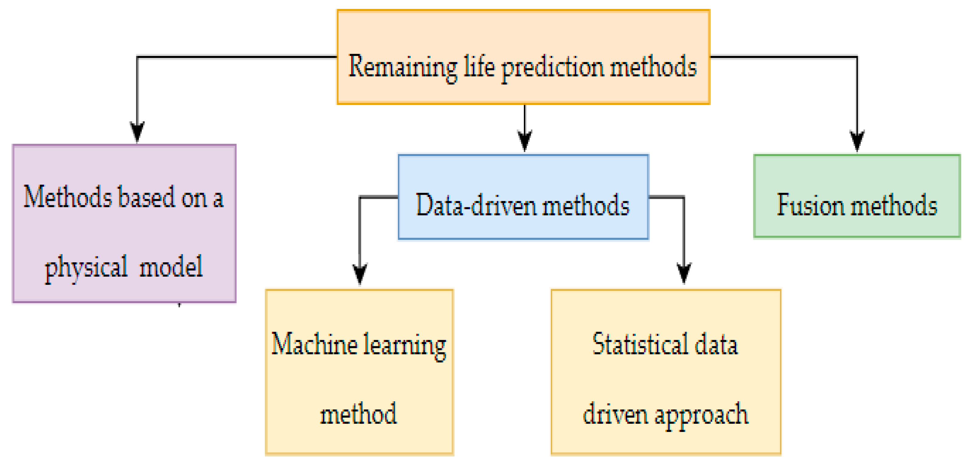
2.2.2. Data-Driven Method

  • Machine learning method
Machine learning makes a computer simulate human learning behavior and continuously trains the model by obtaining new information to improve the generalization ability of the model [54]. Due to the powerful data processing ability of machine learning, this method is widely used in data mining, speech recognition, computer vision, fault diagnosis and life prediction. According to the depth of learning, machine learning methods can be divided into traditional machine learning and deep learning methods, as shown in Figure 3. Traditional machine learning algorithms largely rely on expert prior knowledge and signal processing technology, which is difficult to automatically process and for analysis of massive monitoring data. Deep learning is developed from the traditional machine learning algorithm. With its powerful feature extraction ability, it provides a solution for training massive data and opens up a new direction for the field of machine learning [55].
(1)
Traditional machine learning methods
The methods based on traditional machine learning mainly include the methods based on neural network and support vector machine (SVM). The characteristics of each method are given in Table 5.
a
Neural network
As a mathematical processing method to simulate the structure and function of biological nervous systems, a neural network has the ability of automatic learning and summary. It mainly includes an input layer, hidden layer and output layer, which are often used to solve problems such as classification and regression [56]. After years of research and exploration, it has shown strong advantages in the field of remaining life prediction. The remaining life prediction method based on a neural network aims to take the original measurement data or the features extracted based on the original measurement data as the input of the neural network, continuously adjust the structure and parameters of the network through a certain training algorithm, and use the optimized network to predict the residual life of the equipment online. The prediction process does not need any prior information and is completely based on the prediction results obtained from the monitoring data [57]. At present, the methods based on a neural network mainly include the methods based on a multi-layer perceptrons (MLP) neural network, the methods based on a radial basis function (RBF) neural network and the methods based on extreme learning machines (ELMS).
  • Multilayer perceptron neural network
Multilayer perceptron neural network (MLP) is a kind of feedforward neural network with a hidden layer, and the neuron model of the hidden layer and output layer is consistent. MLP is mostly trained by back propagation (BP) algorithm. In addition to using BP algorithm to train MLP, other methods are also used for training, such as in [58]. Bezazi et al. [59] used MLP artificial neural network to model the composite structure monitoring data, and trained the network through maximum likelihood estimation and Bayesian reasoning. The results showed that the network has good generalization ability. On this basis, Pierce et al. [60] further analyzed the robustness of the network based on interval uncertainty technology. This kind of research provides another idea for MLP-based neural network training.
Because MLP has the ability to approximate any form of nonlinear function by adding hidden layers or hidden elements, it has attracted extensive attention in the field of remaining life prediction.
  • Radial basis function neural network
Radial basis function neural network (RBF) neural network is a neural network structure proposed in the 1980s. It has a three-layer feedforward network with a single hidden layer, and can approach any continuous nonlinear function with any accuracy [61,62]. The biggest difference between RBF neural network and MLP neural network in structure is that the independent variable of excitation function is the product of distance and deviation between input vector and weight vector, rather than the weighted sum between input vector and weight vector. Liu et al. [63] pointed out that the key to an RBF neural network model is to correctly select the appropriate RBF center. The number and location of RBF centers in the hidden layer directly affect the approximation ability of the network. Li et al. [64] constructed a life prediction model of accelerated life test by using the method of grey RBF neural network. The test showed that the prediction result is obviously better than BP neural network. When Li et al. [65] used RBF neural network for relay life prediction, the input information of RBF neural network was not the original relay overtravel time with non-stationary characteristics, but the random term obtained through wavelet transform. The output information of RBF neural network realized the relay life prediction again through wavelet packet reconstruction. Chen et al. [66] proposed a multivariate grey RBF hybrid model for remaining life prediction of industrial equipment, which integrates the advantages of grey model and RBF neural network, effectively ensures the prediction accuracy and has practical engineering application value.
The remaining life prediction method based on RBF neural network only contains one hidden layer, and the fitting accuracy is high. It can overcome the problems of falling into local optimization and slow convergence of the learning process, and can realize the dynamic determination of the network structure and the data center of the hidden layer unit.
  • Neural network based on limit learning machine
Limit learning machine (elms), as a new learning algorithm for a single hidden layer feedforward neural network, was proposed by Huang [67]. The basic idea of the elms training process is to randomly select the input weight and hidden layer deviation value, manually select the number of hidden layer neurons according to the engineering practice experience, and determine the output weight by the least square method, so as to realize the rapid determination of network structure and parameters.
Li et al. [68] studied the problem of remaining life prediction of fan mechanical transmission components based on elms, and introduced in detail the principle, parameter selection and optimization process of the elms algorithm, so as to predict the trend and value of relevant performance parameters and realize the evaluation of performance parameters and the prediction of residual life. Liu et al. [69] extracted the features that can better reflect the bearing degradation process through the joint approximate diagonalization method of the two-layer feature matrix, and input the extracted features into the elms model to accurately predict the remaining life of the bearing. On this basis, Liu et al. [70] improved the feature extraction method, also used the elms method to train the extracted features, and applied this method to the study of the remaining life of bearings. Du et al. [71] proposed a multi classification probability elms model based on sigmoid a posteriori probability mapping and Lagrange pairwise coupling method, which solved the problem of remaining life prediction of UAV transmitters. Yang et al. [72] proposed a remaining life prediction method based on elms, compared the relationship and difference between elms and BP artificial neural network, and found that the internal parameters of elms do not need iterative calculation. The test showed that the model based on elms is slightly inferior to the model based on BP artificial neural network in prediction accuracy and stability, but can significantly reduce the training time.
The remaining life prediction method based on elms has the following advantages: It can make a rapid remaining life prediction and effectively reduce the model training time. The activation function can use discontinuous functions. The problem of sensitive selection of learning parameters and easily falling into local extremum in gradient descent learning algorithm is avoided.
Although the method based on elms has many advantages, it also has some shortcomings. Since the deviation between the input weight and the hidden layer is generated randomly, the network training effect of elms cannot be guaranteed, which may be good and bad from time to time. At the same time, the number of hidden layer nodes needs to be selected according to experience and experimental methods, which makes it difficult to ensure the optimal model. In addition, because the output weight is calculated by the least square method, the method based on elms will face the problem of expanding the influence of outliers and noise.
b
Method based on support vector machine
Support vector machine (SVM) was developed based on VC dimension theory and the structural risk minimization principle. It was first proposed by Cortes and Vapnik in 1995. It is mainly used to solve the classification and regression problems of ML and is suitable for analyzing small samples and multidimensional data [73,74].
The main idea of the research on the remaining life prediction method based on SVM is to train the support vector machine model with the condition monitoring data obtained in the actual project, determine the model parameters (insensitivity coefficient, penalty factor, kernel function parameters, etc.), predict the future state of the system based on the trained SVM model, and obtain the residual life of the equipment by comparing with the preset failure threshold.
Due to the multidimensional, nonlinear and uncertain characteristics of condition monitoring data in practical engineering, it is usually difficult to ensure the accuracy of SVM model parameters by simply using a SVM method to train condition monitoring data. SVM model parameters directly affect the remaining life results of equipment. Therefore, scholars began to pay attention to how to combine SVM with other methods to predict the remaining life of equipment.
In order to eliminate the interference information in the data, Miao et al. [75] combined wavelet analysis with SVM to predict the remaining life of a gyroscope. Nieto et al. [76] proposed an algorithm based on Hybrid Particle Swarm Optimization and SVM for spacecraft engine remaining life prediction, solved the optimization problem of super parameters in the training process of support vector machine, and further improved the accuracy of prediction. Aiming at the problem that SVM cannot effectively deal with non-static sequences with monotonic trends, Maior et al. [77] proposed a method combining empirical mode decomposition and SVM for degradation data analysis and remaining life prediction, and applied the proposed method to the analysis of a motor. The results showed that this method can improve the prediction performance compared with simple SVM.
The remaining life prediction method based on SVM is more suitable for analyzing small samples and multidimensional data. However, there are also many defects. For example, with the increase in the sample set, the linearity will increase, resulting in the increase of overfitting and calculation time. It is difficult to obtain the prediction of probability formula, that is, it is impossible to evaluate the uncertainty of remaining life prediction; the Kernel function must satisfy the Mercer condition.
Table 5. Classification and characteristics of traditional machine learning remaining life prediction methods.
Traditional Machine Learning Remaining Life Prediction MethodAdvantagesDisadvantages
Neural networkMLPHas the ability to approximate any form of nonlinear function by adding hidden layers or hidden elements [60].The effect is good without obvious disadvantages [60].
RBFThe network contains only one hidden layer, and the fitting accuracy is high; It can overcome falling into local optimization and realize the dynamic determination of the network structure and the data center of the hidden layer unit [61,62].The effect is good without obvious disadvantages [66].
ELMShort training time; The activation function can use discontinuous functions; It avoids the problems of sensitive selection of learning parameters and easily falling into local extremum [67].Since the deviation between the input weight and the hidden layer is generated randomly, the network training effect of elms cannot be guaranteed, which may be good and bad from time to time. The number of hidden layer nodes needs to be selected according to experience and experimental methods, which makes it difficult to ensure the optimal model [72].
SVMThe remaining life prediction method based on SVM is more suitable for analyzing small samples and multidimensional data [75].With the increase of the sample set, the linearity will increase, resulting in the increase of overfitting and calculation time. It is difficult to obtain the prediction of probability formula, that is, it is impossible to evaluate the uncertainty of remaining life prediction; the Kernel function must satisfy the Mercer condition [77].
(2)
Deep learning
The research on equipment remaining life prediction methods based on deep learning mainly include: methods based on deep neural network (DNN), methods based on deep belief network (DBN), methods based on convolutional neural network (CNN) and methods based on recurrent neural network (RNN). The characteristics of each method are given in Table 6.
  • Deep neural network
Deep neural network (DNN) is usually a multilayer neural network formed by stacking multilayer feature representation models. The common feature representation models include AE and denoising automatic encoder (DAE). The main idea of the method based on DNN is to extract the high-level features of the original data through multiple AE or DAE stacking networks, and then realize the prediction of the remaining life based on regression fitting method or feedforward neural network. Zhou et al. [78] proposed an early diagnosis method of micro, slowly varying faults based on DNN. The high-dimensional fault features extracted by deep learning are transformed into one-dimensional fault features through the PCA method, and then the life prediction model is constructed by using the nonlinear fitting method. Yan et al. [79] studied a remaining life prediction method combining deep DAE and regression analysis for the big data analysis of industrial systems. Two deep DAEs were used to process the far end signal and near end signal, respectively to obtain the overall trend and current change process. The outputs of the two deep DAEs were fused to predict the residual life of the equipment through linear regression.
The DNN prediction method has the following characteristics: Useful features can be extracted through multiple dimensionality reduction of input data, which can facilitate model training. Because the DAE has the function of noise reduction and filtering, the network formed by the stacking of multiple DAEs can process the monitoring data containing noise, which fully reflects the strong robustness and universality of this method.
  • Deep belief network
As a typical deep learning method, DBN is mainly a deep network composed of multiple restricted Boltzman machines (RBM) stacked and a classification layer or regression layer. It can not only realize the feature representation and extraction of observation data from low-level to high-level, but also discover the distributed features of input data [80]. Deutsch et al. [81] successfully applied DBN to predict the remaining life of bearings, but the prediction accuracy of the proposed method was much lower than that of the particle filter method. Deutsch et al. [82] also proposed a remaining life prediction method for rotating equipment integrating DBN and a feedforward neural network (FNN), which is based on the improvement and expansion of the DBN method and can effectively combine the feature extraction ability of DBN with the prediction performance of FNN.
In order to obtain the probability distribution of remaining life, DBN and particle filter have been effectively combined to further improve the prediction accuracy [83]. On this basis, Zhao et al. [84] effectively combined the advantages of DBN and RVM to study a new method for predicting the remaining life of Li batteries. Because DBN has strong feature extraction ability, it effectively solves the uncertainty problem caused by artificial feature extraction and selection, and realizes the goal of intelligent feature extraction. At the same time, the time-domain signal under this method does not need to meet the requirements of periodicity, so it has a broad application space in the field of remaining life prediction.
However, DBN still has several limitations: The short-term prediction performance is good, while the long-term prediction performance is poor. It cannot reflect the uncertainty of the prediction results. Generally, it needs to be combined with other methods to reflect the uncertainty of the prediction results.
  • Convolutional neural network
As a kind of classical feedforward neural network, CNN was first proposed by Lecun and was used to solve the problem of image processing. It is mainly composed of several convolution layers and pooling layers. The purpose is to extract the topology features hidden in the monitoring data step by step by constructing multiple filters, and the extracted features will become more and more abstract with the deepening of the network level [85]. For CNN, the convolution layer uses the original input data to convolute multiple local filters, and the subsequent pooling layer can extract the most important features with a fixed length. The commonly used pooling function is the maximum pooling function [86].
The research on remaining life prediction based on CNN began in 2016. Babu et al. [87] applied deep CNN to the field of remaining life prediction, used two convolution layers and two pooling layers to extract the characteristics of the original signal, and combined with MLP to predict the remaining life. Li et al. [88] proposed a multivariable equipment residual life estimation method based on deep CNN. In order to better extract features, the time window method is used to obtain samples. At the same time, because some effective information will be filtered out by the pooling operation, the pooling layer is ignored in the process of building the network. Ren et al. [89] studied the problem of bearing remaining life prediction based on CNN, combined a series of extracted features, namely the spectrum main energy vector, into a feature map, and extracted a one-dimensional vector that is helpful for predicting the remaining life through the structure of CNN. The one-dimensional vector is input into the deep neural network to predict the residual life. The bearing test showed that the proposed method is better than the traditional ML method.
The research on remaining life prediction based on CNN has the following characteristics: It is suitable for engineering equipment that can monitor massive data. It can realize automatic feature extraction and recognition without manual participation and intervention. The weight-sharing feature makes the number of parameters of CNN model less and the optimization process more convenient. However, the remaining life prediction based on CNN is still in the preliminary exploration stage, the research results have not been systematic, and the uncertainty of remaining life cannot be given quantitatively. Therefore, the methods based on CNN still require in-depth research.
  • Recurrent neural network
RNN is a kind of feedforward neural network including a feedforward connection and an internal feedback connection, and is mainly used to process the monitoring vector sequence with interdependent characteristics. Due to its special network structure, it can retain the state information at the last moment on the hidden layer, so it has strong advantages in the field of complex dynamic system modeling [90].
The basic idea of remaining life prediction methods based on RNN is to take the monitoring data input in the project as the input of the RNN network, and train the model parameters through back propagation through time (BPTT), so as to realize the remaining life prediction of equipment. It should be noted that the internal feedback connection of an RNN depicts the pre- and post-dependence of monitoring data. Liu et al. [91] used an adaptive RNN to predict the remaining life of Li batteries, and online optimized the weight of the network structure through a cyclic Levenberg–Marquardt method. The remaining life prediction method based on RNN can integrate the original learning samples with the new learning mode to realize the retraining of samples. It can not only improve the accuracy of remaining life prediction, but also has the characteristics of fast convergence and high stability. However, the traditional RNN usually has the problem of “memory decay”, because there is no structure to control memory flow in the traditional circulation layer. When dealing with long-term dependent degradation data, the traditional RNN methods will face the problem of gradient disappearance or explosion, and the prediction accuracy will be seriously affected. On the other hand, RNN cannot effectively analyze and process multidimensional data, and usually needs to be combined with other methods for these purposes.
Scholars have also proposed other improved deep learning methods to predict the RUL, which show better performance than the current popular models. For instance, Zhang et al. [91] proposed a dual-task network structure based on bidirectional gated recurrent unit (BiGRU) and multigate mixture-of-experts (MMoE), which simultaneously evaluates the health state and predict the RUL of industrial equipment.
Table 6. Classification and characteristics of deep learning remaining life prediction methods.
Deep Learning MethodAdvantagesDisadvantages
DNNModel training is convenient; It can process the monitoring data containing noise, which shows that the method has strong robustness and universality [78].The effect is good without obvious disadvantages [79].
DBNDBN has strong feature extraction ability [80].The short-term prediction performance is good, while the long-term prediction performance is poor; It cannot reflect the uncertainty of the prediction results [84].
CNNIt is applicable to engineering equipment that can monitor massive data; It can realize automatic feature extraction and recognition without manual participation and intervention; The weight-sharing feature makes the number of parameters of a CNN model less and the optimization process more convenient [85].It is still in the preliminary exploration stage, and the research results have not been systematized;
The uncertainty of remaining life cannot be given quantitatively [89].
RNNIt can integrate the original learning samples with the new learning mode to realize the retraining of samples, improve the prediction accuracy, and has the characteristics of fast convergence and high stability [90].Traditional RNN usually has the problem of “memory decline”. When dealing with long-term dependent degraded data, it will face the problem of gradient disappearance or explosion, and the prediction accuracy will be affected; RNN cannot effectively analyze and process multidimensional data [92].
2.
Statistical data-driven approach
The statistical data-driven method is based on the theory of probability statistics, using the historical data degradation trajectory of similar systems or products, establishing the relationship between the data system and the degradation model, and estimating the parameters of the degradation model, so as to obtain the analytical probability distribution of the remaining life of the object or system and realize the prediction of the remaining life [93].
Statistical data-driven methods assume that the degradation model is known in advance, and directly use the condition monitoring data or environmental data to estimate the model parameters offline or online. However, the degradation model in practical engineering is unknown, and the degradation models of different types of equipment are different. The improper selection of a degradation model will seriously affect the prediction accuracy of remaining life. Typical methods include Wiener process, gamma process, inverse Gaussian process, Markov model and so on (see Table 7).
  • Wiener process
The method based on the Wiener process is mainly applicable to the non-monotonic case of equipment performance degradation process. This method mainly uses the following mathematical model to describe the degradation process:
X ( t ) = x 0 + 0 t λ ( s ) d s + σ B ( t )
where x0 is the initial performance degradation value; λ(s) is the drift parameter; σ is the diffusion coefficient; B(t) is the standard Brownian motion.
After obtaining the equipment performance degradation process model, the remaining life distribution of the equipment can be calculated by using the relevant theory of the Wiener process on the basis of giving its failure value. In order to realize the accurate real-time prediction of the remaining life of the equipment, usually, the real-time monitoring information of the equipment can be used to dynamically update the remaining life prediction results. Gebraeel et al. [94] first established the degradation model of equipment based on the Wiener process with linear drift (or linearization), and assumed that the drift coefficient obeyed the normal distribution. According to the degradation data observed in real time, the online update of the random drift coefficient was realized by using the method of Bayesian reasoning. The Gebraeel method has had a great impact in the field of equipment life prediction and health management. However, the remaining life prediction results obtained by the Gebraeel method are only applicable to linear degradation equipment or equipment whose performance degradation data can be directly linearized. Moreover, the Brownian motion term in the degradation model used in this method is only treated as the observation error, so that the remaining life distribution obtained is not the exact solution in the sense of first arrival time.
  • Gamma process
The gamma process is often used to model the degradation trajectory of monotonic data, such as metal wear and crack growth. Abdel et al. [95] first proposed it in 1975 and used the gamma process to model continuous monotonic degradation data. Bagdonavicius considered the influence of dynamic environments in the degradation model and proposed a remaining life prediction method based on the gamma process considering dynamic environments [96]. Lawless et al. [97] considered the problem that the parameters in the gamma process are random variables. In practical application, the duty cycle of the system may not be periodic, which would lead to aperiodic degradation measurements. Both of these factors affect the accuracy of health assessment and RUL prediction. In order to meet these challenges, Zhao et al. [98] propose a Gamma state-space model of power equipment, which considers the temporal uncertainty, measurement uncertainty, and device-to-device heterogeneity. This method introduces a new idea for health assessment and RUL prediction.
  • Inverse Gaussian process
The basic idea of the inverse Gaussian process is to assume that the degradation is strictly monotonic, and the increment of degradation obeys an inverse Gaussian distribution. The degradation process is described by the change in increment. The inverse Gaussian process was first proposed by Wasan et al. [99] in 1968, but it was not applied to the degradation modeling of equipment by Wang et al. [100] until 2010. The inverse Gaussian process is used to describe the monotonic degradation process due to the connection between the inverse Gaussian distribution and the linear drift Wiener process. Compared with the gamma process, the inverse Gaussian process is easier to deduce and implement mathematically, and more flexible and applicable.
  • Markov model
The Markov chain method is often used in the degradation modeling of processes with continuous time discrete state characteristics. This method is based on two assumptions: one is that the future degradation state is only determined by the current degradation state, that is, it is memoryless. Second, the system monitoring data can reflect its working state. The remaining life prediction method based on Markov chain defines the first arrival time by the time when the degradation process first reaches the failure state, and calculates the remaining life according to the first arrival time. Kharoufeh et al. [101] carried out a series of studies on this method and proposed a degradation model based on Markov chain considering environmental impact. Lee et al. [102] incorporated a Markov property in the degradation process into remaining life prediction based on a regression model.
Table 7. Classification and characteristics of statistical data-driven remaining life prediction methods.
Statistical Data-Driven Remaining Life Prediction MethodCharacteristics
Wiener processIt is applicable to the non-monotonic situation of equipment performance degradation process [94].
Gamma processDegradation trajectory modeling commonly used for monotone data [98].
Inverse GaussianAssuming that the degradation is strictly monotonic, and the increment of degradation obeys an inverse Gaussian distribution, the degradation process is described by the change in increment [100].
MarkovDegradation modeling for processes with continuous time discrete state characteristics [102].

3. Accuracy Evaluation Methods

3.1. Regression Index

The formula of mean absolute error (MAE) is [103]:
M A E = 1 N i = 1 N | y i - y ^ i |
where N is the number of samples, yi is the real value of the ith sample, y ^ i is the predicted value of the ith sample, y ¯ i is the average value of the sample data.
The mean square error (MSE) formula is [104]:
M S E = 1 N i = 1 N ( y i - y ^ i ) 2
The formula of mean absolute percentage error (MAPE) is [105]:
M A P E = 100 N i = 1 N | y i - y ^ i y i |
MAPE expresses the prediction effect by calculating the absolute error percentage. The smaller the value, the better. If MAPE equals 10, this indicates that the predicted average deviates from the true value by 10%.
Since MAPE calculation is independent of dimension, different problems are comparable in specific scenarios. However, the disadvantages of MAPE are also obvious, and there is no definition at yi = 0. In addition, it should be noted that the penalty of MAPE for negative error is greater than that for positive error.
The formula of root mean square error (RMSE) is [106]:
R M S E = 1 N i = 1 N ( y i - y ^ i ) 2
RMSE represents the sample standard deviation of the difference between the predicted value and the real value. Compared with MAE, RMSE has a greater penalty for large error samples. However, one disadvantage of RMSE is that it is sensitive to outliers, which will lead to very large RMSE results.
Based on RMSE, there is also a commonly used variant evaluation index called root mean square logarithmic error (RMSLE), the formula of which is:
R M S L E = 1 N i = 1 N ( log ( y i + 1 ) - log ( y ^ i + 1 ) ) 2
RMSLE penalizes the samples with small predicted value more than those with large predicted value.
The determination coefficient is mainly evaluated by (R-square) [107], and the formula is:
R S q u a r e = 1 i = 1 N ( y i y ^ i ) 2 i = 1 N ( y i y ¯ i ) 2
R-square is used to measure the proportion of the variation of dependent variables that can be explained by independent variables. The general value range is 0~1. The closer R-square is to 1, the greater the proportion of the sum of regression squares in the total sum of squares, the closer the regression line is to each observation point, the more the variation in y value is explained by the change in x, and the better the fitting degree of regression.

3.2. Classification Index

TP, TN, FP and FN are mainly used to count the problems of two categories [108]. Of course, multiple categories can also be counted separately, and the samples can be divided into positive samples and negative samples (see Table 8).
The first letter in TP, TN, FP and FN indicates whether the recognition result of the classifier is correct. The first letter of true is t, and the first letter of false is f. The second letter indicates the decision result of the classifier; P indicates that the classifier decides to be a positive sample, and N indicates that the classifier decides to be a negative sample. TP: the classifier recognizes correctly, and the classifier considers the sample as a positive sample; TN: the classifier recognizes correctly, and the classifier considers the sample as a negative sample; FP: the recognition result of the classifier is wrong, and the classifier thinks the sample is a positive sample, therefore, in fact, the sample is a negative sample; FN: the recognition result of the classifier is wrong, and the classifier considers the sample to be a negative sample, therefore, in fact, the sample is a positive sample.
Accuracy refers to the proportion of the number of samples with correct model prediction (including true prediction and false prediction) in the total number of samples [109], i.e.,
A c c u r a c y = m c o r r e c t m t o t a l
where mcorrect represents the number of samples correctly classified by the model, and mtotal represents the number of all samples.
Accuracy is one of the simplest and most intuitive evaluation indicators in classification problems, but there are some limitations in accuracy. For example, in the second classification, when negative samples account for 99%, if the model predicts all samples as negative samples, it can also obtain 99% accuracy [110]. Although the accuracy seems high, this model is actually useless because it cannot find a positive sample.
Precision refers to the proportion of the number of samples predicted to be true by the model and actually true to the number of samples predicted to be true by the model [111], i.e.,
P r e c i s i o n = T P T P + F P
Recall refers to the proportion of the number of samples predicted by the model and actually true to the number of samples actually true [112], i.e.,
R e c a l l = T P T P + F N
Generally speaking, the accuracy rate and recall rate are mutually exclusive; that is to say, if the accuracy rate is high, the recall rate will become low. If the recall rate is high, the accuracy rate will be low. Therefore, an index value considering both accuracy and recall is designed. The value is the harmonic average of accuracy rate and recall rate [113], i.e.,
F 1 = 2 P r e c i s i o n R e c a l l P r e c i s i o n + R e c a l l
In some scenarios, we pay different attention to the accuracy rate and recall rate. At this time, the Fa value in the more general form of F1 value can be satisfied. The Fa value is defined as follows:
F α = ( 1 + α ) P r e c i s i o n R e c a l l α 2 P r e c i s i o n + R e c a l l
We average all the arithmetic indexes in [114], and then calculate the average value of each category.
P r e c i s i o n m a c r o = i = 1 N Pr e c i s i o n i
R e c a l l m a c r o = i = 1 N R e c a l l i
F α - m a c r o = ( 1 + α ) P r e c i s i o n m a c r o R e c a l l m a c r o α 2 P r e c i s i o n m a c r o + R e c a l l m a c r o
where i represents the ith category.
We establish a statistical matrix for each instance, and then calculate the corresponding data in the global index set [115].
P r e c i s i o n m i c r o = T P ¯ T P ¯ + F P ¯
R e c a l l m i c r o = T P ¯ T P ¯ + F N ¯
F α = ( 1 + α ) P r e c i s i o n m i c r o R e c a l l m i c r o α 2 P r e c i s i o n m i c r o + R e c a l l m i c r o

3.3. Index Selection Principle

If the health state grade is used to evaluate the health degree of the equipment, it can be regarded as a classification problem, and the indicators of the above classification problems can be used [116,117]. If a specific value is used to evaluate the health of the equipment, it can be regarded as a regression problem, and the indicators of the above regression problem can be used. However, the regression problem can also be transformed into a classification problem, so as to use the indicators of the classification problem.
If the regression scheme is adopted, the recommended evaluation index is mean square error or R-square. If the classification scheme is adopted, the recommended evaluation index is accuracy or F1 value.

4. Application of Health State Estimation and Remaining Life Prediction

4.1. Application of Health State Estimation in Various Industries

Each industry has estimated the health degree of the following products, and the specific contents are shown in the Table 9: The power industry mainly estimates the health of electronic products such as battery energy storage systems and electric energy meters, electrical products such as wind turbine drive chains and generator sets, and mechanical products such as power mechanical equipment. The transportation industry mainly evaluates the health of vehicle batteries and other electronic products. The Internet industry mainly estimates the health of electronic products such as server hosts. The petrochemical industry mainly estimates the health of electronic products such as coal mine underground systems and electrical products such as electric submersible pumps. The water industry mainly estimates the health of electrical products such as water supply equipment. The manufacturing industry mainly estimates the health of mechanical products such as robots and electrical products such as air conditioners. The medical industry mainly estimates the health of human muscles. It can be seen that health state estimation has been applied to a wide extent in industry. In addition, there are a variety of health state estimation methods.

4.2. Remaining Life Prediction in Various Industries

Each industry has made RUL predictions on certain products (see Table 10), as follows: In the aviation field, RUL prediction is carried out for electronic products such as hierarchical control systems and mechanical products such as blades. In the power industry, RUL prediction is carried out for electronic products such as power batteries, converters and power modules. In the vehicle industry, RUL prediction is made for electrical products such as mechanical relays and mechanical products such as brake shoes. In the household appliance industry, RUL prediction is made for mechanical equipment such as rolling bearings. It can be seen that remaining life prediction has been applied to a certain extent in industry, but it is not widely used compared with health state estimation. In addition, there are a variety of remaining life prediction methods used in industry.

5. Applicable Objects of the Methods

The objects of health state estimation and remaining life prediction are different. Among them, health state estimation is applicable to equipment with a high failure rate and low importance. Remaining life prediction is applicable to equipment with a low failure rate and high importance.
In the rail transit industry, the average annual failure frequency can be used as an indicator of failure rate, and the delay time can be used as an indicator of importance. Using these two indicators, the equipment of rail transit is divided into four categories. Among them, the equipment with high annual failure frequency and low delay time is suitable for health state estimation, and industrial computers constitute such equipment. The equipment with low annual failure frequency and high delay time is suitable for remaining life prediction, and the power supply is one such piece of equipment. The equipment with low annual failure frequency and low delay time is suitable for fault alarm. Subsystems and components with high annual failure frequency and delay time are suitable for design improvement.

6. Conclusions

6.1. Methods Summary

In terms of health, the following summary is given:
(1) Various health state estimation methods have been applied in industry. The health state estimation method has been applied in the industry to a certain extent, and the application objects include electronic, electrical, mechanical equipment and so on. Therefore, it is feasible to estimate the health degree of equipment in various industries.
(2) The health state estimation methods based on non-machine learning and machine learning are suitable for different objects. Among them, non-machine learning methods have the advantages of strong interpretability, being easy to understand and they do not need a lot of equipment, but they also have the disadvantages of poor generalization and subjective weight determination. Machine learning methods have the advantages of strong generalization ability, but they have the disadvantage of weak interpretability. Based on the above two points, when estimating the health of equipment, if the number of output parameters is small, the relationship between fault and output parameters can be listed, and the method needs some explanation, the non-machine learning methods are recommended. If the amount of equipment data is sufficient and the method needs strong generalization ability, and in addition, if the equipment output parameters are complex and the relationship between fault and output parameters cannot be obtained, the machine learning methods are recommended.
(3) The accuracy and reliability of health state estimation are affected by many factors. In terms of accuracy, before the implementation of the two health state estimation methods, experts need to establish the corresponding relationship between parameters and scores, that is, expert scoring, also known as expert labeling. The quality of expert scoring basically determines the upper limit of the accuracy and reliability of machine learning methods. Moreover, if the equipment data cannot cover most degradation situations in equipment engineering applications, the accuracy of health state estimation will also be affected. In addition, the assessment indicators of health state estimation effect (false report and missing report) are different, and the estimation effect is also different.
The remaining life prediction is summarized as follows:
(1) Various remaining life prediction methods are applied in industry. The application objects mainly involve electrical and mechanical equipment with obvious degradation laws. Therefore, it is feasible to predict the remaining life of equipment in various industries.
(2) The remaining life prediction methods based on a physical model and data are applicable to different objects. Among them, the physical model method is suitable for equipment with a single degradation characterization parameter and a clear degradation mechanism, but its generalization ability is poor. The machine learning methods in the data-driven methods have the advantages of strong data-driven ability and good generalization. They are suitable for equipment with multiple degradation characterization parameters, and are extremely suitable for equipment with an unclear relationship between the degradation characterization parameters and their failure. The statistical data-driven methods in the data-driven methods have strong interpretability and are suitable for equipment with only a single degradation characterization parameter and significant degradation characteristics. Based on the above three points, the physical model method is not suitable for the remaining life prediction of rail transit equipment. When predicting the residual life of equipment, if the equipment has only one degradation characterization parameter and needs some explanation, the statistical data-driven methods are recommended. If there are many equipment output parameters and the relationship between the equipment output parameters and their failure is not clear, the machine learning methods are recommended.
(3) The accuracy of remaining life prediction is greatly affected by equipment degradation data and actual working conditions of equipment. The premise of remaining life prediction is to have sufficient equipment degradation data or equipment life data as support. If the test conditions covered by the data are single and the types of working conditions are less, the representativeness of the data is poor. The remaining life prediction methods trained by the data in this case have poor accuracy and applicability. In addition, if the actual working conditions of the equipment change greatly, the general life prediction methods cannot meet the accuracy requirements, and the life prediction methods need to be improved.
The selection of accuracy evaluation methods is summarized as follows:
(1) The health state estimation methods can be classified as both s classification problem and a regression problem. The appropriate index evaluation method needs to be selected according to the specific situation. Remaining life prediction is a regression problem, which can be evaluated by regression index.
(2) The recommended classification evaluation index is accuracy or F1 value, and the recommended regression evaluation index is mean square error or R-square.

6.2. Feasibility Analysis

Feasibility analysis of health state estimation methods:
(1) The economic cost, time cost and labor cost of fault injection tests are within an affordable range. Because the training data and verification data of health state estimation methods can be derived from fault injection test, the sample of this test can be recycled, so the economic cost of the test sample is within an acceptable range. Since this test can be conducted intermittently and the time spent in each group of tests can be reduced to weeks, the test time is also within the acceptable range. In addition, the test needs the cooperation of engineers who are proficient in products, data acquisition and accelerated life tests. If there are engineers with these abilities in the unit, it is feasible only from the perspective of manpower.
(2) The time cost and labor cost of exploring the health state estimation methods are large. If the company has no research foundation in this field, the exploration and comparison of various non-machine learning methods will take a long time. The labor cost depends on the number of non-machine learning health state estimation methods. If more non-machine learning health state estimation methods are selected, the labor cost will be large.
(3) The health degree estimation methods can bring greater economic benefits and better social benefits. If the equipment in the industry is more suitable for health state estimation, these health state estimation methods can be applied to a wide range of engineering in the future, which will bring great economic benefits. Engineering application can greatly improve the operation safety and reliability of unit products, so as to obtain better social benefits.
Feasibility analysis of remaining life prediction methods:
(1) The economic cost, time cost and labor cost of accelerated life test are significant. Because the training data and verification data of remaining life prediction methods need to be derived from accelerated life test, this test is a destructive test, and the sample cannot be recycled. Therefore, the economic cost of the test sample is high. Since this test needs to be carried out continuously until the sample fails, the time spent on each group of tests is basically half a year, so the test time is long. In addition, during the accelerated life test, personnel are required to be on duty 24 h a day, and engineers proficient in products, data acquisition and accelerated life test are required to work together, so the labor cost is high.
(2) The time cost and labor cost of exploring the remaining life prediction methods are large. If the unit has no previous experience in remaining life prediction methods, the exploration of various remaining life prediction methods will take a long time. The labor cost depends on the number of remaining life prediction methods utilizing machine learning. If more machine learning remaining life prediction methods are selected, the labor cost will be greater.
(3) The remaining life prediction methods can bring less economic and social benefits. If only some equipment in the unit is suitable for remaining life prediction, the engineering application volume of remaining life prediction method is poor and the economic benefits are small.

Author Contributions

J.Z. formulated the overall research objectives, carried out the research design and manuscript writing. C.G. and T.T. formulated the overall research objectives. X.X., M.L. and B.Y. made contributions to the research idea. All authors have read and agreed to the published version of the manuscript.

Funding

This work was research was funded by the National Key R&D Program of China, grant number 2020YFB1600705, and the Beijing Science and Technology Project, grant number Z191100002519003.

Data Availability Statement

All data in this study are available in the documents referenced in bibliography.

Conflicts of Interest

Authors declare that there is no conflict of interest with Traffic Control Technology Co., Ltd.

References

  1. Zeng, S.K.; Michael, G.P.; Wu, J. Current situation and development of fault prediction and health management (PHM) technology. J. Aeronaut. 2005, 26, 7–11. [Google Scholar]
  2. Xu, P.; Kang, R. Research on prediction and condition management system (PHM) technology. Meas. Control Technol. 2004, 23, 58–60. [Google Scholar]
  3. Ma, S.S.; Chen, G.S.; Fang, X.B. Preliminary study on fault prediction and health management system of complex equipment. Comput. Meas. Control 2010, 1, 8–14. [Google Scholar]
  4. Chan, Z.Q. Research on Equipment Health Assessment and Residual Life Prediction Method Based on LSTM Network; University of Science and Technology of China: Hefei, China, 2019. [Google Scholar]
  5. Zhan, L.X.; Liu, J.; Liu, C.J. A health condition evaluation method for equipment based on parameter characteristics. Electron. Prod. Reliab. Environ. Test. 2018, 4, 12–18. [Google Scholar]
  6. Ma, D.Z. Health monitoring and evaluation of large complex systems based on multi-source information fusion. High Tech. Ind. 2018, 5, 16–23. [Google Scholar]
  7. Sun, T.H. Evaluation of Equipment Health Based on D-S Evidence Theory; Xi’an Technological University: Xi’an, China, 2021. [Google Scholar]
  8. Huang, S.M.; Zhu, W.; Wang, Y.D. Reliability evaluation model of high voltage XLPE cable based on load rate and health state. Electr. Meas. Instrum. 2017, 54, 8–11. [Google Scholar]
  9. Zio, E.; Maio, F.D. A data-driven fuzzy approach for predicting the remaining useful life in dynamic failure scenarios of a nuclear system. Reliab. Eng. Syst. Saf. 2013, 95, 49–57. [Google Scholar] [CrossRef] [Green Version]
  10. Kovaevi, I.F.; Drofenik, U.; Kolar, J.W. New physical model for lifetime estimation of power modules. In Proceedings of the 2010 International Power Electronics Conference—ECCE ASIA, Sapporo, Japan, 21–24 June 2010; pp. 2106–2114. [Google Scholar]
  11. Kim, W.D.; Lee, H.J.; Kim, J.Y. Fatigue life estimation of an engine rubber mount. Int. J. Fatigue 2004, 26, 553–560. [Google Scholar] [CrossRef]
  12. Qian, Y.; Yan, R.; Gao, R.X. A multi-time scale approach to remaining useful life prediction in rolling bearing. Mech. Syst. Signal Process. 2017, 83, 549–567. [Google Scholar] [CrossRef] [Green Version]
  13. Zhan, J.; Wang, R.; Yi, L. Health Assessment Methods for Wind Turbines Based on Power Prediction and Mahalanobis Distance. Int. J. Pattern Recognit. Artif. Intell. 2019, 33, 195–206. [Google Scholar] [CrossRef]
  14. She, J.; Yao, W.; Shi, J. Multi-Dimensional Health Evaluation of Equipment in Electric Power Communication Network. In Proceedings of the IEEE 3rd Advanced Information Management, Communicates, Electronic and Automation Control Conference, Chongqing, China, 11–13 October 2019. [Google Scholar]
  15. Lv, J.W.; Yu, P.; Wei, J. Health status evaluation method of ship equipment. J. Nav. Eng. Univ. 2011, 23, 5–12. [Google Scholar]
  16. Atamuradov, V. Railway point machine prognostics based on feature fusion and health state assessment. IEEE Trans. Instrum. Meas. 2018, 32, 2691–2704. [Google Scholar] [CrossRef] [Green Version]
  17. Liu, S. A Comprehensive evaluation study on the health status of multi-feature parameters of mechanical equipment based on fuzzy hierarchical analysis. In Proceedings of the International Conference on Sensing, Diagnostics, Prognostics, and Control, Xi’an, China, 15–17 August 2018. [Google Scholar]
  18. Li, X.; Liu, Y.Y.; Li, G.H. Satellite health assessment method based on fuzzy variable weight principle. Syst. Eng. Electron. Technol. 2014, 36, 476–480. [Google Scholar]
  19. Peng, Y.L.; Li, W.G.; Liu, J. Health assessment model based on dynamic weight and fuzzy comprehensive evaluation method. Comput. Syst. Appl. 2017, 26, 37–43. [Google Scholar]
  20. Zhang, L.; Qiao, F.; Wang, J. Equipment health assessment based on improved incremental support vector data description. IEEE Trans. Syst. Man Cybern. Syst. 2019, 2, 3205–3216. [Google Scholar] [CrossRef]
  21. Xiao, J.H.; Zhao, Y.H.; Xue, X.R. Health analysis and overall operation state prediction method of electric energy meter. Power Grid Clean Energy 2016, 32, 5–11. [Google Scholar]
  22. Zhang, C.; Shu, M. Health status evaluation method based on support vector machine. Comput. Syst. Appl. 2018, 27, 9–13. [Google Scholar]
  23. Li, L.j.; Han, J.; Hao, W. Research on support vector data description for condition evaluation of mechanical equipment. Mech. Sci. Technol. 2005, 24, 4–12. [Google Scholar]
  24. Yang, S.; Meng, C.; Wang, C. Research on electronic equipment condition evaluation model based on Fuzzy SVDD. Comput. Eng. Des. 2013, 34, 5–18. [Google Scholar]
  25. Gu, M.Y.; Chen, Y.L.; Wang, X.L. Similarity life prediction method based on real-time health degree under multiple degenerate variables. Comput. Integr. Manuf. Syst. 2017, 23, 11–14. [Google Scholar]
  26. Li, S.; Zhang, G.; Jian, W. Civil aircraft health management research based on big data and deep learning technologies. In Proceedings of the IEEE International Conference on Prognostics & Health Management, Dallas, TX, USA, 19–21 June 2017. [Google Scholar]
  27. Pan, H.; Gui, G.; Lin, Z. Deep BBN learning for health assessment toward decision-making on structures under uncertainties. KSCE J. Civ. Eng. 2018, 22, 928–940. [Google Scholar] [CrossRef]
  28. Lei, Y.G.; Jia, F.; Zhou, X. Big data health monitoring method of mechanical equipment based on deep learning theory. J. Mech. Eng. 2015, 51, 8–16. [Google Scholar] [CrossRef]
  29. Li, X.; Chang, Y.; Luo, Y.; Song, B. Residual life evaluation of transformer based on health index. High Volt. Appar. 2012, 48, 80–85. [Google Scholar]
  30. Niu, G.C.; Hu, Z.; Hu, D.M. Evaluation and prediction of production line health based on matter-element information entropy. Comput. Integr. Manuf. Syst. 2019, 25, 1639–1646. [Google Scholar]
  31. Lu, F.; Huang, J.Q.; Qiu, X.J.; Xing, Y.D. Engine gas path analysis based on feature extraction by information entropy fusion. J. Instrum. 2012, 33, 13–19. [Google Scholar]
  32. Yin, A.J.; Liang, Z.X.; Zhang, B.; Wang, D.L. Bearing health evaluation method based on principal curve similarity. Vib. Test Diagn. 2019, 39, 625–630. [Google Scholar]
  33. Deng, C.; Wang, Y.H.; Wu, J.; Xia, S.; Tao, Z.K. Performance degradation modeling and health state evaluation method of electromechanical equipment. Comput. Integr. Manuf. Syst. 2018, 24, 2279–2287. [Google Scholar]
  34. Zhang, Y.; Han, G.W.; Lu, N.Y. Health status evaluation method of rail vehicle door system based on JS divergence. Mech. Des. Manuf. Eng. 2017, 46, 6–11. [Google Scholar]
  35. Bai, X.; An, Z.; Hou, Y. Health assessment and management of wind turbine blade based on the fatigue test data. In Proceedings of the Prognostics and System Health Management Conference, Chengdu, China, 19–21 October 2016. [Google Scholar]
  36. Cao, Z.H.; Shen, J.H. Sensor health evaluation method based on fuzzy set theory. J. Electr. Mach. Control 2010, 14, 6–12. [Google Scholar]
  37. Qian, H.; Zheng, S.; Zhu, P.C. Research on variable weight fuzzy health evaluation method of condenser in nuclear power plant. J. Shanghai Electr. Power Inst. 2019, 35, 8–15. [Google Scholar]
  38. Yin, M.; Ye, X.h.; Li, Q.M. Radar transmitter health assessment based on evidence fusion. J. Nav. Eng. Univ. 2015, 27, 4–12. [Google Scholar]
  39. Zhong, Z.W.; Chen, J.Y.; Tang, T. Turnout fault detection and health assessment method based on SVDD. J. Southwest Jiaotong Univ. 2018, 53, 8–15. [Google Scholar]
  40. Wagshum, A.; Wang, Y.F.; Weldegiorgis, B.H. Rotating machinery prognostics and application of machine learning algorithms: Use of deep learning with similarity index measure for health status prediction. In Proceedings of the Annual Conference of the Prognostics and Health Management Society, Philadelphia, PA, USA, 11–13 June 2018. [Google Scholar]
  41. Gu, J.X.; Wang, Z.H.; Jason, K.B.; Ma, L.Y.; Shahroudy, A.; Shuai, B.; Liu, T.; Wang, X.; Wang, G.; Cai, J.F. Recent advances in convolutional neural networks. Pattern Reg. 2018, 77, 354–377. [Google Scholar] [CrossRef] [Green Version]
  42. Liu, W.T.; Huang, Z.H.; Pan, Q.Q.; Zhang, T.; Huang, X.Y. Research on construction path of turnout health evaluation method and evaluation system based on artificial intelligence. Res. Urban Rail Transit 2020, 23, 149–153. [Google Scholar]
  43. Peng, X.Y. Data Driven Fault Prediction; Harbin Institute of Technology Press: Harbin, China, 2016. [Google Scholar]
  44. Peng, D.; Liu, Z.; Wang, H.; Qin, Y.; Jia, L. A novel deeper one-dimensional CNN with residual learning for fault diagnosis of wheelset bearings in high-speed trains. IEEE Access 2019, 7, 278–293. [Google Scholar] [CrossRef]
  45. Wu, K.; Sun, J.; Jiang, B. Research on health status evaluation method of wind tunnel equipment based on LSTM. Comput. Meas. Control 2018, 26, 288–291. [Google Scholar]
  46. Heng, A.; Zhang, S.; Tan, A. Rotating machinery prognostics: State of the art, challenges and opportunities. Mech. Syst. Signal Process. 2009, 23, 724–739. [Google Scholar] [CrossRef]
  47. Liu, D.; Wang, H.; Peng, Y.; Xie, W.; Liao, H. Satellite lithium-ion battery remaining cycle life prediction with novel indirect health indicator extraction. Energies 2013, 6, 3654–3668. [Google Scholar] [CrossRef]
  48. Pecht, M. Prognostics and Health Management of Electronics; John Wiley and Sons, Ltd.: Hoboken, NJ, USA, 2008. [Google Scholar]
  49. Li, C.J.; Lee, H. Gear fatigue crack prognosis using embedded model, gear dynamic model and fracture mechanics. Mech. Syst. Signal Process. 2005, 19, 836–846. [Google Scholar] [CrossRef]
  50. Fan, J.J.; Yung, K.C.; Pecht, M. Physics-of-failure-based prognostics and health management for high-power white light-emitting diode lighting. IEEE Trans. Device Mater. Reliab. 2011, 11, 407–416. [Google Scholar] [CrossRef]
  51. Lee, M.Y.; Tang, J. A modified EM-algorithm for estimating the parameters of inverse Gaussian distribution based on time censored Wiener degradation data. Stat. Sin. 2007, 17, 873–893. [Google Scholar]
  52. Tanaka, K.; Mura, T. A dislocation model for fatigue crack initiation. J. Appl. Mech. 1981, 48, 97–103. [Google Scholar] [CrossRef]
  53. Mou, Y.W.; Lu, S. Numerical simulation of fatigue crack initiation life of turbine disk based on material micro characteristics. J. Aeronaut. 2013, 34, 282–290. [Google Scholar]
  54. Mitchell, T.M.; Carbonell, J.G.; Michalski, R.S. Machine Learning; China Machine Press: Beijing, China, 2003; pp. 154–196. [Google Scholar]
  55. Bengio, S.; Deng, L.; Larochelle, H. Guest editors’ introduction: Special section on learning deep architectures. IEEE Trans. Pattern Anal. Mach. Intell. 2013, 35, 1795–1797. [Google Scholar] [CrossRef] [PubMed]
  56. Simon, H. Neural Network: A Comprehensive Foundation; Prentice Hall PTR: Prentice, NJ, USA, 1994; pp. 74–79. [Google Scholar]
  57. Byington, C.S.; Watson, M.; Edwards, D. Data-driven neural network methodology to remaining life predictions for aircraft actuator components. In Proceedings of the IEEE Aerospace Conference Proceedings, Big Sky, MT, USA, 6–13 March 2004. [Google Scholar]
  58. Tian, Z.G.; Wong, L.; Safaei, N. A neural network approach for remaining useful life prediction utilizing both failure and suspension histories. Mech. Syst. Signal Process. 2010, 24, 1542–1555. [Google Scholar] [CrossRef]
  59. Bezazi, A.; Pierce, S.G.; Worden, K. Fatigue life prediction of sandwich composite materials under flexural tests using a Bayesian trained artificial neural network. Int. J. Fatigue 2007, 29, 738–747. [Google Scholar] [CrossRef]
  60. Pierce, S.G.; Worden, K.; Bezazi, A. Uncertainty analysis of a neural network used for fatigue lifetime prediction. Mech. Syst. Signal Process. 2008, 22, 1395–1411. [Google Scholar] [CrossRef]
  61. Powell, M.J. Radial basis functions for multivariable interpolation:A review. Algorithms Approx. 1987, 6, 143–167. [Google Scholar]
  62. Bors, A.G. Introduction of the Radial Basis Function Networks. Electron. Eng. 1996, 13, 393–408. [Google Scholar]
  63. Liu, H.; Fan, M.J.; Zeng, Q.H. RBF network based on artificial immune algorithm and application of predicting the residual life of injecting water pipeline. Nat. Comput. 2010, 3, 1305–1309. [Google Scholar]
  64. Li, S.Z.; Li, X.Y.; Jiang, T.M. A prediction method of life and reliability for CSALT using Grey RBF neural networks. In Proceedings of the International Conference on Industrial Engineering and Engineering Management, Beijing, China, 21–23 October 2009. [Google Scholar]
  65. Li, Z.G.; Liu, B.Y.; Li, L.L. Relay life prediction based on wavelet packet transform and RBF neural network. J. Electrotech. 2015, 30, 233–240. [Google Scholar]
  66. Chen, X.S.; Xiao, H.; Guo, Y.J. A multivariate grey RBF hybrid model for residual useful life prediction of industrial equipment based on state data. Int. J. Wirel. Mob. Comput. 2016, 10, 90–96. [Google Scholar] [CrossRef]
  67. Huang, G.B.; Zhu, Q.Y.; Siew, C.K. Extreme learning machine: A new learning scheme of feed forward neural networks. In Proceedings of the IEEE International Joint Conference on Neural Networks, Budapest, Hungary, 17 January 2005. [Google Scholar]
  68. Li, L. Research on Residual Life Prediction of Fan Mechanical Transmission Components Based on Limit Learning Machine; Yanshan University: Qinhuangdao, China, 2015. [Google Scholar]
  69. Liu, F.; Liu, Y.B.; Chen, F.L. Residual life prediction for ball bearings based on joint approximate diagonalization of eigen matrices and extreme learning machine. Proc. Inst. Mech. Eng. Part C J. Mech. Eng. Sci. 2017, 231, 1–13. [Google Scholar] [CrossRef]
  70. Liu, Y.B.; He, B.; Liu, F. Remaining useful life prediction of rolling bearings using PSR, JADE, and extreme learning machine. Math. Probl. Eng. 2016, 5, 8623530. [Google Scholar] [CrossRef] [Green Version]
  71. Du, Z.L.; Li, X.M.; Xi, L.P. Multi classification probability limit learning machine and its application in remaining service life prediction. Syst. Eng. Electron. Technol. 2015, 37, 2777–2784. [Google Scholar]
  72. Yang, Z.; Baraldi, P.; Zio, E. A comparison between extreme learning machine and artificial neural network for remaining useful life prediction. In Proceedings of the Prognostics and System Health Management Conference, Chengdu, China, 19–21 October 2016. [Google Scholar]
  73. Joachims, T. Making large-scale SVM learning practical. Tech. Rep. 1998, 8, 499–526. [Google Scholar]
  74. Cherkassky, V.; Ma, Y. Practical selection of SVM parameters and noise estimation for SVM regression. Neural Netw. 2004, 17, 113–126. [Google Scholar] [CrossRef] [Green Version]
  75. Miao, J.Q.; Li, X.G.; Ye, J.H. Predicting research of mechanical gyroscope life based on wavelet support vector. In Proceedings of the First International Conference on Reliability Systems Engineering, Beijing, China, 21–23 October 2015. [Google Scholar]
  76. Nieto, P.J.G.; García-Gonzalo, E.; Lasheras, F.S. Hybrid PSO-SVM-based method for forecasting of the remaining useful life for aircraft engines and evaluation of its reliability. Reliab. Eng. Syst. Saf. 2015, 138, 219–231. [Google Scholar] [CrossRef]
  77. Maior, C.B.S.; Moura, M.D.; Lins, I.D. Remaining useful life estimation by empirical mode decomposition and support vector machine. IEEE Lat. Am. Trans. 2016, 14, 4603–4610. [Google Scholar] [CrossRef]
  78. Zhou, F.; Gao, Y.L.; Wang, J.Y. Early diagnosis and life prediction of slowly varying fault based on deep learning. J. Shandong Univ. 2017, 47, 30–37. [Google Scholar]
  79. Yan, H.; Wan, J.; Zhang, C. Industrial big data analytics for prediction of remaining useful life based on deep learning. IEEE Access 2018, 6, 17190–17197. [Google Scholar] [CrossRef]
  80. Fischer, A.; Igel, C. Progress in Pattern Recognition, Image Analysis, Computer Vision, and Applications; Springer: Berlin/Heidelberg, Germany, 2012; pp. 154–196. [Google Scholar]
  81. Deutsch, J.; He, D. Using deep learning based approaches for bearing remaining useful life prediction. In Proceedings of the Annual Conference of the Prognostics and Health Management Society, Nanjing, China, 14 July 2016. [Google Scholar]
  82. Deutsch, J.; He, D. Using deep learning-based approach to predict remaining useful life of rotating components. IEEE Trans. Syst. Man Cybern. Syst. 2017, 48, 11–20. [Google Scholar] [CrossRef]
  83. Deutsch, J.; He, M.; He, D. Remaining useful life prediction of hybrid ceramic bearings using an integrated deep learning and particle filter approach. Appl. Sci. 2017, 7, 649. [Google Scholar] [CrossRef] [Green Version]
  84. Zhao, G.Q.; Zhang, G.H.; Liu, Y.F. Lithium-ion battery remaining useful life prediction with deep belief network and relevance vector machine. In Proceedings of the IEEE International Conference on Prognostics and Health Management, Dallas, TX, USA, 19–21 June 2017. [Google Scholar]
  85. Lawrence, S.; Giles, C.L.; Tsoi, A.C. Face recognition: A convolutional neural-network approach. IEEE Trans. Neural Netw. 1997, 8, 98–113. [Google Scholar] [CrossRef] [Green Version]
  86. Sun, M.L.; Song, Z.J.; Jiang, X.H. Learning pooling for convolutional neural network. Neuro Comput. 2016, 224, 96–104. [Google Scholar] [CrossRef]
  87. Babu, G.S.; Zhao, P.; Li, X.L. Database Systems for Advanced Applications; Springer: Berlin/Heidelberg, Germany, 2016; pp. 124–129. [Google Scholar]
  88. Li, X.; Ding, Q.; Sun, J.Q. Remaining useful life estimation in prognostics using deep convolution neural networks. Reliab. Eng. Syst. Saf. 2018, 172, 1–11. [Google Scholar] [CrossRef] [Green Version]
  89. Ren, L.; Sun, Y.; Wang, H. Prediction of bearing remaining useful life with deep convolution neural network. IEEE Access 2018, 6, 13041–13049. [Google Scholar] [CrossRef]
  90. Heimes, F.O. Recurrent neural networks for remaining useful life estimation. In Proceedings of the International Conference on Prognostics and Health Management, San Francisco, CA, USA, 17–20 June 2019. [Google Scholar]
  91. Zhang, Y.; Xin, Y.; Liu, Z.W.; Chi, M.; Ma, G. Health status assessment and remaining useful life prediction of aero-engine based on bigru and mmoe. Reliab. Eng. Syst. Saf. 2022, 220, 108–123. [Google Scholar] [CrossRef]
  92. Malhi, A.; Yan, R.; Gao, R.X. Prognosis of defect propagation based on recurrent neural networks. IEEE Trans. Instrum. Meas. 2011, 60, 703–711. [Google Scholar] [CrossRef]
  93. Wang, D.; Miao, Q.; Pecht, M. Prognostics of lithium-ion batteries based on relevance vectors and a conditional three-parameter capacity degradation model. J. Power Sources 2013, 239, 253–264. [Google Scholar] [CrossRef]
  94. Gebaee, N.Z.; Lawley, M.A.; Li, R. Residual-life distributions from component degradation signals: A Bayesian approach. IIE Trans. 2005, 37, 543–557. [Google Scholar]
  95. Abdel-Hameed, M. A Gammawear process. IEEE Trans. Reliab. 1975, 24, 152–153. [Google Scholar] [CrossRef]
  96. Bagdonavicius, V.; Nikulin, M.S. Estimation in degradation models with explanatory variables. Lifetime Data Anal. 2001, 7, 85–103. [Google Scholar] [CrossRef] [PubMed]
  97. Lawles, S.J.; Crowder, M. Covariates and random effect in a Camma process model with application to degradation and failure. Lifetime Data Anal. 2004, 10, 213–227. [Google Scholar] [CrossRef] [PubMed]
  98. Zhao, S.; Peng, Y.; Yang, F.; Ugur, E.; Wang, H. Health state estimation and remaining useful life prediction of power devices subject to noisy and aperiodic condition monitoring. IEEE Trans. Instrum. Meas. 2021, 70, 1–16. [Google Scholar] [CrossRef]
  99. Wasan, M.T. On an inverse Caussian process. Scand. Actuar. J. 1968, 968, 69–96. [Google Scholar] [CrossRef]
  100. Wang, X.; Xu, D. Aninverse caussian process model for degradation data. Technometrics 2010, 52, 188–197. [Google Scholar] [CrossRef]
  101. Kharoufeh, J.P.; Cox, S.M. Evaluating failure time probabilities for a Markovian wear process. Comput. Oper. Res. 2005, 32, 1131–1145. [Google Scholar] [CrossRef]
  102. Lee, M.L.T.; Whitmore, C.A.; Rosner, B.A. Threshold regression for survival data with time-varying covariates. Stat. Med. 2010, 29, 896–905. [Google Scholar] [CrossRef]
  103. Sharrow, D.J.; Clark, S.J.; Raftery, A.E. Cross-Validation Results Showing the Mean of the Distribution of Mean Absolute Error (MAE) for Three Mortality Indicators and Amongst All-Ages and Life Tables after 1000 Iterations of Cross Validation. 2014. Available online: https://figshare.com/articles/dataset/_Cross_validation_results_showing_the_mean_of_the_distribution_of_mean_absolute_error_MAE_for_three_mortality_indicators_and_amongst_all_ages_and_life_tables_after_1_000_iterations_of_cross_validation_/1034313 (accessed on 22 April 2022).
  104. Balkenius, A.; Johansson, A.J.; Balkenius, C. Mean squared error (MSE) of the Background Estimation on Artificial Bleaching Data with Different Amounts of Noise. 2015. Available online: https://figshare.com/articles/figure/_Mean_squared_error_MSE_of_the_background_estimation_on_artificial_bleaching_data_with_different_amounts_of_noise_/1438997 (accessed on 22 April 2022).
  105. Ahmar, A.S. Forecast Error Calculation with Mean Squared Error (MSE) and Mean Absolute Percentage Error (MAPE). J. Inf. Vis. 2020. Available online: https://figshare.com/articles/figure/_Prediction_error_Root_mean_squared_error_/1596383 (accessed on 22 April 2022).
  106. Park, H.; Imoto, S.; Miyano, S. Prediction Error: Root Mean Squared Error. 2015. Available online: https://xueshu.baidu.com/usercenter/paper/show?paperid=f244e632696bbd1964d2dc9aaeb1b0ba&site=xueshu_se&hitarticle=1 (accessed on 22 April 2022).
  107. Yun, W. On efficiency properties of an R-square coefficient based on final prediction error. Stats Probab. Lett. 2013, 83, 2276–2281. [Google Scholar]
  108. Bo, L.; Yün, L.; Yan, J. Results of the TP, FP, TN, and FN in MIHC by MLSVM. Arch. Orthop. Trauma Surg. 2014, 129, 125–132. [Google Scholar]
  109. Wang, W.; Song, L.; Ding, S. Estimating Classification Accuracy and Consistency Indices for Multidimensional Latent Ability. Springer Int. Publ. 2016, 7, 21–29. [Google Scholar]
  110. Chang, C.; Kelly, K.; Horn, M.V. Classification Accuracy and Parameter Estimation in Multilevel Contexts: A Study of Conditional Nonparametric Multilevel Latent Class Analysis. Pattern Recognit. 2020, 5, 19–25. [Google Scholar]
  111. Xu, K.; DD, Y.; Ryder, B.G. Probabilistic Program Modeling for High-Precision Anomaly Classification. In Proceedings of the IEEE 28th Computer Security Foundations Symposium, Verona, Italy, 13–17 July 2015. [Google Scholar]
  112. Miao, J.; Zhu, W. Precision recall curve (PRC) classification trees. Evol. Intell. 2021, 4, 42–47. [Google Scholar] [CrossRef]
  113. Mao, H. Classification Methods for Airborne Disease Spores from Greenhouse Crops Based on Multifeature Fusion. Appl. Sci. 2020, 10, 56–63. [Google Scholar]
  114. Hu, J.M.; Xiao, L. Research on semantic incremental improvement of text modeling based on vector space model. Data Anal. Knowl. Discov. 2014, 15, 19–26. [Google Scholar]
  115. Zhang, W.; Tang, J.; Hu, Y. A new Chinese hierarchical text classification rule design. Telecommun. Technol. Res. 2019, 2, 16–23. [Google Scholar]
  116. Seema, T.K.G.R.; Sanjay, G. Receiver operating characteristic curve (ROC) analysis for the set of 6 microRNAs for total breast cancer tissues and sera. Appl. Sci. 2016, 7, 24–31. [Google Scholar]
  117. Cafolla, C.T.; Morgan, J. Characterising the area under the curve loss function landscape. Mach. Learn. Sci. Technol. 2022, 3, 15–19. [Google Scholar]
  118. Ma, Y.; Li, Y.H.; Li, L. Health Evaluation Method and System of Photovoltaic Inverter. CN109508909A, 10 March 2019. [Google Scholar]
  119. Zhang, H.; Chen, M.; Peng, Y. A Condition Monitoring Method Based on Health Evaluation of Power Equipment. CN112257984A, 2021. [Google Scholar]
  120. Su, Y.; Ding, N.; Cai, J. A Real-Time Health Evaluation Method and System for Thermal Power Generating Unit. CN202110857576.X, 2021. [Google Scholar]
  121. Cheng, H.; Li, Z.L.; Guo, X.Y. Monitoring and Evaluation Method and Device for Health Degree of Wind Turbine Drive Chain. CN202110821295.9, 2021. [Google Scholar]
  122. Zhou, Y.F.; Liu, F.; Hao, J.F. Method and Device for Evaluating the Health of Wind Turbine. CN201810637774.3, 2019. [Google Scholar]
  123. Xu, Z.; Shi, S.Q.; Zhan, W.X. A Health Analysis Method, System and Storage Medium Based on Electric Energy Meter. CN202110694034.5, 2021. [Google Scholar]
  124. Dang, S.L.; Zhang, Y.W.; Li, G. The Invention Relates to a Method, System and Equipment for Predicting the Health Degree of Mechanical Equipment. CN202010027316.5, 2020. [Google Scholar]
  125. Wang, Z.G.; Zhu, R. A Construction Method, Evaluation Method and Device of Battery Health Evaluation Model. CN201910726083.5, 2019. [Google Scholar]
  126. Zhang, S.L.; Zhang, Y.; Wang, T. Method and Device for Determining Battery Health. CN202110552994.8, 2021. [Google Scholar]
  127. He, C.P.; Chen, W.H.; Cao, J.H. Expressway Inspection and Evaluation Method and system Based on Artificial Intelligence. CN111126802A, 12 May 2020. [Google Scholar]
  128. Lei, Y.P.; Jiang, P.P.; Fan, D.M. Urban rail axle counter health status evaluation system. Railw. Commun. Signal 2019, 55, 4–8. [Google Scholar]
  129. Yin, H.; Liang, Y.Q.; Wang, C.l. Health status evaluation of switch machine based on deep gated circulating unit network. Railw. Trans. 2021, 43, 9–16. [Google Scholar]
  130. Song, Z.; Wu, X.; Li, X. Current Profile Optimization for Combined State of Charge and State of Health Estimation of Lithium Ion Battery Based on Cramer–Rao Bound Analysis. IEEE Trans. Power Electron. 2019, 34, 7067–7078. [Google Scholar] [CrossRef]
  131. Zhu, J. A Server Host Health Calculation, Alarm Method and System. CN201911048993.9, 14 April 2020. [Google Scholar]
  132. Lian, L.F.; Hao, B.; Zhang, L. Hidden Markov Based Health Prediction Method and Device of Coal Mine Underground System. CN202010954195.9, 2021. [Google Scholar]
  133. Xu, W.J.; Zhon, G.Z.; Li, Q. A Fault Early Warning Method for Electric Submersible Pump Based on Deep Learning and SPC Criterion. CN202010252734.4, 2020. [Google Scholar]
  134. Zhang, M.; Bi, T. A Health Detection Method and System of Pump House Based on Secondary Water Supply Equipment. CN202110419447.2, 2021. [Google Scholar]
  135. Zhang, K.H.; Cai, Y.B.; Wu, F.J. Health Evaluation Method and System of Industrial Robot with Multi Working Condition Adaptive. CN201810045777.8, 2018. [Google Scholar]
  136. Su, Y.H.; Chen, Z.Y.; Wang, P. Air Conditioning Health Diagnosis Method, Device, Computer Equipment and Storage Medium. CN202010418844.3, 2020. [Google Scholar]
  137. Jia, G.Q. A Human Health Monitoring Device Based on Big Data Analysis. CN201922196423.6, 17 November 2020. [Google Scholar]
  138. Li, X.; Zhu, Y. A Method and Electronic Equipment for Detecting Human Muscle Health. CN202010209437.1, 2020. [Google Scholar]
  139. Liu, J.; Ren, H.; Lu, C.Y. Application of Monte Carlo fault tree method in reliability analysis of landing gear system of an aircraft. Aviat. Maint. Eng. 2014, 4, 8–15. [Google Scholar]
  140. Qin, H.; Kuang, C.Y.; Lu, X.F. A Method for Estimating the Remaining Life of Aeroengine Compressor Inlet Surge Blade. CN112098247A, 2020. [Google Scholar]
  141. Wang, Z.P.; Liu, P.; Xie, J.J. A Cloud Power Battery Health Evaluation System and Method. CN112433169A, 2021. [Google Scholar]
  142. Feng, A.; Wang, Z.; Jin, Q. A Power Module of Wind Power Converter. CN203339939U, 2013. [Google Scholar]
  143. Huo, J.J. Life Prediction Method, Device, Circuit and Automobile of Battery Pack Relay. CN112098831A, 2020. [Google Scholar]
  144. Li, Z.; Jiang, Z.Y.; Yu, L.I.; Peng, D.L.; Zhang, Y.; Duan, X. A Residual Life Evaluation Method for Brake Shoe of Rail Transit Vehicle. CN114036635A, 2021. [Google Scholar]
  145. Sun, M.Y.; Sun, B.C.; Li, M.G. A Residual Life Prediction Method and Device of Mechanical Equipment. CN110415835A, 2019. [Google Scholar]
  146. Gap, L.H. Residual life Prediction Method of Rolling Bearing Based on Iterative Correlation Vector Machine, System. CN110967188A, 2020. [Google Scholar]
Figure 1. Classification of health state estimation methods.
Machines 10 00422 g001
Figure 2. Classification of remaining life prediction methods.
Machines 10 00422 g002
Figure 3. Classification of machine learning remaining life prediction methods.
Machines 10 00422 g003
Table 1. Development of health state estimation methods.
Describe CharacteristicsBinary FunctionMultivalued StateEqual Interval Health Value
Characteristic quantityFault, normal [6]Health, good, sub-health, deterioration, failure [7]0, 10, 20~100
or 0, 0.1, 0.2~1 [8]
CharacteristicUnable to quantitatively evaluate equipment statusUnable to accurately describe equipment statusCan quantitatively describe equipment status to a certain extent
Table 2. Development of remaining life prediction methods.
Project TypeResearch ObjectInformation to Be ObtainedAcquisition Method of Training and Verification DataAvailable Estimation/Prediction Methods
Life estimationNewly developed partsFailure data of components (i.e., a value)Accelerated life test and simulationMechanism analysis method and environmental factor conversion method [10]
Newly developed equipment (components, systems)Component life valueComponent specificationThe component reliability synthesis method is used for theoretical calculation [11]
Remaining life predictionEquipment (components, systems) in working stateDegradation dataAccelerated life test and simulationBased on physical model;
Data driven (including machine learning and statistical data driven) [12]
Table 4. Characteristics of remaining life prediction methods.
MethodCharacteristics
Methods based on a physical modelApplicable to equipment with a clear degradation mechanism and weak generalization ability [49]
Data-driven methodsStrong data processing ability [50]
Fusion methodsMake full use of the advantages of the two methods, but the processes are complex [51]
Table 8. Confusion matrix.
Real CategoryForecast Category
Positive Samples Negative Samples
Positive exampleTPFN
Negative exampleFPTN
Table 9. Health assessment in various industries.
IndustryProductMethodCategoryReferences
PowerBatteryManually formulate score deduction rulesElectronics[118]
PowerPower equipmentManually formulate score deduction rulesElectrical[119]
PowerThermal power generating setExpert experience, entropy weight method, subjective and objective integration methodElectrical[120]
PowerWind turbine drive chainExpert experienceElectrical[121]
PowerWind turbineExpert experienceElectrical[122]
PowerElectric energy meterPrincipal component analysis, expert experienceElectronics[123]
PowerMechanical partsFeedforward neural networkMechanical[124]
TransportationPower batteryFittingElectronics[125]
TransportationBatteryExpert experienceElectronics[126]
TransportationSwitchConvolutional neural networkMechanical[127]
TransportationAxle counterAnalytic hierarchy processElectronics[128]
TransportationSwitch machineCyclic neural networkElectrical[129]
TransportationLithium ion batteryMulti-scale extended Kalman filter (EKF)Electrical[130]
InternetServer hostExpert experienceElectronics[131]
Petrochemical industryCoal mine underground systemHidden Markov and feedforward neural networksMechanical[132]
Petrochemical industryElectric submersible pumpCNN, LSTMElectrical[133]
Water affairsWater supply equipmentExpert experienceElectrical[134]
ManufactureIndustrial robotDistance method (European distance)Mechanical[135]
ManufactureAir conditionerManually formulate health scoring rulesElectrical[136]
Medical ScienceHuman bodyComparison with scoring criteriaOther[137]
Medical ScienceHuman muscleComparison with scoring criteriaOther[138]
Table 10. Remaining life prediction methods in various industries.
IndustryProductCategoryLife Prediction MethodReferences
AviationAircraft control systemElectronicsBased on CNN and LSTM[139]
AviationEngine compressor inlet surge bladeMechanicsBased on physical model and linear cumulative damage model[140]
PowerPower batteryElectronicsneural network[141]
PowerConverter power moduleElectronicsPhysical model[142]
VehicleVehicle relayElectricalCombination of statistical method and life conversion method[143]
VehicleVehicle brake shoeMechanicsPhysical based life estimation method[144]
VehicleMechanical equipmentMechanicsCombining single-layer perceptron model and back propagation neural network model[145]
Household Electric AppliancesRolling bearingMechanicsIterative correlation vector machine[146]
Publisher’s Note: MDPI stays neutral with regard to jurisdictional claims in published maps and institutional affiliations.

