
Steering and Speed Control System Design for Autonomous Vehicles by Developing an Optimal Hybrid Controller to Track Reference Trajectory


Abstract
:1. Introduction
- Analyze the given GPS trajectory,
- Identify the current position of the vehicle in the reference path,
- Determine sharp curves position information from the reference path,
- Calculate the desired velocity for each sharp curve,
- Calculate the appropriate steering angle for each sharp curve,
- Adjust speed and steering angle with respect to sharp curves to follow the reference trajectory precisely.
2. Vehicle Dynamic Model
3. Trajectory Tracking Controller Design
3.1. Longitudinal Speed Controller
3.1.1. Sharp Curve Estimation
3.1.2. Speed Control Algorithm for Sharp Curves
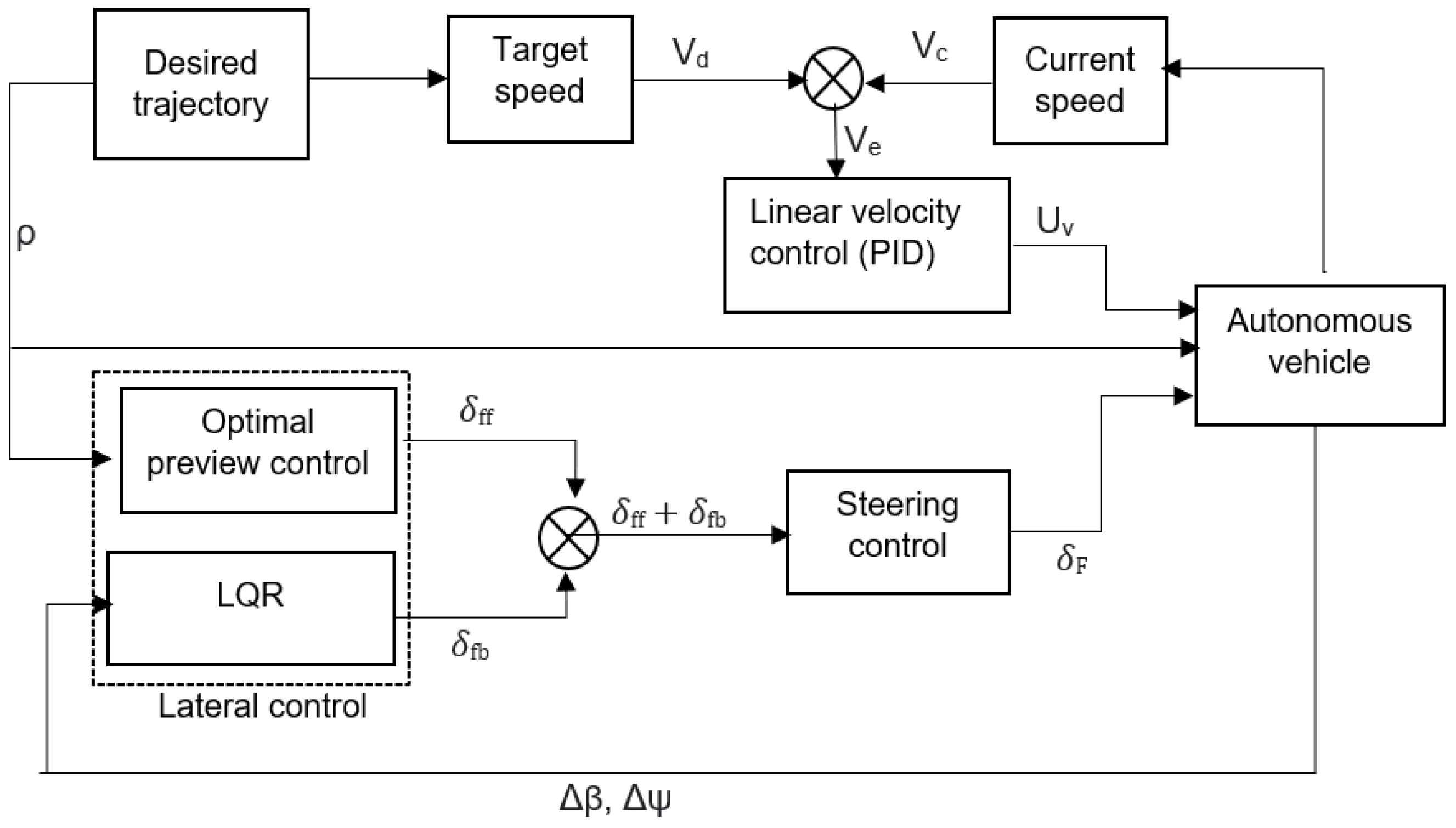
3.2. Lateral Controller
3.2.1. Optimal Preview Controller
3.2.2. Optimal LQR Controller
4. Experimental Results and Discussion
- Simulated path: There are 750 continuous points and five normal curves identified in the simulated path. Total distance of this trajectory is approximately 3.95 km, and the maximum speed limit is 20 km/h for the entire path.
- Real dataset: The total distance of the reference path (traveled path) is approximately 4.2 km, and the maximum speed is 20 km/h for the entire path. There are 1094 segment points determined after the preprocessing and analyzing of given GPS data. Fourteen sharp curves (dangerous curves) are detected in this trajectory with different geometric characteristics.
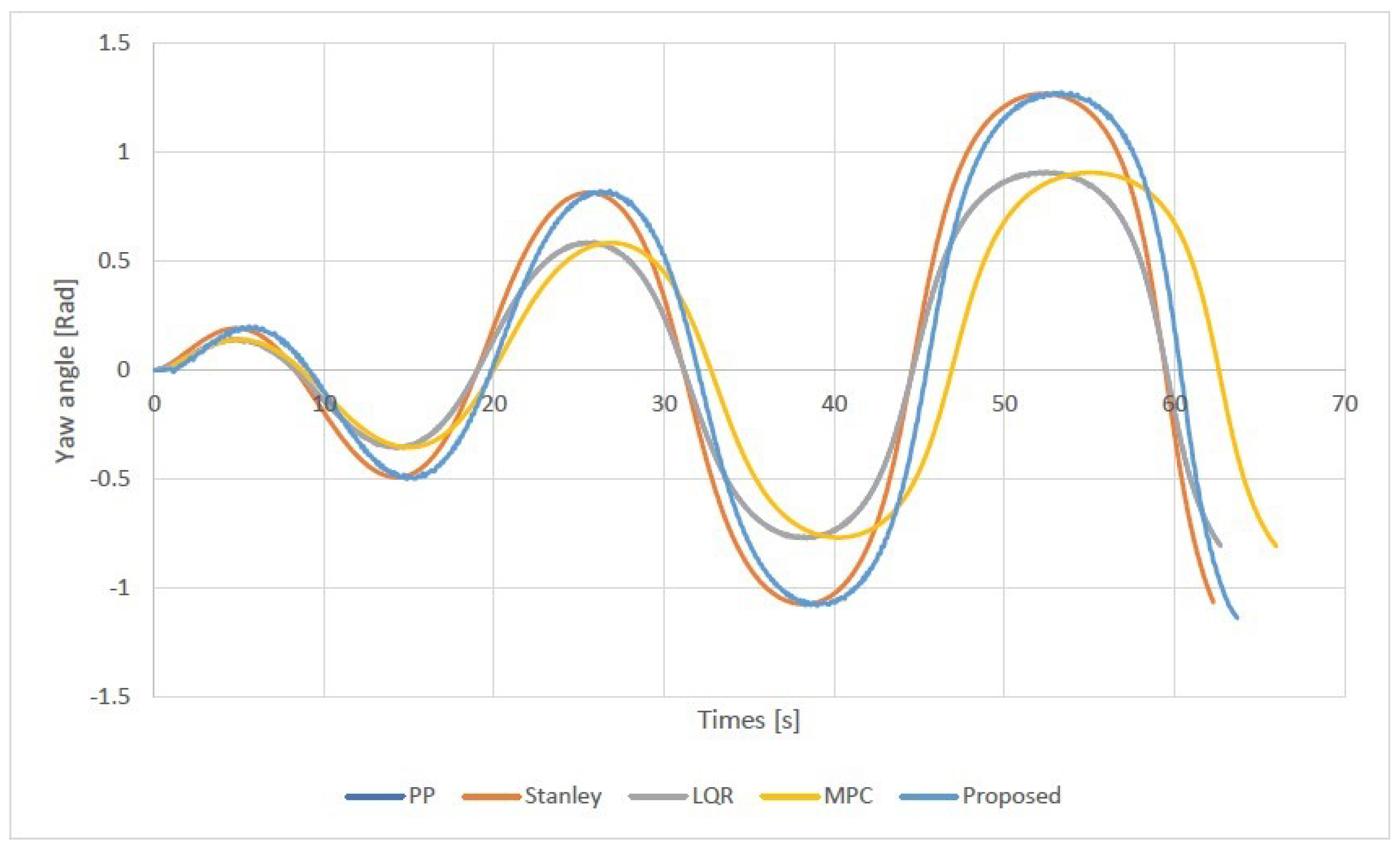
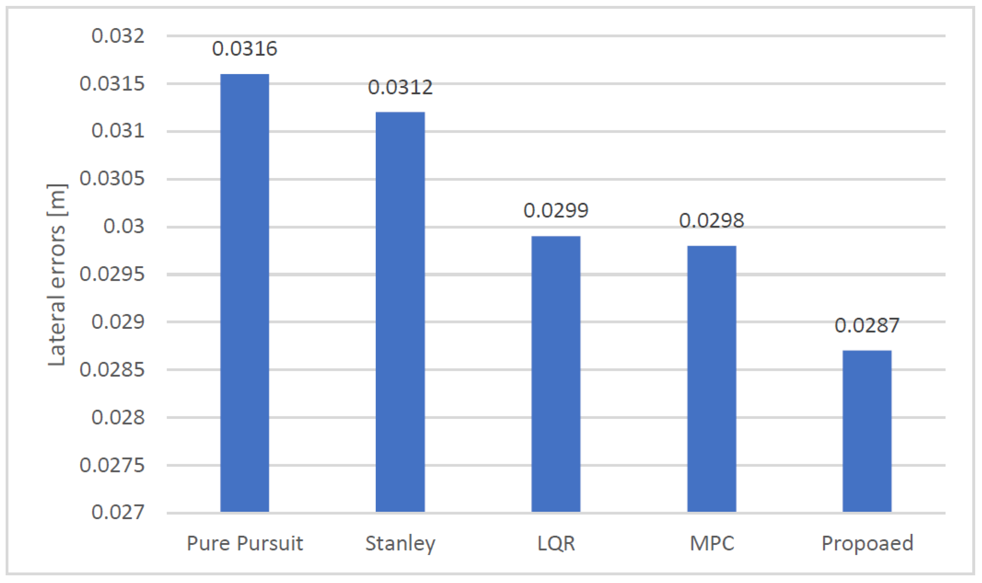
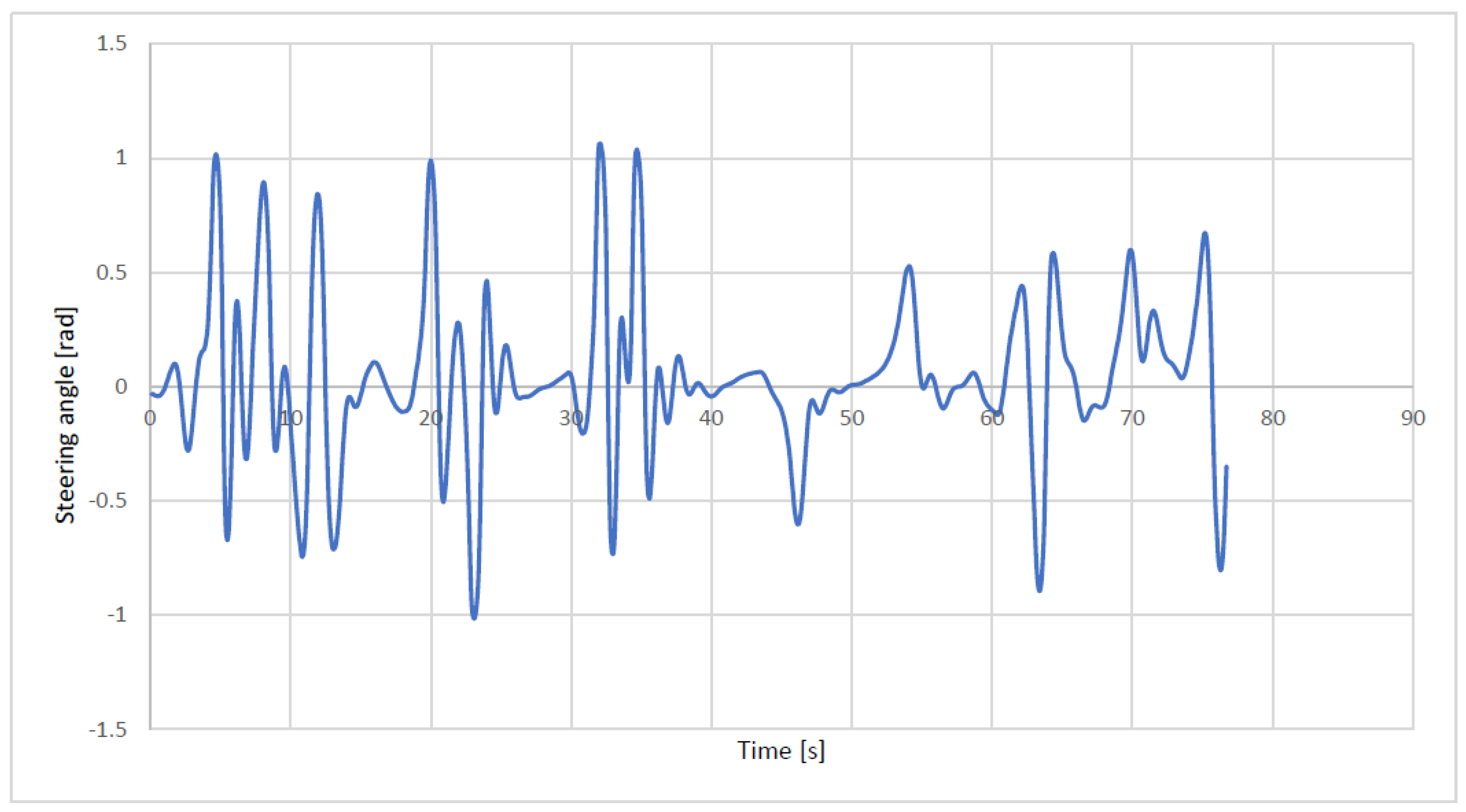
Experimental Results
5. Conclusions
Author Contributions
Funding
Institutional Review Board Statement
Informed Consent Statement
Data Availability Statement
Conflicts of Interest
References
- Cibooglu, M.; Karapinar, U.; Soylemez, M.T. Hybrid controller approach for an autonomous ground vehicle path tracking problem. In Proceedings of the 25th Mediterranean Conference on Control, Valletta, Malta, 3–6 July 2017; pp. 583–588. [Google Scholar] [CrossRef] [Green Version]
- Andersen, H.; Chong, Z.J.; Eng, Y.H.; Pendleton, S.; Ang, M.H. Geometric path tracking algorithm for autonomous driving in pedestrian environment. In Proceedings of the EEE International Conference on Advanced Intelligent Mechatronics (AIM), Banff, AB, Canada, 12–15 July 2016; pp. 1669–1674. [Google Scholar] [CrossRef]
- Coulter, R.C. Implementation of the Pure Pursuit Path Tracking Algorithm; Carnegie Mellon University: Pittsburgh, PA, USA, 1992. [Google Scholar]
- Corke, P. Robotics, Vision and Control—Fundamental Algorithms in MATLAB; Springer: Cham, Switzerland, 2011. [Google Scholar] [CrossRef] [Green Version]
- Wit, J.C., III; Carl, D.; Armstrong, D. Autonomous ground vehicle path tracking. J. Robot. Syst. 2004, 21, 439–449. [Google Scholar] [CrossRef]
- Park, M.-W.; Lee, S.-W.; Han, W.-Y. Development of lateral control system for autonomous vehicle based on adaptive pure pursuit algorithm. In Proceedings of the 14th International Conference on Control, Automation and Systems (ICCAS 2014), Gyeonggi-do, Korea, 22–25 October 2014; pp. 1443–1447. [Google Scholar] [CrossRef]
- Wang, W.-J.; Hsu, T.-M.; Wu, T.-S. The improved pure pursuit algorithm for autonomous driving advanced system. In Proceedings of the IEEE 10th International Workshop on Computational Intelligence and Applications (IWCIA), Hiroshima, Japan, 11–12 November 2017; pp. 33–38. [Google Scholar] [CrossRef]
- Amer, N.H.; Zamzuri, H.; Hudha, K.; Aparow, V.R.; Kadir, Z.A.; Abidin, A.F.Z. Path tracking controller of an autonomous armoured vehicle using modified Stanley controller optimized with particle swarm optimization. J. Braz. Soc. Mech. Sci. Eng. 2018, 40, 104. [Google Scholar] [CrossRef]
- Hoffman, G.M.; Tomlin, C.J.; Montemerlo, M.; Thrun, S. Autonomous Automobile Trajectory Tracking for Off-Road Drriv-ing: Controller Design, Experimental Validation and Racing. In Proceedings of the American Control Conference, New York, NY, USA, 9–13 July 2007; pp. 2296–2301. [Google Scholar] [CrossRef]
- Yang, J.; Bao, H.; Ma, N.; Xuan, Z. An Algorithm of Curved Path Tracking with Prediction Model for Autonomous Vehicle. In Proceedings of the 13th International Conference on Computational Intelligence and Security (CIS), Hong Kong, China, 15–18 December 2017; pp. 405–408. [Google Scholar] [CrossRef]
- Dul, F.; Lichota, P.; Rusowicz, A. Generalized Linear Quadratic Control for a Full Tracking Problem in Aviation. J. Sens. 2020, 20, 2955. [Google Scholar] [CrossRef] [PubMed]
- Salehpour, S.; Pourasad, Y.; Taheri, S. Vehicle path tracking by integrated chassis control. J. Cent. South Univ. 2015, 22, 1378–1388. [Google Scholar] [CrossRef]
- Birla, N.; Swarup, A. Optimal preview control: A review. J. Optim. Control Appl. Methods 2015, 36, 241–268. [Google Scholar] [CrossRef]
- Tomizuka, M. Optimal continuous finite preview problem. IEEE Trans. Autom. Control 1975, 20, 362–365. [Google Scholar] [CrossRef]
- Sheridan, T. Three Models of Preview Control. IEEE Trans. Hum. Factors Electron. 1966, HFE-7, 91–102. [Google Scholar] [CrossRef]
- Hać, A. Optimal Linear Preview Control of Active Vehicle Suspension. Veh. Syst. Dyn. 1992, 21, 167–195. [Google Scholar] [CrossRef]
- Hayase, M.; Ichikawa, K. Optimal Servosystem Utilizing Future Value of Desired Function. Trans. Soc. Instrum. Control Eng. 1969, 5, 86–94. [Google Scholar] [CrossRef] [Green Version]
- Katayama, T.; Ohki, T.; Inoue, T.; Kato, T. Design of an optimal controller for a discrete-time system subject to previewable demand. Int. J. Control 1985, 41, 677–699. [Google Scholar] [CrossRef]
- Liao, F.; Tang, Y.Y.; Liu, H.; Wang, Y. Design of an Optimal Preview Controller for Continuous-Time Systems. Int. J. Wave-Lets Multiresolut. Inf. Process 2011, 9, 655–673. [Google Scholar] [CrossRef]
- Zhang, W.; Bae, J.; Tomizuka, M. Modified Preview Control for a Wireless Tracking Control System with Packet Loss. IEEE/ASME Trans. Mechatronics 2015, 20, 299–307. [Google Scholar] [CrossRef]
- Wu, J.; Liao, F.; Tomizuka, M. Optimal preview control for a linear continuous-time stochastic control system in finite-time horizon. Int. J. Syst. Sci. 2016, 48, 129–137. [Google Scholar] [CrossRef]
- Zhen, Z.-Y.; Wang, Z.-S.; Wang, D.-B. Information Fusion Estimation Based Preview Control for Discrete Linear System. Acta Autom. Sin. 2010, 36, 347–352. [Google Scholar] [CrossRef]
- Zhen, Z.-Y.; Wang, Z.-S.; Wang, D.-B. Optimal preview tracking control based on information fusion in error system. Kongzhi Lilun Yu Yingyong/Control Theory Appl. 2009, 26, 425–428. [Google Scholar]
- Cao, M.; Liao, F. Design of an optimal preview controller for linear discrete-time descriptor systems with state delay. Int. J. Syst. Sci. 2015, 46, 932–943. [Google Scholar] [CrossRef]
- Lu, Y.; Liao, F.; Deng, J.; Pattinson, C. Cooperative optimal preview tracking for linear descriptor multi-agent systems. J. Frankl. Inst. 2018, 356, 908–934. [Google Scholar] [CrossRef] [Green Version]
- Li, Z.; Chitturi, M.V.; Bill, A.R.; Noyce, D.A. Automated Identification and Extraction of Horizontal Curve Information from Geographic Information System Roadway Maps. Transp. Res. Rec. J. Transp. Res. Board 2012, 2291, 80–92. [Google Scholar] [CrossRef] [Green Version]
- Årzén, K.-E.; Johansson, M.; Babuška, R. Fuzzy Control Versus Conventional Control. In Fuzzy Algorithms for Control; Verbruggen, H.B., Zimmermann, H.-J., Babuška, R., Eds.; Springer: Dordrecht, The Netherlands, 1999; pp. 59–81. [Google Scholar]
- Baturone, I.; Moreno-Velo, F.; Sanchez-Solano, S.; Ollero, A. Automatic Design of Fuzzy Controllers for Car-Like Autonomous Robots. IEEE Trans. Fuzzy Syst. 2004, 12, 447–465. [Google Scholar] [CrossRef] [Green Version]
- Li, T.-H.S; Chang, S.-J. Autonomous fuzzy parking control of a car-like mobile robot. IEEE Trans. Syst. Man Cybern. Part A Syst. Hum. 2003, 33, 451–465. [Google Scholar] [CrossRef]
- Lee, T.; Lam, H.; Leung, F.; Tam, P. A practical fuzzy logic controller for the path tracking of wheeled mobile robots. IEEE Control Syst. 2003, 23, 60–65. [Google Scholar] [CrossRef]
- Sanchez, O.F.A.; Ollero, A.; Heredia, G. Adaptive fuzzy control for automatic path tracking of outdoor mobile robots. Application to Romeo 3R. In Proceedings of the 6th International Fuzzy Systems Conference, Barcelona, Spain, 5 July 1997; Volume 1, pp. 593–599. [Google Scholar] [CrossRef]
- Vans, E.; Vachkov, G.; Sharma, A. Vision based autonomous path tracking of a mobile robot using fuzzy logic. In Proceedings of the Asia-Pacific World Congress on Computer Science and Engineering, Nadi, Fiji, 4–5 November 2014; pp. 1–8. [Google Scholar] [CrossRef]
- Guo, J.; Hu, P.; Li, L.; Wang, R. Design of Automatic Steering Controller for Trajectory Tracking of Unmanned Vehicles Using Genetic Algorithms. IEEE Trans. Veh. Technol. 2012, 61, 2913–2924. [Google Scholar] [CrossRef]
- Luo, C. Neural-network-based fuzzy logic tracking control of mobile robots. In Proceedings of the 13th IEEE Conference on Automation Science and Engineering (CASE), Xi’an, China, 20–23 August 2017; pp. 1318–1319. [Google Scholar] [CrossRef]
- Kayacan, E.; Ramon, H.; Saeys, W. Robust Trajectory Tracking Error Model-Based Predictive Control for Unmanned Ground Vehicles. IEEE/ASME Trans. Mechatron. 2016, 21, 806–814. [Google Scholar] [CrossRef]
- Guo, H.; Liu, J.; Cao, D.; Chen, H.; Yu, R.; Lv, C. Du-al-envelop-oriented moving horizon path tracking control for fully automated vehicles. Mechatronics 2018, 50, 422–433. [Google Scholar] [CrossRef] [Green Version]
- Mayne, D.Q. Model predictive control: Recent developments and future promise. Automatica 2004, 50, 2967–2986. [Google Scholar] [CrossRef]
- Li, S.; Wang, G.; Guo, L.; Zheng, L.; Li, X.; Yu, Z.; Cui, G.; Zhang, J. NMPC-Based Yaw Stability Control by Active Front Wheel Steering. IFAC PapersOnLine 2018, 51, 583–588. [Google Scholar] [CrossRef]
- Yu, H.; Duan, J.; Taheri, S.; Cheng, H.; Qi, Z. A model predictive control approach combined unscented Kalman filter vehicle state estimation in intelligent vehicle trajectory tracking. Adv. Mech. Eng. 2015, 7, 1687814015578361. [Google Scholar] [CrossRef] [Green Version]
- Falcone, P.; Borrelli, F.; Asgari, J.; Tseng, H.E.; Hrovat, D. Predictive active steering control for autonomous vehicle systems. IEEE Trans. Control Syst. Technol. 2007, 15, 566–580. [Google Scholar] [CrossRef]
- Zhang, L.; Wu, G. Combination of Front Steering and Differential Braking Control for the Path Tracking of Autonomous Vehicle; SAE Technical Paper; SAE International: Warrendale, PA, USA, 2016. [Google Scholar] [CrossRef]
- Yao, Z.; Jiang, H.; Cheng, Y.; Jiang, Y.; Ran, B. Integrated Schedule and Trajectory Optimization for Connected Automated Vehicles in a Conflict Zone. IEEE Trans. Intell. Transp. Syst. 2020, 23, 1841–1851. [Google Scholar] [CrossRef]
- Brumercik, F.; Lukac, M.; Caban, J. Unconventional Powertrain Simulatiion. Commun. Sci. Lett. Univ. Zilina 2016, 18, 30–33. [Google Scholar] [CrossRef]
- De-Las-Heras, G.; Sánchez-Soriano, J.; Puertas, E. Advanced Driver Assistance Systems (ADAS) Based on Machine Learning Techniques for the Detection and Transcription of Variable Message Signs on Roads. Sensors 2021, 21, 5866. [Google Scholar] [CrossRef] [PubMed]
- Nie, X.; Min, C.; Pan, Y.; Li, K.; Li, Z. Deep-Neural Network-Based Modelling of Longitudinal-Lateral Dynamics to Predict the Vehicle States for Autonomous Driving. Sensors 2022, 22, 2013. [Google Scholar] [CrossRef] [PubMed]
- Gámez Serna, C.; Ruichek, Y. Dynamic Speed Adaptation for Path Tracking Based on Curvature Information and Speed Limits. Sensors 2017, 17, 1383. [Google Scholar] [CrossRef] [PubMed] [Green Version]
- Snider, J. Automatic Steering Methods for Autonomous Automobile Path Tracking; Number CMU-RI-TR-09-08; Institution Carnegie Mellon University: Pittsburgh, PA, USA, 2009. [Google Scholar]
- Macadam, C.C. Application of an Optimal Preview Control for Simulation of Closed-Loop Automobile Driving. IEEE Trans. Syst. Man, Cybern. 1981, 11, 393–399. [Google Scholar] [CrossRef]
- Farooq, A.; Limebeer, D. Path following of Optimal Trajectories Using Preview Control. In Proceedings of the 44th IEEE Conference on Decision and Control, Seville, Spain, 15 December 2005; pp. 2787–2792. [Google Scholar] [CrossRef]


| Parameter | Value | Description |
|---|---|---|
| M | 1155.0 kg | Vehicle mass |
| W | 1.6 m | Width of vehicle |
| I | 1466.35 kgm | Vehicle yaw moment inertia |
| WB | 2.6 m | Wheel base |
| TR | 0.33 m | Tyre radius |
| TW | 0.21 m | Tyre width |
| 1.165 m | Distances of front tire from the C.G of the vehicle | |
| 1.165 m | Distances of rear tire from the C.G of the vehicle | |
| 162,835.82 N/rad | Cornering stiffness of front tyre | |
| 162,835.82 N/rad | Cornering stiffness of rear tyre |
| Curve | PP | Stanley | LQR | MPC | Proposed |
|---|---|---|---|---|---|
| 1 | 0.0201 | 0.0192 | 0.0163 | 0.0182 | 0.0156 |
| 2 | 0.0238 | 0.0231 | 0.0199 | 0.0193 | 0.0185 |
| 3 | 0.0310 | 0.0309 | 0.0306 | 0.0301 | 0.0291 |
| 4 | 0.0431 | 0.0428 | 0.0421 | 0.0415 | 0.0404 |
| 5 | 0.0404 | 0.0403 | 0.0403 | 0.0403 | 0.0396 |
| Average | 0.0316 | 0.0312 | 0.0299 | 0.0298 | 0.0287 |
| Travel time | 63 s | 63 s | 63 s | 63 s | 63 s |
| Curve | PP | Stanley | LQR | MPC | Proposed |
|---|---|---|---|---|---|
| 1 | 0.1915 | 0.1403 | 0.1384 | 0.0504 | 0.0905 |
| 2 | 0.2341 | 0.1619 | 0.1398 | 0.0992 | 0.0910 |
| 3 | 0.2096 | 0.1534 | 0.1275 | 0.0549 | 0.0531 |
| 4 | 0.1101 | 0.1041 | 0.1007 | 0.0481 | 0.0467 |
| 5 | 0.1305 | 0.1253 | 0.1131 | 0.0918 | 0.0685 |
| 6 | 0.5039 | 0.3580 | 0.3169 | 0.2727 | 0.1553 |
| 7 | 0.6321 | 0.3337 | 0.2744 | 0.2809 | 0.1561 |
| 8 | 0.6909 | 0.3824 | 0.3410 | 0.2901 | 0.1624 |
| 9 | 0.6911 | 0.3773 | 0.3305 | 0.2903 | 0.1631 |
| 10 | 0.0873 | 0.0851 | 0.0822 | 0.0814 | 0.0752 |
| 11 | 0.0817 | 0.0803 | 0.0813 | 0.0883 | 0.0747 |
| 12 | 0.1544 | 0.1032 | 0.0949 | 0.0621 | 0.0533 |
| 13 | 0.0909 | 0.0906 | 0.0871 | 0.0710 | 0.0651 |
| 14 | 0.1192 | 0.1126 | 0.1008 | 0.1098 | 0.0801 |
| Average | 0.2805 | 0.1863 | 0.1663 | 0.1350 | 0.0953 |
| Travel time | 78 s | 79 s | 79 s | 78 s | 82 s |
Publisher’s Note: MDPI stays neutral with regard to jurisdictional claims in published maps and institutional affiliations. |
© 2022 by the authors. Licensee MDPI, Basel, Switzerland. This article is an open access article distributed under the terms and conditions of the Creative Commons Attribution (CC BY) license (https://creativecommons.org/licenses/by/4.0/).
Share and Cite
Hossain, T.; Habibullah, H.; Islam, R. Steering and Speed Control System Design for Autonomous Vehicles by Developing an Optimal Hybrid Controller to Track Reference Trajectory. Machines 2022, 10, 420. https://doi.org/10.3390/machines10060420
Hossain T, Habibullah H, Islam R. Steering and Speed Control System Design for Autonomous Vehicles by Developing an Optimal Hybrid Controller to Track Reference Trajectory. Machines. 2022; 10(6):420. https://doi.org/10.3390/machines10060420
Chicago/Turabian StyleHossain, Tagor, Habib Habibullah, and Rafiqul Islam. 2022. "Steering and Speed Control System Design for Autonomous Vehicles by Developing an Optimal Hybrid Controller to Track Reference Trajectory" Machines 10, no. 6: 420. https://doi.org/10.3390/machines10060420