
Numerical Simulation and Analysis of the Flow Characteristics of the Roof-Attached Vortex (RAV) in a Closed Pump Sump


Abstract
:1. Introduction
2. Research Model and Numerical Calculation
2.1. Governing Equation
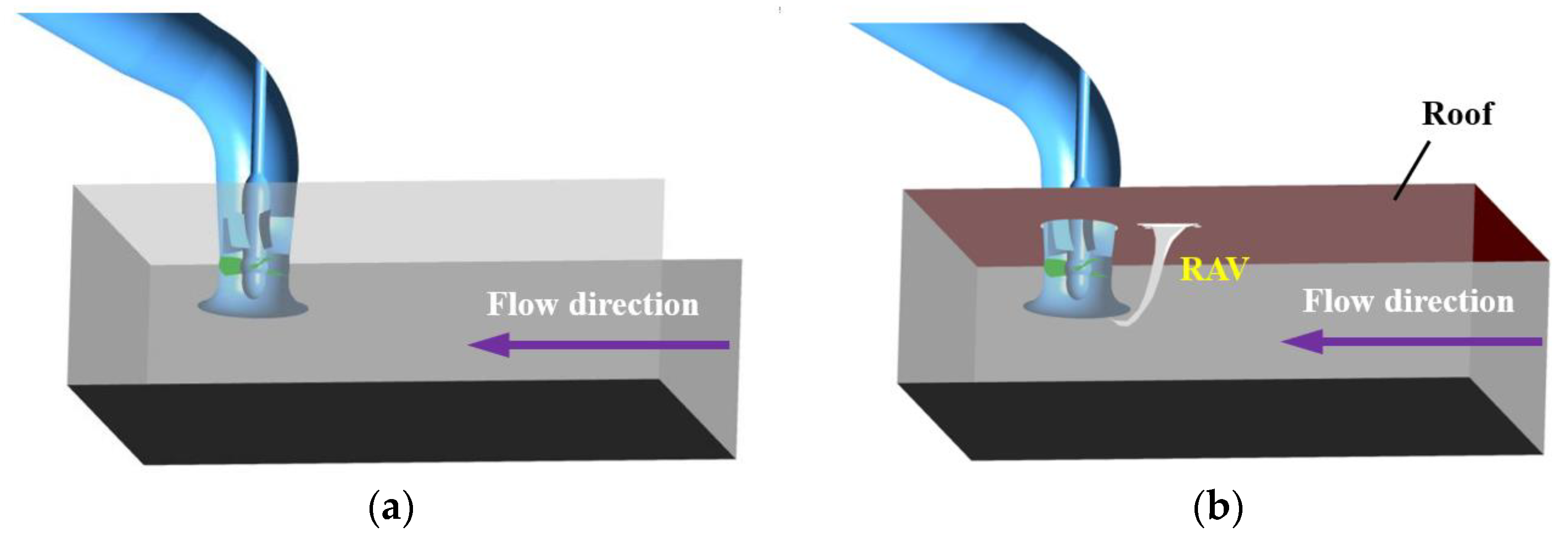
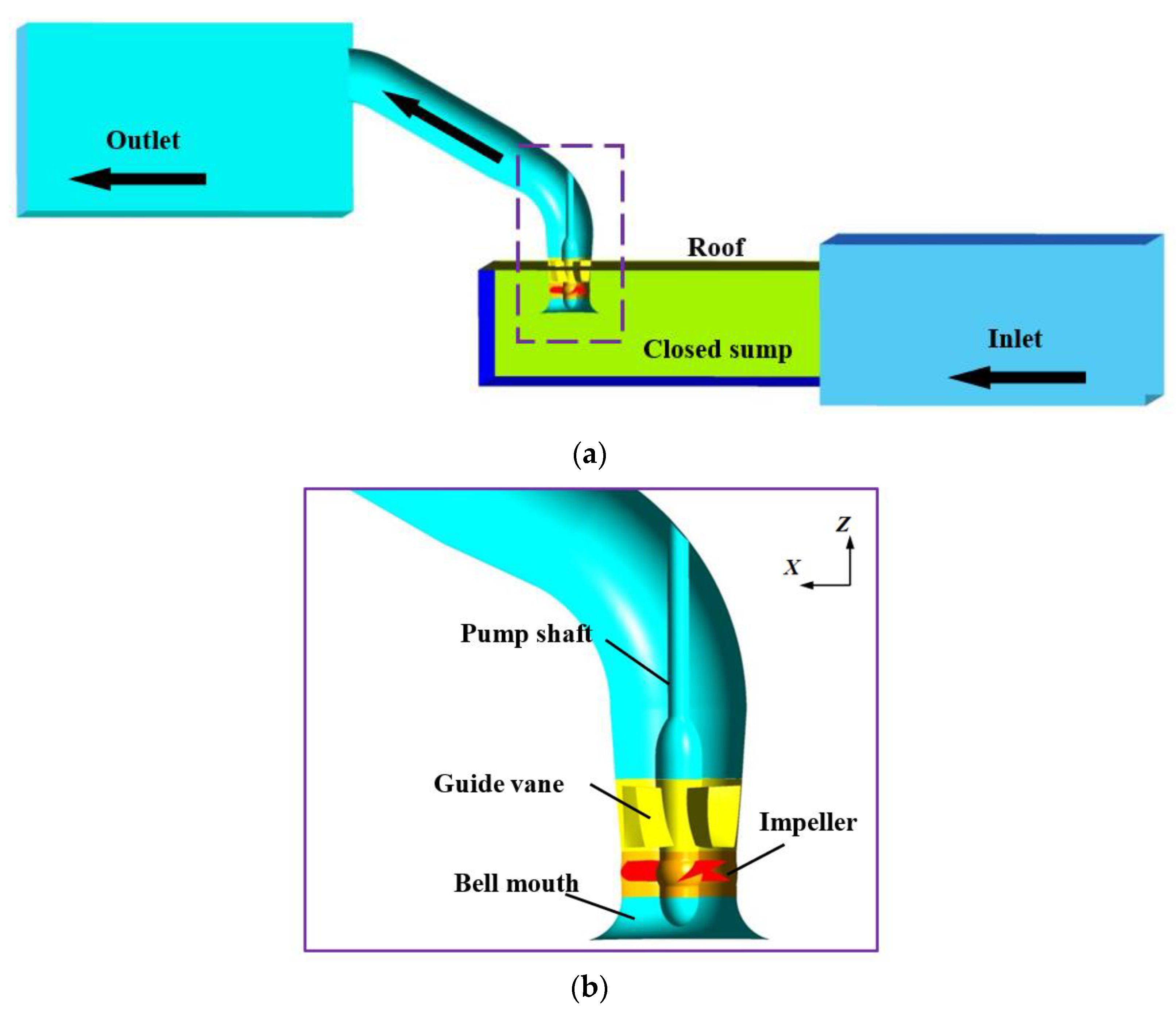
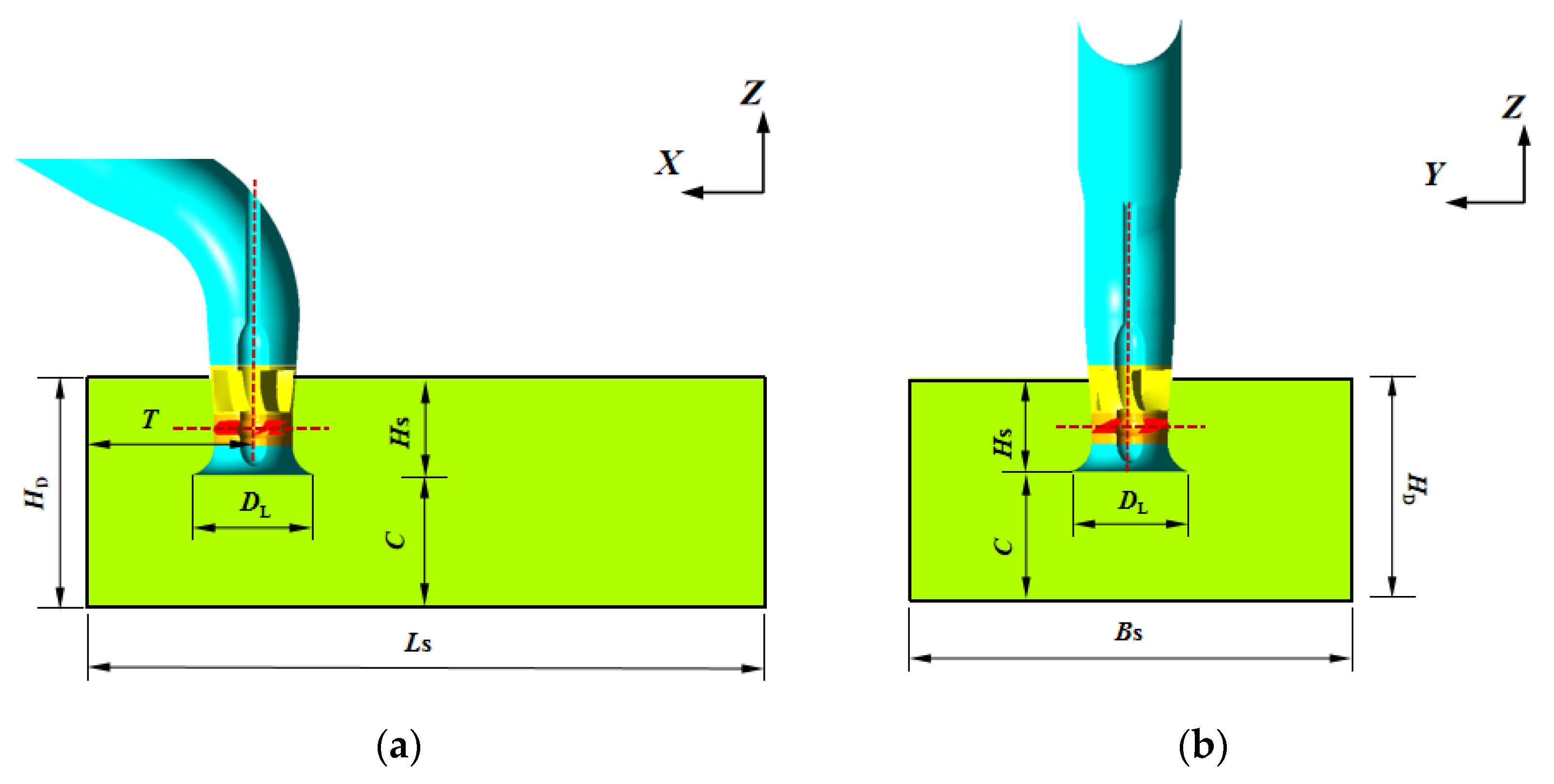
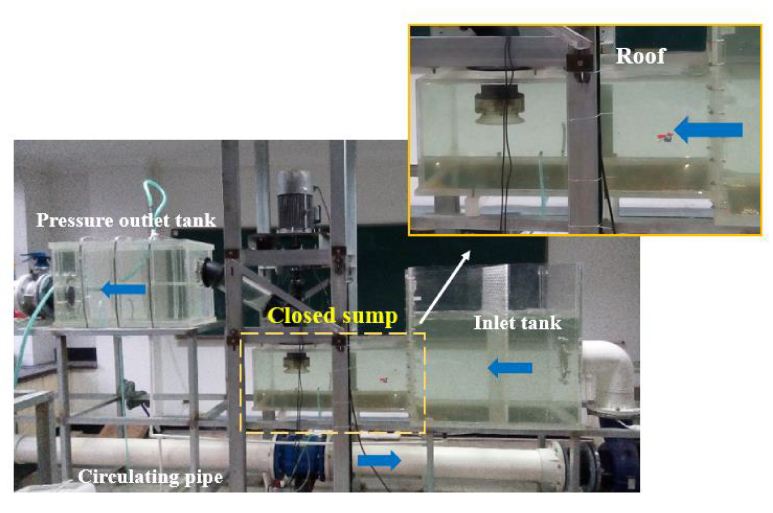
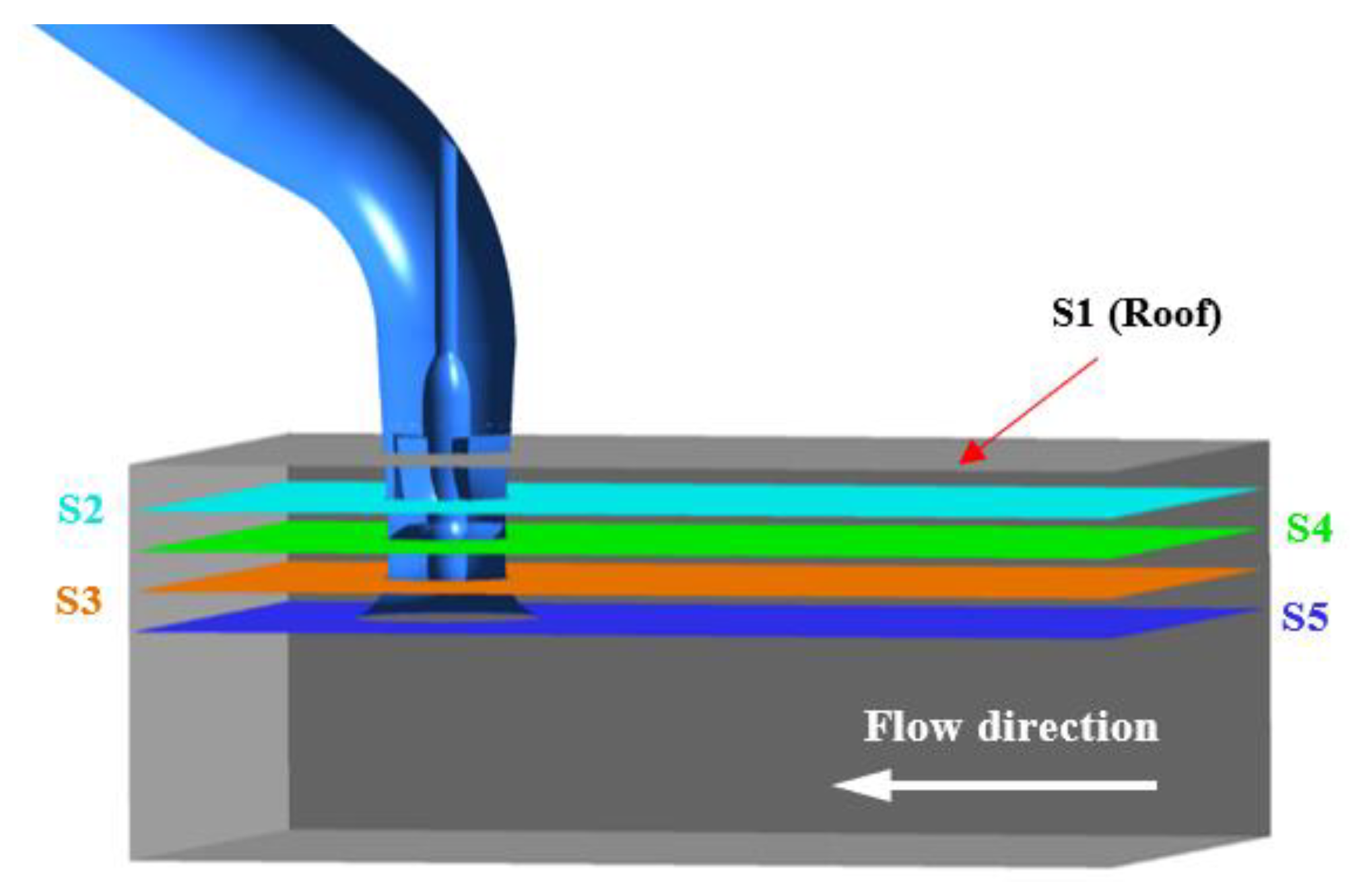
2.2. Research Model
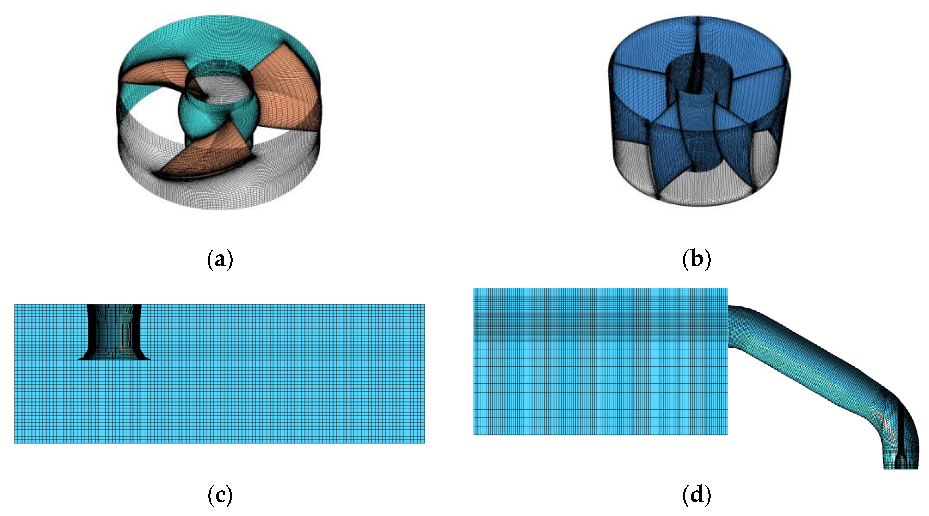
2.3. Grid Study
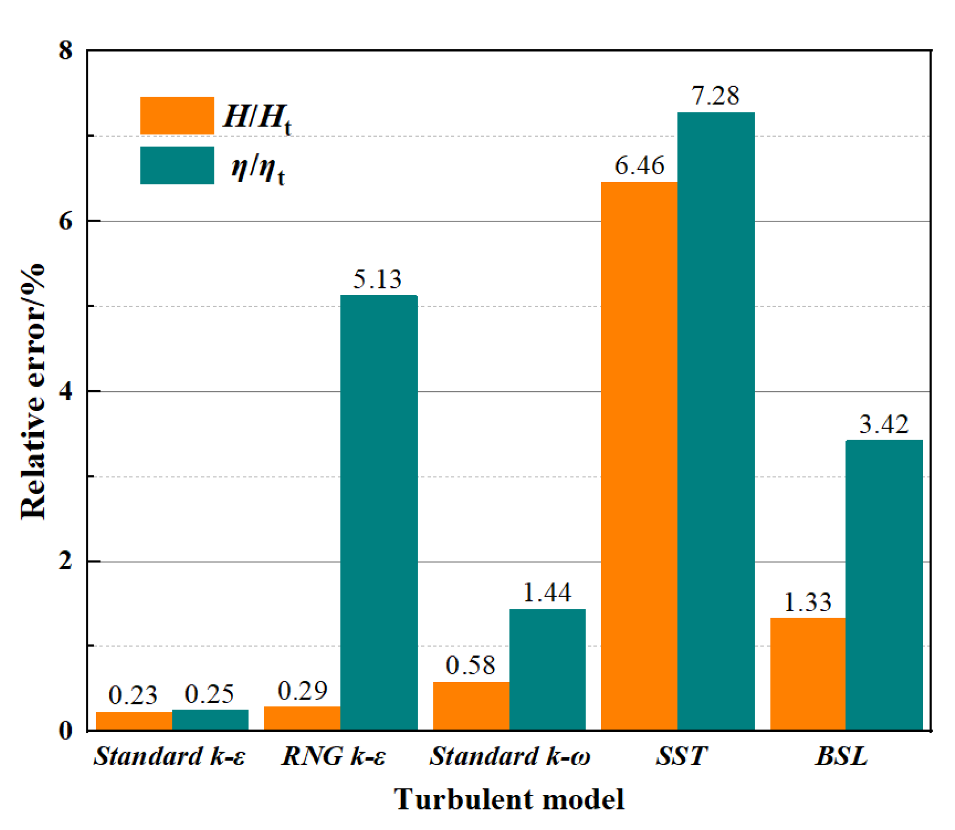
2.4. Turbulence Model
2.5. Calculation Parameter Settings
3. Results
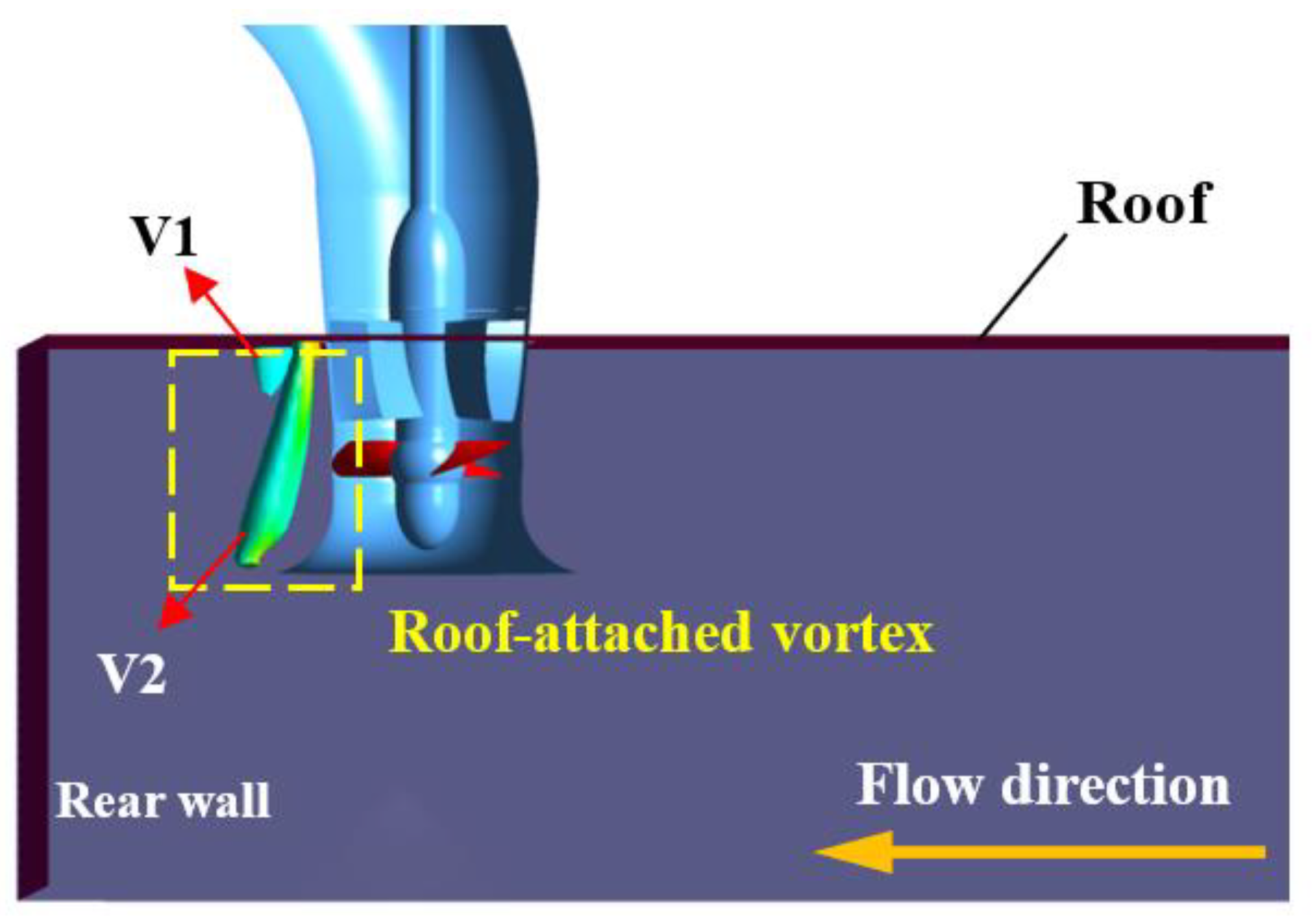
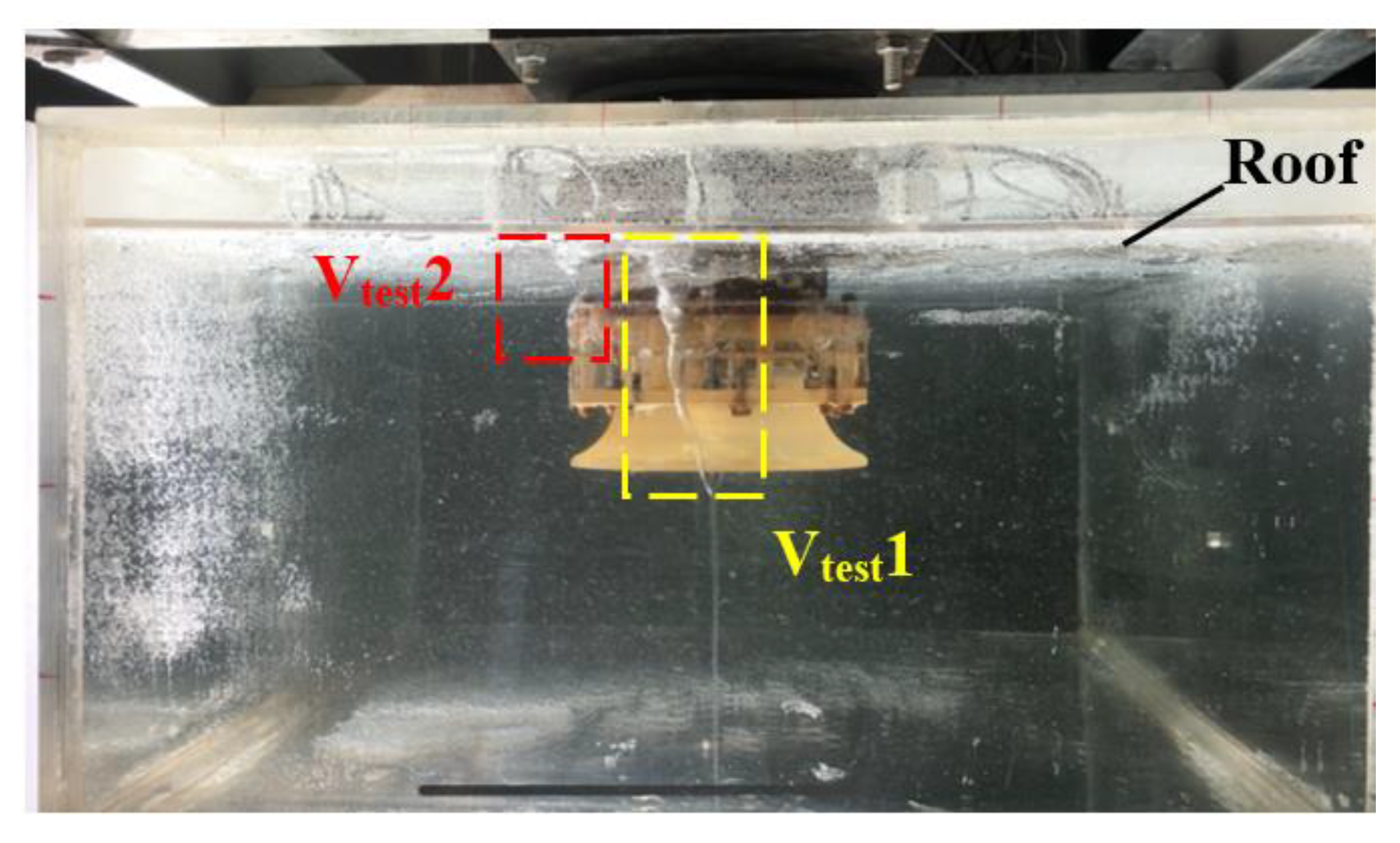
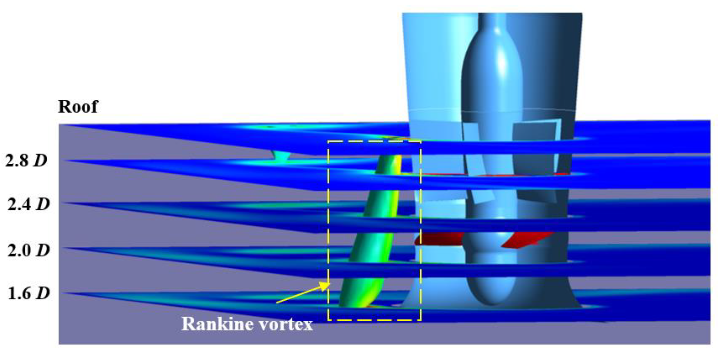
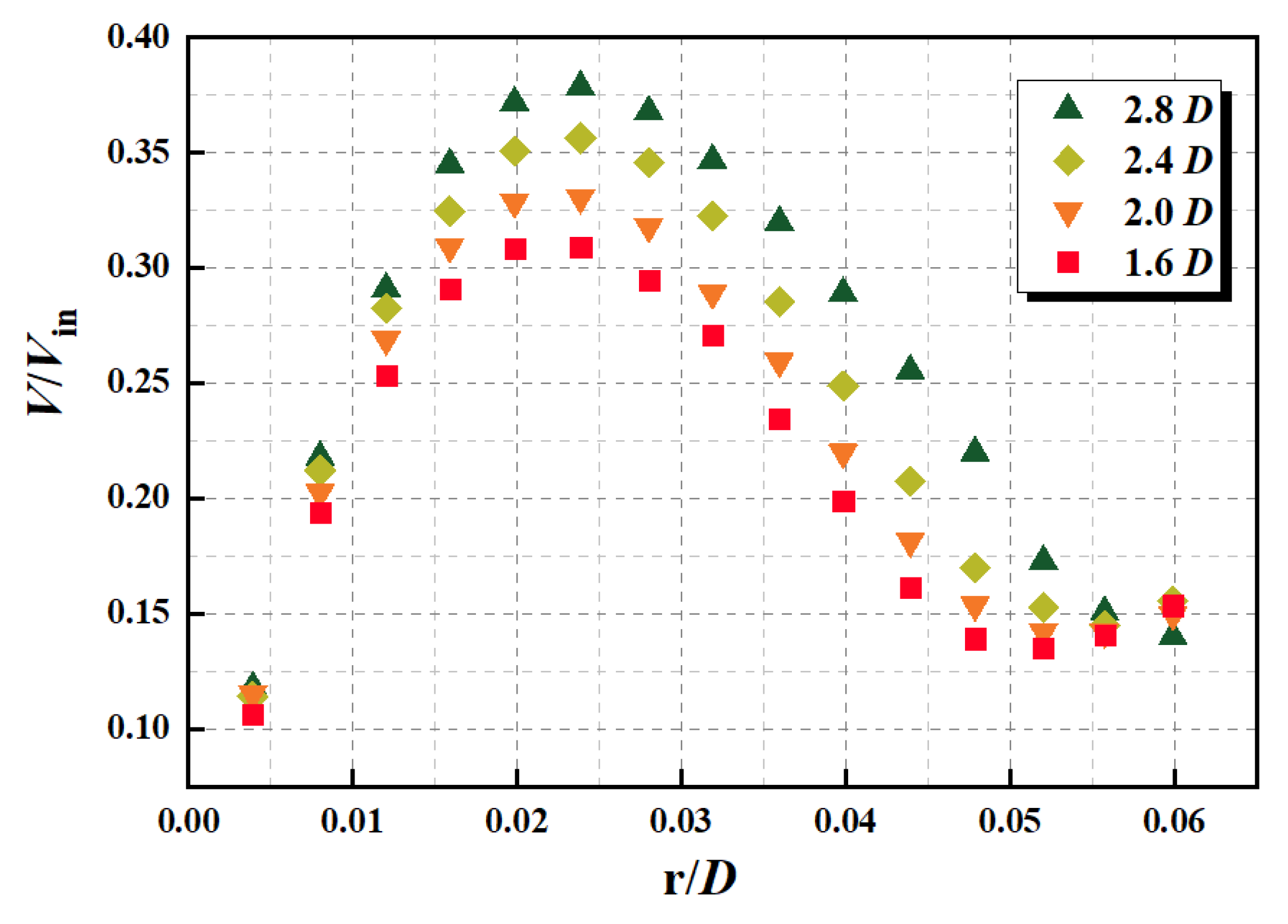
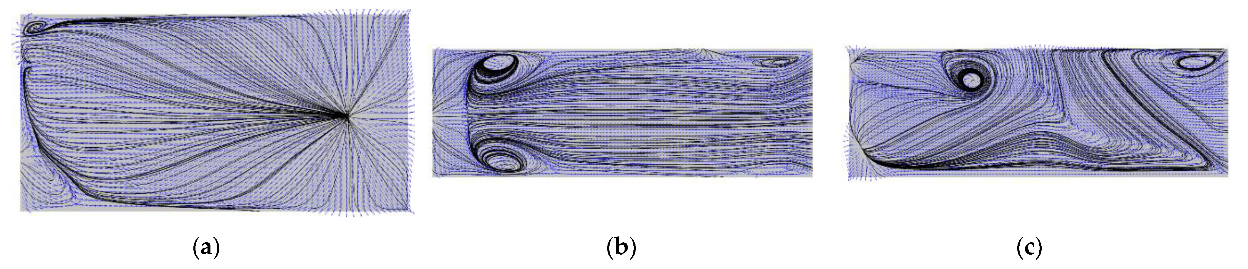
3.1. Distribution Characteristics of RAV
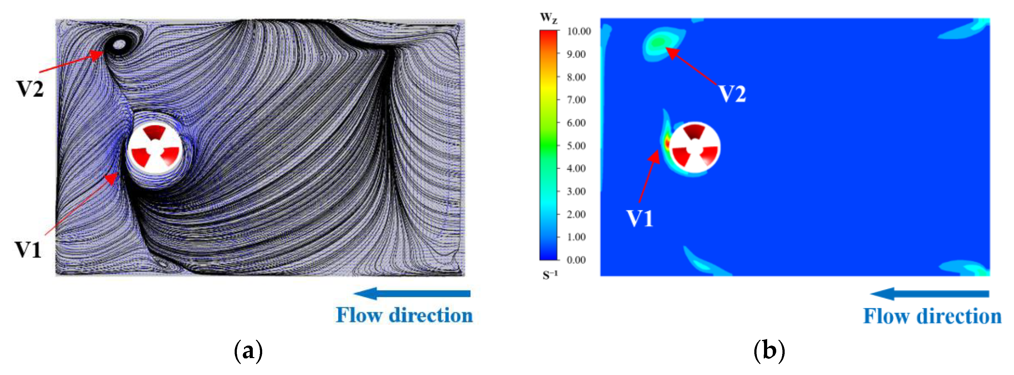
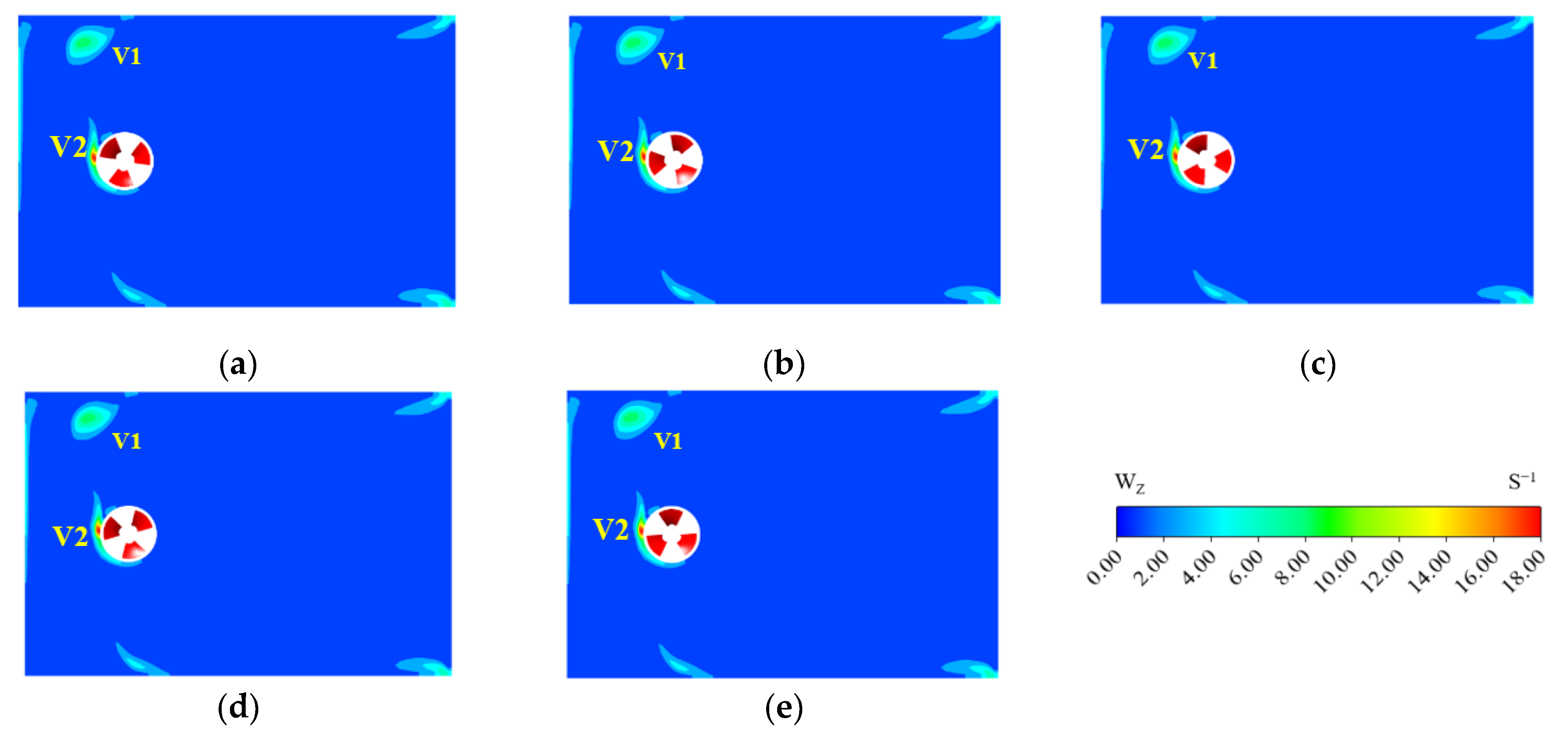
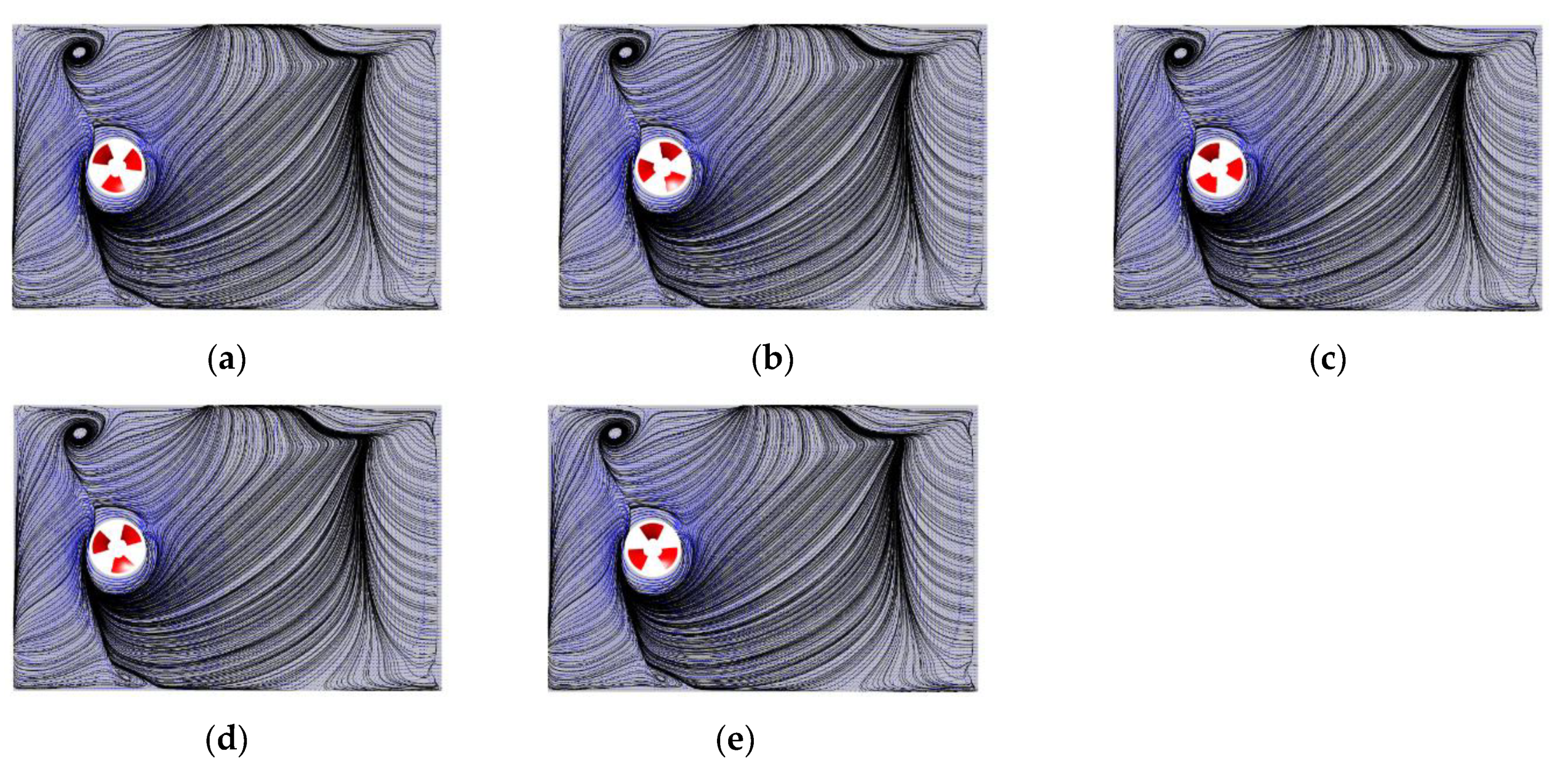
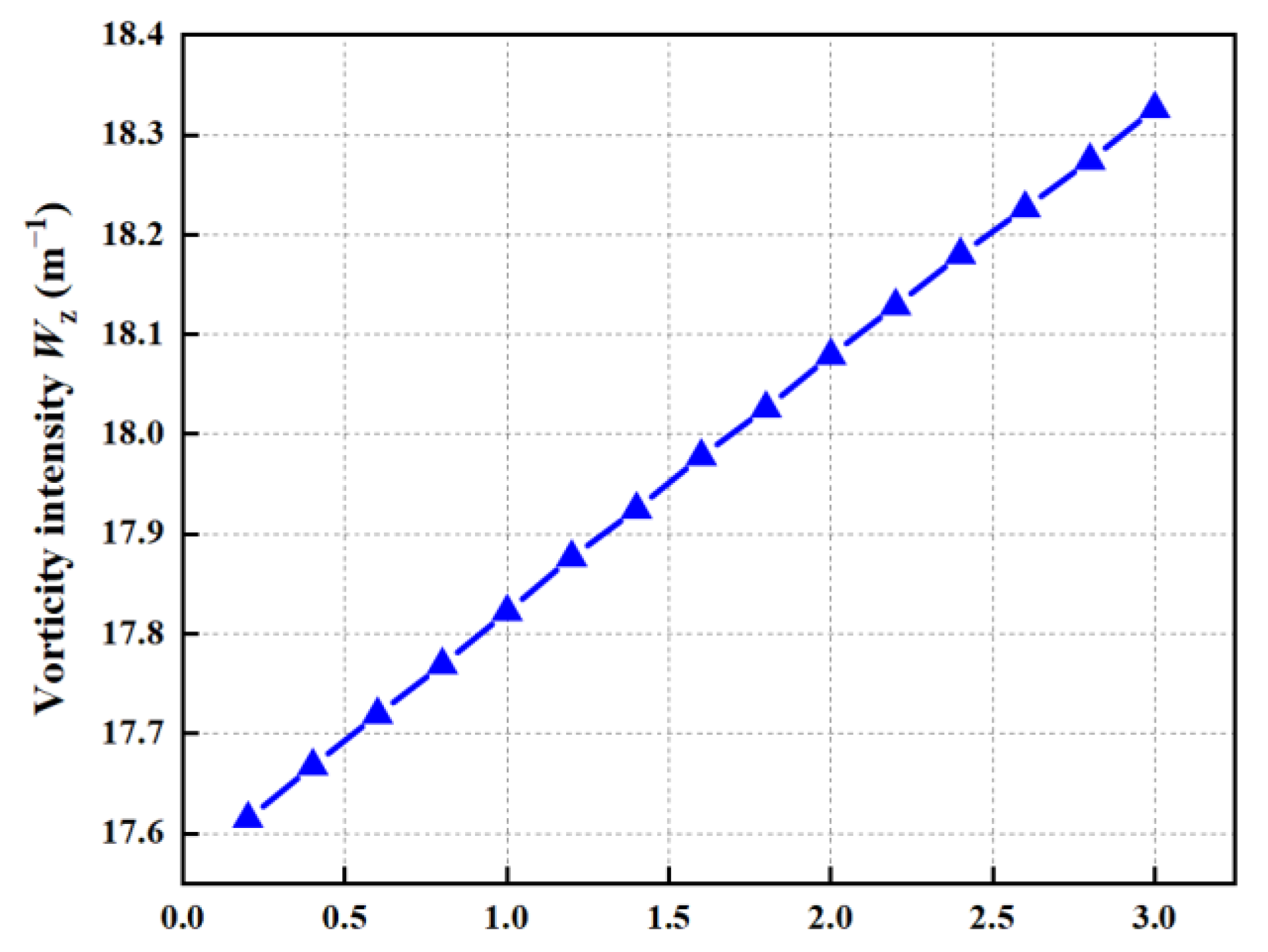
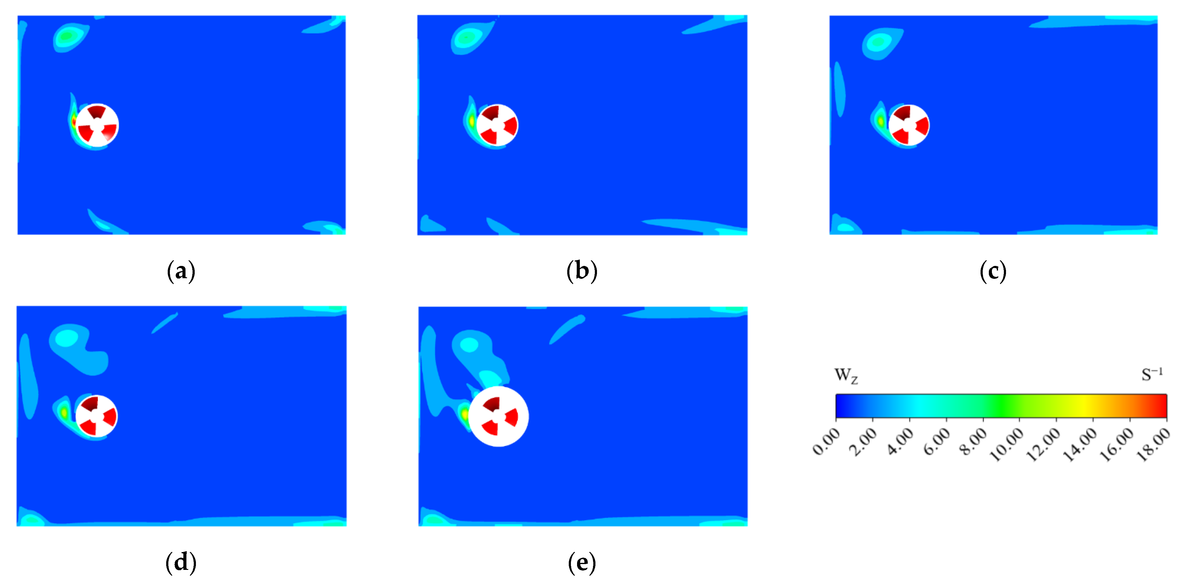
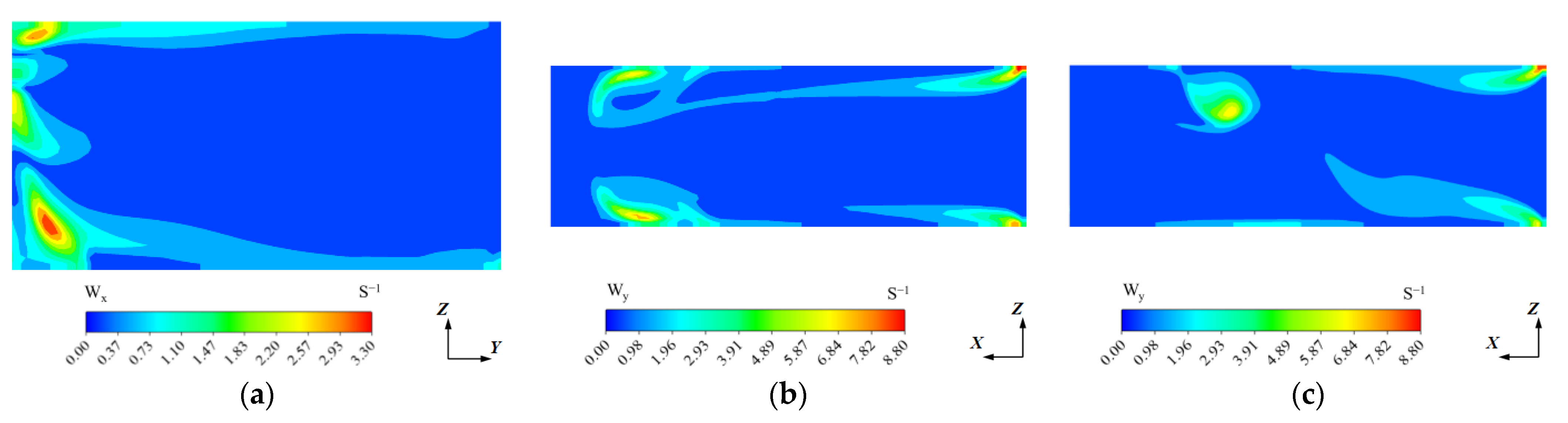
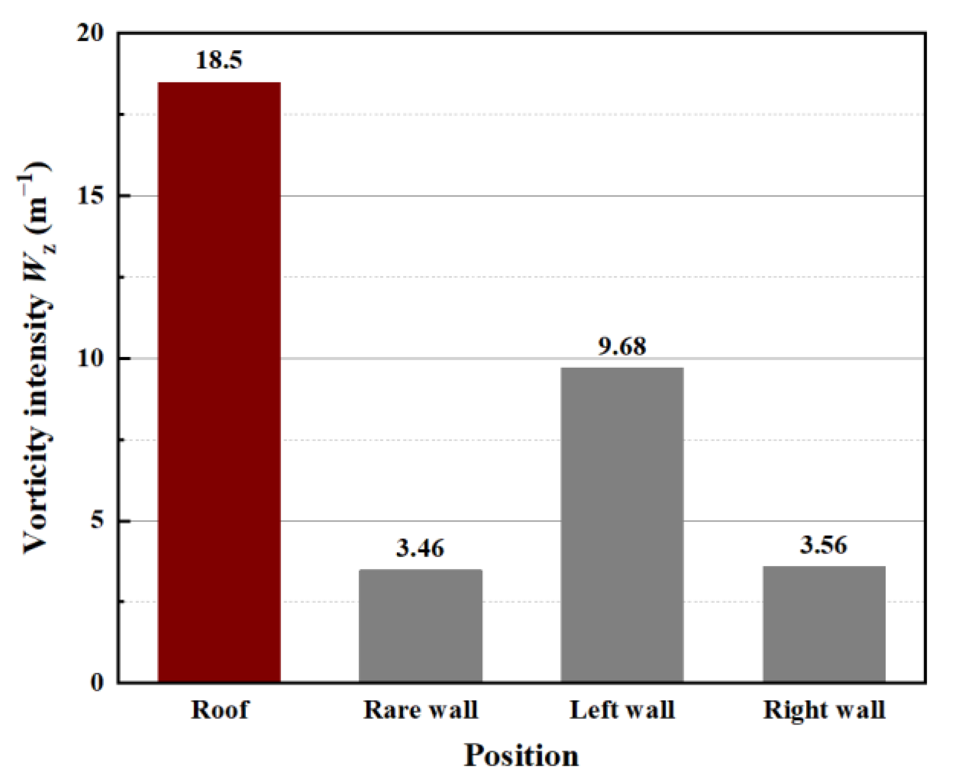
3.2. Distribution Characteristics of the Wall Vorticity Field
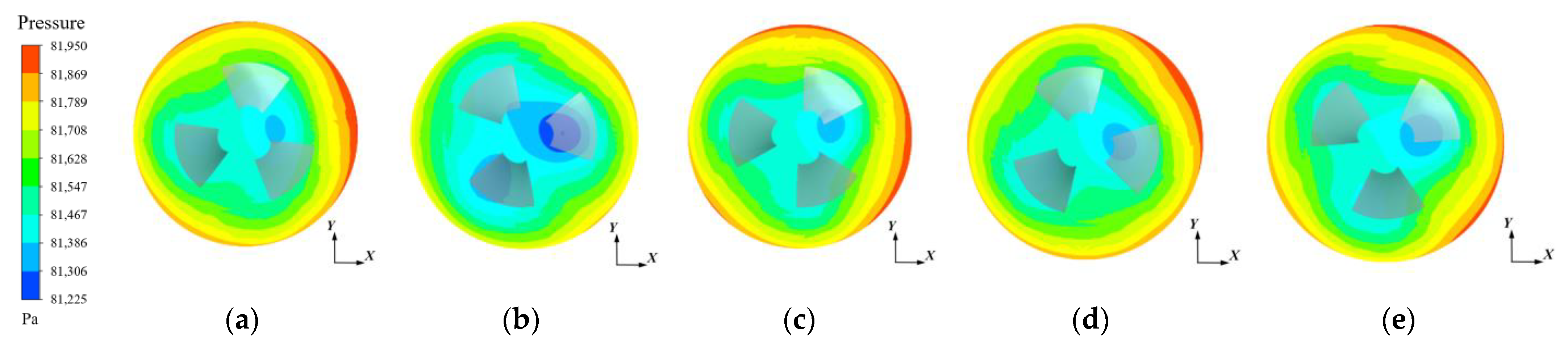
3.3. Flow Pattern at the Bell Mouth
3.4. RAV Formation Mechanism
4. Conclusions
Author Contributions
Funding
Data Availability Statement
Conflicts of Interest
References
- Cristofano, L.; Nobili, M.; Caruso, G. Experimental Study on Unstable Free Surface Vortices and Gas Entrainment Onset Conditions. Exp. Therm. Fluid Sci. 2014, 42, 265–270. [Google Scholar] [CrossRef]
- Andersen, A.; Bohr, T.; Stenum, B.; Rasmussen, J.J.; Lautrup, B. The Bathtub Vortex in a Rotating Container. J. Fluid Mech. 2006, 556, 121–146. [Google Scholar] [CrossRef] [Green Version]
- Trefefthen, L.M.; Bilger, P. The Bath-Tub Vortex in the Southern Hemisphere. Nature 1965, 207, 1084–1085. [Google Scholar] [CrossRef]
- Deeny, D.F. An experimental study of air-entraining vortices at pump sumps. Proc. Inst. Mech. Eng. 1956, 170, 106–116. [Google Scholar] [CrossRef]
- Zhang, D.; Jiao, W.; Cheng, L.; Xia, C.; Zhang, B.; Luo, C.; Wang, C. Experimental study on the evolution process of the roof-attached vortex of the closed sump. Renew. Energy 2021, 164, 1029–1038. [Google Scholar] [CrossRef]
- Sarkardeh, H.; Zarrati, A.R.; Jabbari, E.; Roshan, R. Discussion of “prediction of intake vortex risk by nearest neighbors modeling”. J. Hydraul. Eng. 2012, 138, 374–375. [Google Scholar] [CrossRef]
- Park, I.; Kim, H.J.; Seong, H.; Rhee, D.S. Experimental studies on surface vortex mitigation using the floating anti-vortex device in sump pumps. Water 2018, 10, 441. [Google Scholar] [CrossRef] [Green Version]
- Van Dyke, M. Swirling Flows Vortex Flow in Nature and Technology. Science 1984, 224, 730–731. [Google Scholar] [CrossRef]
- Sarkardeh, H.; Marosi, M. An analytical model for vortex at vertical intakes. Water Supply 2021, 22, 31–43. [Google Scholar] [CrossRef]
- Song, X.J.; Liu, C. Experimental investigation of pressure pulsation induced by the floor-attached vortex in an axial flow pump. Adv. Mech. Eng. 2019, 11, 1687814019838708. [Google Scholar] [CrossRef] [Green Version]
- Song, X.J.; Liu, C. Experimental investigation of floor-attached vortex effects on the pressure pulsation at the bottom of the axial flow pump sump. Renew. Energy 2021, 145, 2327–2336. [Google Scholar] [CrossRef]
- Song, X.J.; Liu, C. Experimental study of the floor-attached vortices in pump sump using V3V. Renew. Energy 2021, 164, 752–766. [Google Scholar] [CrossRef]
- Kang, W.T.; Yu, K.H.; Lee, S.Y.; Shin, B.R. An investigation of cavitation and suction vortices behavior in pump sump. In Proceedings of the Fluids Engineering Division Summer Meeting, Toronto, ON, Canada, 1–3 August 2022. [Google Scholar]
- Pan, Q.; Zhao, R.; Wang, X.; Shi, W.; Zhang, D. LES study of transient behaviour and turbulent characteristics of free-surface and floor-attached vortices in pump sump. J. Hydraul. Res. 2018, 57, 733–743. [Google Scholar] [CrossRef]
- Amin, A.; Kim, B.H.; Kim, C.G.; Lee, Y.H. Numerical Analysis of Vortices Behavior in a Pump Sump. IOP Conf. Ser. Earth Environ. Sci. 2019, 240, 032020. [Google Scholar] [CrossRef]
- Kim, H.J.; Park, S.W.; Rhee, D.S. Effective Height of a Floor Splitter Anti-Vortex Device under Varying Flow Conditions. Sustainability 2017, 9, 285. [Google Scholar] [CrossRef] [Green Version]
- Arocena, V.M.; Abuan, B.E.; Reyes, J.G.T.; Rodgers, P.L.; Danao, L.A.M. Reduction of Entrained Vortices in Submersible Pump Suction Lines Using Numerical Simulations. Energies 2021, 13, 6136. [Google Scholar] [CrossRef]
- Rabe, B.K.; Najafabadi, S.H.G.; Sarkardeh, H. Numerical simulation of air-core vortex at intake. Curr. Sci. 2017, 113, 141–147. [Google Scholar] [CrossRef]
- Tahershamsi, A.; Rahimzadeh, H.; Monshizadeh, M.; Sarkardeh, H. An experimental study on free surface vortex dynamics. Meccanica 2018, 53, 3269–3277. [Google Scholar] [CrossRef]
- Echávez, G.; McCann, E. An experimental study on the free surface vertical vortex. Exp. Fluids 2002, 33, 414–421. [Google Scholar] [CrossRef]
- Cheng, L.; Liu, C.; Zhou, J.; Tang, F.; Yang, H. The study on the flow fields and hydraulic performance in the pump sump. In Proceedings of the 5th Joint ASME/JSME Fluids Engineering Conference, San Diego, CA, USA, 30 July–2 August 2007. [Google Scholar]
- Jiao, W.; Cheng, L.; Zhang, D.; Zhang, B.; Su, Y. Investigation of Key Parameters for Hydraulic Optimization of an Inlet Duct Based on a Whole Waterjet Propulsion Pump System. Trans. FAMENA 2021, 45, 145–162. [Google Scholar] [CrossRef]
- Rajendran, V.P.; Patel, V.C. Measurement of vortices in model pump-intake bay by PIV. J. Hydraul. Eng. 2000, 126, 322–334. [Google Scholar] [CrossRef]
- Constantinescu, S.G.; Patel, V.C. Numerical model for simulation of pump-intake flow and vortices. J. Hydraul. Eng. 1998, 124, 123–134. [Google Scholar] [CrossRef]
- Constantinescu, S.G.; Patel, V.C. Role of turbulence model in prediction of pump-bay vortices. J. Hydraul. Eng. 2000, 126, 387–391. [Google Scholar] [CrossRef]
- Choi, J.W.; Choi, Y.D.; Kim, C.G.; Lee, Y.H. Flow Uniformity in a Multi-Intake Pump Sump Model. J. Mech. Sci. Technol. 2010, 24, 1389–1400. [Google Scholar] [CrossRef]
- Okamura, T.; Kamemoto, K.; Matsui, J. CFD Prediction and Model Experiment on Suction Vortices in Pump Sump. In Proceedings of the 9th Asian International Conference on Fluid Machinery, Jeju, Korea, 16–19 October 2007. [Google Scholar]
- Li, S.; Silva, J.M.; Lai, Y.; Weber, L.J.; Patel, V.C. Three-dimensional simulation of flows in practical water-pump intakes. J. Hydroinformatics 2006, 8, 111–124. [Google Scholar] [CrossRef]
- Jiao, W.; Cheng, L.; Zhang, D.; Zhang, B.; Su, Y.; Wang, C. Optimal Design of Inlet Passage for Waterjet Propulsion System Based on Flow and Geometric Parameters. Adv. Mater. Sci. Eng. 2019, 10, 2320981. [Google Scholar] [CrossRef] [Green Version]
- Jiao, W.; Cheng, L.; Xu, J.; Wang, C. Numerical Analysis of Two-Phase Flow in the Cavitation Process of a Waterjet Propulsion Pump System. Processes 2019, 7, 690. [Google Scholar] [CrossRef] [Green Version]
- Zhang, D.; Cheng, L.; Li, Y.Y.; Jiao, W.X. The hydraulic performance of twin-screw pump. J. Hydrodyn. 2020, 32, 605–615. [Google Scholar] [CrossRef]
- Hunt, J.C.; Wray, A.A.; Moin, P. Eddies, streams, and convergence zones in turbulent flows. Stud. Turbul. Using Numer. Simul. Databases 1988, 2, 193–208. [Google Scholar]
- Dallmann, U. Topological structures of three-dimensional vortex flow separation. In Proceedings of the 16th Fluid and Plasmadynamics Conference, Danvers, MA, USA, 12–14 July 1983; p. 1735. [Google Scholar]
- Liu, C.Q.; Yan, Y.H.; Lu, P. Physics of turbulence generation and sustenance in a boundary layer. Comput. Fluids 2014, 102, 353–384. [Google Scholar] [CrossRef]
- Chong, M.S.; Perry, A.E.; Cantwell, B.J. A general classification of three-dimensional flow fields. Phys. Fluids A Fluid Dyn. 1990, 2, 765–777. [Google Scholar] [CrossRef]


| Parameters | Value |
|---|---|
| Impeller diameter | D = 120 mm |
| Tip clearance | 0.15 mm |
| The ratio of hub and shroud | 0.36 |
| Bell mouth diameter | DL = 190 mm |
| Number of pump blades | Z1 = 3 |
| Impeller speed | n = 2400 r/min |
| Number of guide vanes | Z2 = 5 |
| Number | Number of Grid Cells | Pump Section Head/m |
|---|---|---|
| 1 | 128,265 | 2.39 |
| 2 | 288,222 | 2.37 |
| 3 | 608,565 | 2.37 |
| 4 | 1,087,590 | 2.37 |
| Main Parameters | CFX Settings |
|---|---|
| Flow hypothesis | Incompressible |
| Simulation type | Transient |
| time step | 0.0025 s |
| Total time | 0.25 s |
| Inlet boundary conditions | Mass flow, Q = 36.3 kg/s |
| Outlet boundary conditions | 1 atm |
| Rotational speed | 2400 rev/min |
| Static-static interface | GGI |
| Dynamic-static interface | Transient Rotor Stator |
| Wall condition | Non-slip |
| Wall function | Scalable wall function |
| Convergence accuracy | 10−5 |
Publisher’s Note: MDPI stays neutral with regard to jurisdictional claims in published maps and institutional affiliations. |
© 2022 by the authors. Licensee MDPI, Basel, Switzerland. This article is an open access article distributed under the terms and conditions of the Creative Commons Attribution (CC BY) license (https://creativecommons.org/licenses/by/4.0/).
Share and Cite
Zhang, B.; Cheng, L.; Zhu, M.; Jiao, W.; Zhang, D. Numerical Simulation and Analysis of the Flow Characteristics of the Roof-Attached Vortex (RAV) in a Closed Pump Sump. Machines 2022, 10, 209. https://doi.org/10.3390/machines10030209
Zhang B, Cheng L, Zhu M, Jiao W, Zhang D. Numerical Simulation and Analysis of the Flow Characteristics of the Roof-Attached Vortex (RAV) in a Closed Pump Sump. Machines. 2022; 10(3):209. https://doi.org/10.3390/machines10030209
Chicago/Turabian StyleZhang, Bowen, Li Cheng, Minghu Zhu, Weixuan Jiao, and Di Zhang. 2022. "Numerical Simulation and Analysis of the Flow Characteristics of the Roof-Attached Vortex (RAV) in a Closed Pump Sump" Machines 10, no. 3: 209. https://doi.org/10.3390/machines10030209