Denoising and Feature Extraction for Space Infrared Dim Target Recognition Utilizing Optimal VMD and Dual-Band Thermometry

Abstract

Space target feature extraction and space infrared target recognition are important components of space situational awareness (SSA). However, owing to far imaging distance between the space target and infrared detector, the infrared signal of the target received by the detector is dim and easily contaminated by noise. To effectively improve the accuracy of feature extraction and recognition, it is essential to suppress the noise of the infrared signal. Hence, a novel denoising and extracting feature method combinating optimal variational mode decomposition (VMD) and dual-band thermometry (DBT) is proposed. It takes the mean weighted fuzzy-distribution entropy (FuzzDistEn) of the band-limited intrinsic mode functions (BLIMFs) as the optimization index of dragonfly algorithm (DA) to obtain the optimal parameters (K, α) of VMD. Then the VMD is utilized to decompose the noisy signal to obtain a series of BLIMFs and the Pearson correlation coefficient (PCC) is proposed to determine the effective modes to reconstructe the denoising signal. Finally, based on the denoising signal, the feature of temperature and emissivity-area product are calculated using the DBT. The simulation and experiment results show that the proposed method has better noise reduction performance compared with the other denoising methods, and the accuracy of feature extraction is improved at different noise equivalent irradiance. This provides more accurate feature of temerpature and emissivity-area product for space infrared dim target recognition.

1. Introduction

The research on the infrared radiation characteristics of space targets has attracted extensive attention in many application fields, such as space kill assessment (SKA), space debris monitoring and removal, dim target detection, etc. [1,2,3]. Infrared radiation is not only an important information source for target detection, and recognition, but also an important basis for infrared system design and experiment [4]. Due to the fact that the far imaging distance between the space target and infrared detector, the target usually emerges as only one or several pixels on the infrared image, the infrared signal of the target is dim, and information of target such as shape, attitude, and texture is missing [5,6]. All the information, such as the temperature, emissivity-area product, micromotion, is contained in a few pixels. This brings the possibility of feature extraction, classification, and recognition of space dim targets. However, the factors of the detector system, including temperature variation effect, calibration error of sensor location, photoelectrical noise, seriously interferes with the infrared radiation signal of the space target, resulting in a low signal-to-noise ratio (SNR) of the signal. It restricts the classification and recognition ability of an infrared sensor to a dim and small space target. Therefore, researching a robust denoising model and then extracting accurate features of the infrared signal is of great significance in target classification and recognition.

Currently, many signal denoising methods, including wavelet transform (WT) [7], local projection (LP) [8], singular value decomposition (SVD) [6,9], empirical mode decomposition (EMD) [10], and complete EEMD with adaptive noise (CEEMDAN) [11] have been applied to suppress noise. However, these methods have varying degrees of limitations. The effect of the WT relies on the preset value of the wavelet basis, decomposition level, and wavelet threshold; the denoising performance of the LP method is closely related to the selection of neighborhood radius; the SVD method needs to overcome the problem that how to determine the cutting point of singular value array. EMD has the limitations of mode mixing, noise sensitivity, and endpoint effects. CEEMDAN produce error accumulation and lack rigorous mathematical theory for support.

Variational mode decomposition (VMD) was proposed by Dragomiretskiy and had shown excellent performance in solving mode mixing and endpoint effects [12]. It was established based on the Wiener filtering, Hilbert transform, and frequency shifting. According to the alternative direction multiplier method, it can estimate multiple modes with different center frequencies and bandwidths simultaneously in a non-recursive manner. Many studies have focused more attention on the VMD method, including ionospheric scintillation effects on GNSS, the extraction of weak features, the denoising of Load signal, and others [13,14,15,16]. However, the VMD is rarely applied to the denoising of infrared signals. The performance of VMD is strongly restricted by the decomposition modes number $\mathrm{K}$ and the penalty factor $\mathsf{\alpha }$. If the unreasonable value of $\mathrm{K}$ and $\mathsf{\alpha }$ is selected, it may lend to discarding important modes or producing mixing intrinsic mode functions (IMFs). The relationship between the result of decomposing signal and the two values is as follows [17]: (1) When the K value is too small: it may lead to some modes being shared under small $\mathsf{\alpha }$, resulting in information redundancy, conversely, some effective modes will be discarded under a large $\mathsf{\alpha }$. (2) When the K value is too large, the characteristic of some modes is similar to white noise under a small $\mathsf{\alpha }$, instead, duplicate modes will be produced (3) When the K value is proper, there is a high possibility that the method doesn’t converge to the true central frequencies for higher $\mathsf{\alpha }$.

To solve the problem of selecting the parameters K and α, many researchers have carried out considerable work to address it. Liu et al. combined variational mode decomposition and detrend fluctuation analysis (DFA) to select decomposition layers K [18]. Li et al. determined the K value by calculating the maximum frequency difference of different IMFs to judge whether the decomposition is excessive; however, the range of judging criterion cannot be adaptive [19]. With help of six indicators, Lian et al. proposed a comprehensive model to identify the optimal value of K [20]. Theoretically, it can perfectly prevent overbinning and underbinning. However, it is apparent that the thresholds of indicators are difficult to determine and the adaptivity is in constraint.

With the development of optimization algorithms, some researchers have determined the VMD parameters adaptively by using them to optimize the fitness function. Anil et al. optimized kernel-based mutual information (KEMI) fitness function by applying a genetic algorithm (GA) to obtain the decomposition parameters combination of VMD [15]. Li et al. optimized the VMD parameters by taking the local maximum envelope peakfactor as the fitness function of particle swarm optimization (PSO) and determined the optimal combination [21]. However, these algorithms are proved to have relatively slow convergence speed in the search space and may not be able to achieve the optimal value. This paper employs a novel meta-heuristic optimization algorithm called the dragonfly algorithm (DA), which was proposed by Seyedali Mirjalili, to search the global optimal value effectively and efficiently [22]. The algorithm is inspired by dragonflies in nature. The most important procedurs, exploration and exploitation [23], are designed by modeling separation, alignment, and cohesion motions of dragonflies to achieve the purpose of survival. The experiment shows that this algorithm can rapidly converge and provide highly competitive results compared to PSO. Thus, these advantages prove it is preferable to use the DA for VMD optimization and denoising.

Due to different heat capacities, materials, size and micromotion of space targets, they show different the change of temperature and the emissivity-area product [24]. In this paper, the two featuers are the concerning features. The emissivity-area product can be calculated from the radiation characteristics, assuming that the distance and temperature of the target are known. Therefore, how to obtain the target temperature accurately is important. Radiation temperature measurement can be utilized to obtain the temperature. It can be classified single-band thermometry(ST), dual-band thermometry (DBT), and multiband thermometry (MT) according to the number of infrared bands [25,26,27]. ST is the most common method in the infrared radiation system. However, the measured radiation includes the self-radiation of the target and the reflected external radiation, the method can only obtain the brightness temperature of the target. MT is used to obtain the surface temperature and emissivity of the target through the combination of target radiation and emissivity model. However, if there is a great difference between the set emissivity model and the actual model of the target, the temperature measurement accuracy decreases sharply. Assuming target is gray, DBT gathers the radiation energy of the target in two different bands through the detector and calculates the temperature of the target according to the radiation ratio. Compared with ST, the method can eliminate the influence of target emissivity on target temperature measurement to a certain extent and improve the temperature measurement accuracy. Compared with MT, the method does not require more hypothetical information.

To solve denoising, improve the accuracy of feature extraction and provide preliminary design indications (such as the infrared bands selection, the values of equivalent noise irradiance (NEI), etc.) for the machine and structure of the payload system on satellite before manufacturing, so as to get the ideal payload more efficiently and quickly, this paper proposes a new method combining the VMD algorithm with DA and DBT. The remainder of this paper is depicted as follows: In Section 2, the principle and steps of DA are introduced in detail. Also, the VMD algorithm and DBT will also be presented. Section 3 introduces and discusses the denoising and extracting feature procedures for the infrared signal. In Section 4, firstly, simulation parameters are set, then the performance of the DA-VMD is compared with the other four common denoising methods. Lastly, DBT is used to extract features of the denoising signal results of the DA-VMD. In Section 5, the measured data based semi-physical simulation platform further proves the feasibility and effectiveness of the proposed DA-VMD-DBT. Finally, in Section 6, the conclusion of this paper is drawn, and future work is envisioned and proposed.

2. Theoretical Background

2.1. Dragonfly Algorithm Description

The dragonfly algorithm (DA)—proposed by Mirjalili—is a new meta-heuristic optimization technique. The algorithm mimics the behavior of dragonflies in nature. For dragonflies’ swarms, they mainly three primitive behavioral principles: separation, alignment, and aggregation. Aside from the above behaviors, attracting food and distracting outward enemies are essential behaviors for individual dragonflies. Therefore, five main factors are considered in the process of optimizing individual positions. Each behavior is expressed as follows:

The separation motion is modeled as follows:

$${\mathrm{S}}_{\mathrm{i}}=-{\displaystyle \sum }_{\mathrm{j}=1}^{\mathrm{N}}\mathrm{X}-{\mathrm{X}}_{\mathrm{j}}$$

(1)

where ${\mathrm{S}}_{\mathrm{i}}$ is the separation metric of the ith individual, $\mathrm{X}$ represents the position of the current individual. ${\mathrm{X}}_{\mathrm{j}}$ means the position of the jth individual, and $\mathrm{N}$ is the number of neighboring individuals.

The alignment motion is calculated as follows:

$${\mathrm{A}}_{\mathrm{i}}=\frac{{{\displaystyle \sum }}_{\mathrm{j}=1}^{\mathrm{N}}{\mathrm{V}}_{\mathrm{j}}}{\mathrm{N}}$$

(2)

where ${\mathrm{A}}_{\mathrm{i}}$ is the alignment metric of the ith individual, ${\mathrm{V}}_{\mathrm{j}}$ shows the velocity of the jth neighboring individual.

The cohesion motion is modeled as follows:

$${\mathrm{C}}_{\mathrm{i}}=\frac{{{\displaystyle \sum }}_{\mathrm{j}=1}^{\mathrm{N}}{\mathrm{X}}_{\mathrm{j}}}{\mathrm{N}}-\mathrm{X}$$

(3)

where ${\mathrm{C}}_{\mathrm{i}}$ is the cohesion metric of the ith individual, $\mathrm{X}$ is the position of the current individual, $\mathrm{N}$ is the number of neighborhoods, and ${\mathrm{X}}_{\mathrm{j}}$ shows the position of the jth neighboring individual.

The motion of attracting towards food for dragonflies is represented as follows:

$${\mathrm{F}}_{\mathrm{i}}={\mathrm{X}}^{+}-\mathrm{X}$$

(4)

where ${\mathrm{F}}_{\mathrm{i}}$ is the attraction food metric of the $\mathrm{i}$th individual, $\mathrm{X}$ is the position of the current individual, and ${\mathrm{X}}^{+}$ shows the location of the food source.

The motion of distracting outward enemies is modeled as follows:

$${\mathrm{E}}_{\mathrm{i}}{=\mathrm{X}}^{-}+\mathrm{X}$$

(5)

where ${\mathrm{E}}_{\mathrm{i}}$ is the distracting metric of the $\mathrm{i}$th individual, $\mathrm{X}$ is the position of the current individual, and ${\mathrm{X}}^{-}$ shows the location of enemies.

Here, to optimize the position of dragonflies in search space and imitate their movements, the step vector $\Delta \mathrm{X}$ is defined to indicate the direction of the movement, its mathematical model is:

$$\Delta {\mathrm{X}}_{\mathrm{t}+1}{=(\mathrm{sS}}_{\mathrm{i}}{+\mathrm{aA}}_{\mathrm{i}}{+\mathrm{cC}}_{\mathrm{i}}{+\mathrm{fF}}_{\mathrm{i}}{+\mathrm{eE}}_{\mathrm{i}})+\mathrm{w}\Delta {\mathrm{X}}_{\mathrm{t}}$$

(6)

where $\mathrm{s}$, $\mathrm{a}$, $\mathrm{c}$, $\mathrm{f}$, and $\mathrm{e}$ indicate the separation weight, alignment weight, cohesion weight, the food factor, the enemy factor, and $\mathrm{w}$ is the inertia weight, $\mathrm{t}$ is the current iteration number. The value of these weights are as follows:

$$\begin{gathered} \mathrm{s},\mathrm{a},\mathrm{c}=2\times \mathrm{rand}\times \max (0,0.1-\frac{0.2\times \mathrm{t}}{\max -\mathrm{iteration}}) \\ \mathrm{f}=2\times \mathrm{rand} \\ \mathrm{e}=0.1-\frac{0.2\times \mathrm{t}}{\max -\mathrm{iteration}} \\ \mathrm{w}=0.9-\frac{(0.9-0.4)\times \mathrm{t}}{\max -\mathrm{iteration}} \end{gathered}$$

(7)

where the max-iteration is the total number of iterations. After obtaining the $\Delta \mathrm{X}$, the position vector can be regarded as:

$${\mathrm{X}}_{\mathrm{t}+1}{=\mathrm{X}}_{\mathrm{t}}+\Delta {\mathrm{X}}_{\mathrm{t}+1}$$

(8)

By changing the above motion weight, different optimization processes can be achieved. The neighborhood radius r of dragonflies is quite important for balancing exploration and exploitation of the entire process, which is depended by the range of parameters to be optimized and the number of iterations. Considering improving the randomness, the random walk (Lévy flight) is used to guarantee some dragonflies to fly over the search space under no neighboring individual. In this situation, the position of dragonflies can be modeled as follows:

$${\mathrm{X}}_{\mathrm{t}+1}{=\mathrm{X}}_{\mathrm{t}}{+\mathrm{L}é\mathrm{vy}\left(\mathrm{d}\right)\times \mathrm{X}}_{\mathrm{t}}$$

(9)

where $\mathrm{t}$ is the iteration number, and $\mathrm{d}$ is the dimension of the position vector. The Lévy flight is represented as:

$$\mathrm{L}é\mathrm{vy}\left(\mathrm{x}\right)=0.01\times \frac{{\mathrm{r}}_1\times \mathsf{\sigma }}{{\left|{\mathrm{r}}_2\right|}^{\frac{1}{\mathsf{\beta }}}}$$

(10)

where ${\mathrm{r}}_1$, ${\mathrm{r}}_2$ are two random numbers in $\left[0,1\right]$, $\mathsf{\beta }$ is a constant value (=1.5), and $\mathsf{\sigma }$ is equal to

$$\mathsf{\sigma }={\left(\frac{\mathsf{\Gamma }(1+\mathsf{\beta })\times \sin \left(\frac{\mathsf{\pi }\mathsf{\beta }}{2}\right)}{\mathsf{\Gamma }(\frac{1+\mathsf{\beta }}{2}{)\times \mathsf{\beta }\times 2}^{\left(\frac{\mathsf{\beta }-1}{2}\right)}}\right)}^{\frac{1}{\mathsf{\beta }}}$$

(11)

where $\mathsf{\Gamma }\left(\mathrm{x}\right)=(\mathrm{x}-1)!$. The pseudo-codes of the DA are depicted in below Algorithm 1.

Algorithm 1 The Pseudo-code of the DA [22].

Initialize the dragonflies population Xi(i = 1, 2, …, n);

Initialize the step vectors ∆Xi(i = 1, 2, …, n);

while the end condition is not satisfied do

Calculate the objective values of all dragonflies

Update the food source and enemy

Update w, s, a, c, f, and e

Calculate S, A, C, F, and E using Equations (1)–(5)

Update neighboring radius r

if a dragonfly has at least one neighboring dragonfly then

Update velocity vector using Equation (6)

Update position vector using Equation (7)

else

Update position vector using Equation (8)

end if

Check and correct the new positions based on the boundaries of variables

end while

2.2. Variational Mode Decomposition

Variational mode decomposition is a new multi-resolution non-recursive signal adaptive decomposition estimator method. Combining Wiener filtering, Hilbert transform, and alternating direction method of multipliers [28], it uses an iterative procedure to obtain the optimal solution and can adaptively decompose the original signal sequence into $\mathrm{K}$ bandwidth-limited IMF functions (namely BLIMFs) around the estimated center frequency ${\mathrm{w}}_{\mathrm{k}}$. The BLIMFs can be expressed as:

$${\mathrm{u}}_{\mathrm{k}}\left(\mathrm{t}\right){=\mathrm{A}}_{\mathrm{k}}\left(\mathrm{t}\right)\cos ({\mathsf{\varphi }}_{\mathrm{k}}\left(\mathrm{t}\right))$$

(12)

where ${\mathrm{A}}_{\mathrm{k}}\left(\mathrm{t}\right)$ and ${\mathsf{\varphi }}_{\mathrm{k}}\left(\mathrm{t}\right)$ denote the envelope and the phase, respectively. Generally, the algorithm is mainly composed of two procedures of constructing variational problems and solving them. The first is to construct the variational problem to estimate the center frequency and bandwidth for BLIMFs. The Hilbert transform is used to obtain a unilateral frequency spectrum of the associated analytic signal of each ${\mathrm{u}}_{\mathrm{k}}$, the BLIMF’s frequency spectrum is shifted to baseband for each ${\mathrm{u}}_{\mathrm{k}}$. The demodulated signal bandwidth is estimated by the Gaussian smoothness, i.e., the squared norm. Based on the above, this problem can be formulated as the following constrained variational problem:

$$\min \left\{{\displaystyle \sum }_{\mathrm{k}=1}^{\mathrm{K}}\Vert \mathsf{\partial }\mathrm{t}\left[\left(\mathsf{\delta }\left(\mathrm{t}\right)+\frac{\mathrm{j}}{\mathsf{\pi }\mathrm{t}}\right){\ast \mathrm{u}}_{\mathrm{k}}\left(\mathrm{t}\right)\right]{\mathrm{e}}^{{-\mathrm{jw}}_{\mathrm{k}}\mathrm{t}}\Vert \begin{array}{c}2\\ 2\end{array}\right\}\mathrm{s}.\mathrm{t}.{\displaystyle \sum }_{\mathrm{k}=1}^{\mathrm{K}}{\mathrm{u}}_{\mathrm{k}}=\mathrm{f}$$

(13)

where ${\mathrm{u}}_{\mathrm{k}}$ represents the $\mathrm{k}$th BLIMF, ${\mathrm{w}}_{\mathrm{k}}$ is the center frequency of ${\mathrm{u}}_{\mathrm{k}}$, $\partial \mathrm{t}$ represents derivative operator and $\mathsf{\delta }\left(\mathrm{t}\right)$ is the Dirac function, $\ast$ represents the convolution operation, and $\mathrm{f}$ is the original signal.

The second is to solve the above variational problem. The Lagrangian multiplier $\mathsf{\lambda }$ and quadratic penalty term $\mathsf{\alpha }$ are introduced to convert the abovementioned problem into an unconstrained variational problem and find the optimal answer. The augmented Lagrangian is expressed as follows:

$$\left({\mathrm{u}}_{\mathrm{k}}{,\mathrm{w}}_{\mathrm{k}},\mathsf{\lambda }\right)=\mathsf{\alpha }\left\{{\displaystyle \sum }_{\mathrm{k}=1}^{\mathrm{K}}\Vert \mathsf{\partial }\mathrm{t}\left[\left(\mathsf{\delta }\left(\mathrm{t}\right)+\frac{\mathrm{j}}{\mathsf{\pi }\mathrm{t}}\right){\ast \mathrm{u}}_{\mathrm{k}}\left(\mathrm{t}\right)\right]{\mathrm{e}}^{{-\mathrm{jw}}_{\mathrm{k}}\mathrm{t}}\Vert \begin{array}{c}2\\ 2\end{array}\right\}+\Vert \mathrm{f}\left(\mathrm{t}\right)-{\displaystyle \sum }_{\mathrm{k}=1}^{\mathrm{K}}{\mathrm{u}}_{\mathrm{k}}\left(\mathrm{t}\right){\Vert }_2^2+<\mathsf{\lambda }\left(\mathrm{t}\right),\mathrm{f}\left(\mathrm{t}\right)-{\displaystyle \sum }_{\mathrm{k}=1}^{\mathrm{K}}{\mathrm{u}}_{\mathrm{k}}\left(\mathrm{t}\right)>$$

(14)

then the alternate direction method of multipliers (ADMM) is used to find the saddle point as the solution of Equation (13), and update ${\mathrm{u}}_{\mathrm{k}}^{\mathrm{n}+1}$, ${\mathrm{w}}_{\mathrm{k}}^{\mathrm{n}+1}$ in frequency, respectively. The iteration equations are as follows:

$${\mathrm{u}}_{\mathrm{k}}^{\mathrm{n}+1}\left(\mathrm{w}\right)=\frac{\hat{\mathrm{f}}\left(\mathrm{w}\right)-{{\displaystyle \sum }}_{\mathrm{i}\ne \mathrm{k}}{\mathrm{u}}_{\mathrm{i}}\left(\mathrm{w}\right)+\frac{\lambda \left(\mathrm{w}\right)}{2}}{1+2\alpha {(\mathrm{w}-{\mathrm{w}}_{\mathrm{k}})}^2}$$

(15)

$${\mathrm{w}}_{\mathrm{k}}^{\mathrm{n}+1}=\frac{{{\displaystyle \int }}_0^{\infty }\mathrm{w}{\left|{\mathrm{u}}_{\mathrm{k}}\left(\mathrm{w}\right)\right|}^2\mathrm{dw}}{{{\displaystyle \int }}_0^{\infty }{\left|{\mathrm{u}}_{\mathrm{k}}\left(\mathrm{w}\right)\right|}^2\mathrm{dw}}$$

(16)

The iterative process is repeated according to the above equations until the convergence stop condition is satisfied.

$${\displaystyle \sum }_{\mathrm{k}}\Vert {\mathrm{u}}_{\mathrm{k}}^{\mathrm{n}+1}{-\mathrm{u}}_{\mathrm{k}}^{\mathrm{n}}{\Vert }_2^2{/\Vert \mathrm{u}}_{\mathrm{k}}^{\mathrm{n}}{\Vert }_2^2<\mathsf{ϵ}$$

(17)

The parameter $\mathsf{ϵ}$ of VMD is tolerance of convergence criterion. In this paper, the value is set as ${10}^{-7}$. Based on the above steps, the VMD algorithm is executed as follows:

Step 1: Initialize the parameters ${\mathrm{u}}_{\mathrm{k}}^1$, ${\mathrm{w}}_{\mathrm{k}}^1$, $\mathrm{K}$. $\mathrm{K}$ is the predefined number of decomposed modes;

Step 2: Execute the loop to update the $\mathrm{K}$ BLIMFs in the spectral domain ${\mathrm{u}}_{\mathrm{k}}^{\mathrm{n}+1}\left(\mathrm{w}\right)$ based on Equation (15);

Step 3: Execute the loop to update the center frequencies ${\mathrm{w}}_{\mathrm{k}}^{\mathrm{n}+1}$ of all BLIMFs based on Equation (16).

Step 4: Repeat the algorithm from Steps 2 to 3 until the convergence stop condition is satisfied.

3. Methodology

This section will first introduce the concept of DA-VMD parameter optimization, including the fitness function and the relevant modes. Then, DBT is utilized to extract temperature and the emissivity-area product, considering external radiation. Finally, the detailed steps of the proposed method DA-VMD-DBT are given.

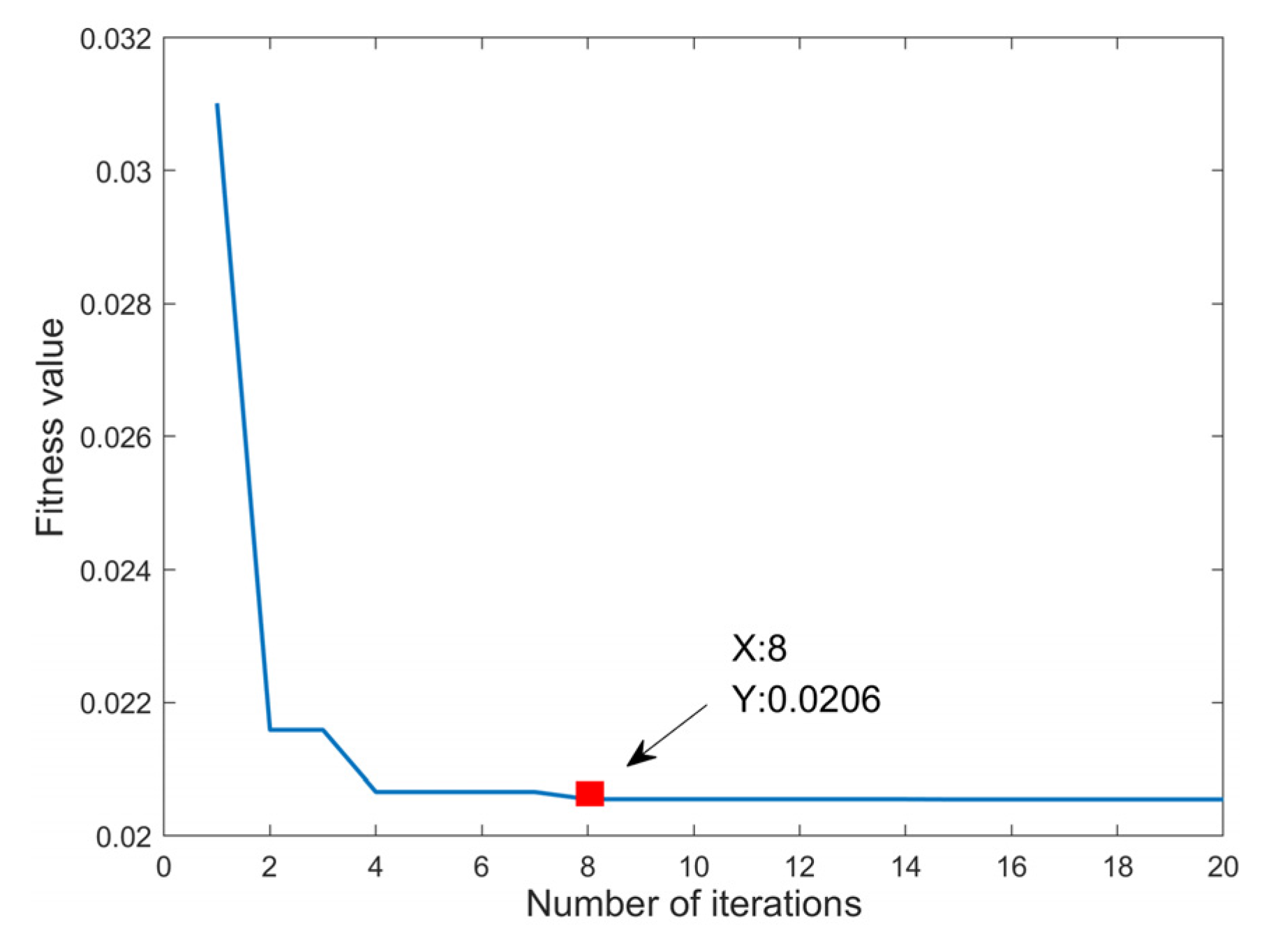
3.1. DA-VMD Parameter Optimization

Although the principle of VMD indicates that VMD can overcome the mode mixing caused by EMD, based on the above statement, it is known that the denoising result of VMD is restricted by the decomposition mode $\mathrm{K}$ and the penalty factor $\mathsf{\alpha }$. To solve the problem, we propose adopting the DA to decide the parameters.

(1)

Fitness function construction

Before the DA is used to optimize the parameters K and α, the fitness function must be determined to evaluate the parameters. Entropy is a measure of the chaos of the dynamic characteristics in a system or signal. In this paper, the mean weighted fuzzy distribution entropy (FuzzDistEn) is constructed as the objective function in VMD parameter optimization [29]. It not only combines the advantages of good robustness of distribution entropy and the fuzzy membership function of fuzzy entropy but also considers the correlation between the decomposition sequences and the noisy infrared signal sequence. Hence, the mean weighted FuzzDistEn has great potential in VMD optimization.

During the processing of the infrared signal by the VMD algorithm, if there is no modal aliasing, decomposition modes are clear and determined, and the mean weighted FuzzDistEn is smaller, which is preferred. Otherwise, the energy distribution in decomposition sequences will be complex and undermined, and the value of the mean weighted FuzzDistEn is larger. Therefore, during the optimization process of the DA, the two parameter values of $\mathrm{K}$ and $\mathsf{\alpha }$ corresponding to the minimum mean weighted FuzzDistEn are the final optimization result. The steps of the fitness function are described as follows:

Step 1: Reconstruct the state space vectors and construct the distance matrix. For $\mathrm{i}$th component of BLIMFs $\mathrm{u}\left(\mathrm{i}\right)=\left\{\mathrm{u}\left(1\right),\mathrm{u}\left(2\right),\cdots \mathrm{u}\left(\mathrm{n}\right)\right\}$, the state space vectors are formed:

$${\mathrm{X}}_{\mathrm{i}}^{\mathrm{m}}=\left\{\mathrm{u}\left(\mathrm{i}\right),\mathrm{u}\left(\mathrm{i}+1\right),\cdots \mathrm{u}\left(\mathrm{i}+\mathrm{m}-1\right)\right\}{-\mathrm{u}}_0\left(\mathrm{i}\right),\mathrm{i}=1,2,\dots \mathrm{N}-\mathrm{m}+1$$

(18)

where $\mathrm{m}$ is the embedding dimension and ${\mathrm{u}}_0\left(\mathrm{i}\right)$ represents the baseline of the ith vector.

Then, the distance matrix ${\mathrm{d}}_{\mathrm{ij}}^{\mathrm{m}}$ between ${\mathrm{X}}_{\mathrm{i}}^{\mathrm{m}}$ and ${\mathrm{X}}_{\mathrm{j}}^{\mathrm{m}}$ is calculated as:

$${\mathrm{d}}_{\mathrm{ij}}^{\mathrm{m}}=\mathrm{d}\left[{\mathrm{X}}_{\mathrm{i}}^{\mathrm{m}}{,\mathrm{X}}_{\mathrm{j}}^{\mathrm{m}}\right]{=\max }_{\mathrm{k}}\left\{\left|\mathrm{u}\left(\mathrm{i}+\mathrm{k}\right)-\mathrm{u}\left(\mathrm{j}+\mathrm{k}\right)\right|\right\} \left(1⩽\mathrm{i},\mathrm{j}⩽\mathrm{N}-\mathrm{m}+1,0⩽\mathrm{k}⩽\mathrm{m}-1,\mathrm{i}\ne \mathrm{j}\right)$$

(19)

where $\mathrm{k}$ is the order of elements, and it is noted that ${\mathrm{d}}_{\mathrm{ij}}^{\mathrm{m}}$ is an asymmetrical matrix.

Step 2: Calculate the similarity degree ${\mathrm{D}}_{\mathrm{ij}}^{\mathrm{m}}$ based on the fuzzy function ${\mathrm{f}(\mathrm{d}}_{\mathrm{ij}}^{\mathrm{m}},\mathrm{n},\mathrm{r})$, as per the following equations:

$$\{\begin{array}{c}{\mathrm{D}}_{\mathrm{ij}}^{\mathrm{m}}{=\mathrm{f}(\mathrm{d}}_{\mathrm{ij}}^{\mathrm{m}},\mathrm{n},\mathrm{r})\\ \mathrm{f}\left({\mathrm{d}}_{\mathrm{ij}}^{\mathrm{m}},\mathrm{n},\mathrm{r}\right)=\exp (-{\left({\mathrm{d}}_{\mathrm{ij}}^{\mathrm{m}}\right)}^{\mathrm{n}}/\mathrm{r})\end{array}$$

(20)

where $\mathrm{r}$ denotes the predetermined tolerance and $\mathrm{n}$ is the order of the exponential function. In this paper, the value of $\mathrm{r}$ is set to $0.20\times \mathrm{std}\left(\mathrm{u}\right(\mathrm{i}\left)\right)$, $\mathrm{n}$ is equal to 2.

Step 3: Calculate the estimate probability density and FuzzDistEn. Following the procedure of probability density estimation of DistEn [30], the empirical probability density function (ePDF) $\mathrm{Pt}$ of ${\mathrm{D}}_{\mathrm{ij}}^{\mathrm{m}}$ is calculated. Then, the normalized FuzzDistEn is calculated as:

$$\mathrm{FuzzDistEn}(\mathrm{M},\mathrm{m},\mathrm{n},\mathrm{r})=-\frac{1}{{\log }_2\mathrm{M}}{\displaystyle \sum }_{\mathrm{t}=1}^{\mathrm{M}}\mathrm{Pt}·{\log }_2\mathrm{Pt}$$

(21)

where $\mathrm{M}$ is the number of bins of the histogram, and $\mathrm{m}$ is the embedding dimension.

Step 4: Calculate the mutual information. The mutual information between BLIMF and the original signal $\mathrm{Y}$ can be defined as:

$$\mathrm{I}(\mathrm{u};\mathrm{Y})={\displaystyle \sum }_{\mathrm{u}}{\displaystyle \sum }_{\mathrm{Y}}\mathrm{p}(\mathrm{u},\mathrm{Y})\log \frac{\mathrm{p}(\mathrm{u},\mathrm{Y})}{\mathrm{p}\left(\mathrm{u}\right)\mathrm{p}\left(\mathrm{Y}\right)}$$

(22)

where $\mathrm{p}\left(\mathrm{u}\right)$, $\mathrm{p}\left(\mathrm{Y}\right)$, and $\mathrm{p}(\mathrm{u},\mathrm{Y})$ represent the edge probability distribution and the joint probability distribution of $\mathrm{u}$ and $\mathrm{Y}$, respectively.

Step 5: Calculate the mean weighted FuzzDistEn of IMFs as:

$$\mathrm{mean}\mathrm{weighted}\mathrm{FuzzDistEn}=\frac{{{\displaystyle \sum }}_{\mathrm{i}=1}^{\mathrm{N}}\mathrm{FuzzDistEn}\left(\mathrm{u}\right(\mathrm{i}\left)\right)\cdot \mathrm{I}\left(\mathrm{u}\right(\mathrm{i});\mathrm{Y})}{\mathrm{N}}$$

(23)

where $\mathrm{u}\left(\mathrm{i}\right)$ represents the decomposition modes, $\mathrm{N}$ is the IMF number.

(2)

Related modes selection method

According to the above-mentioned principle of the VMD algorithm, the original noisy signal can be decomposed into several BLIMFs from low to high frequency by using the VMD algorithm. How to select these BLIMFs will directly determine the final noise reduction effect. In general, the random noise is mainly distributed in the high-frequency phase and the effective signal is concentrated in the low-frequency phase. To more effectively reduce components by using the VMD algorithm, it is necessary to find the demarcation point between the noise BLIMF components (irrelevant modes) and the effective BLIMF components (relevant modes). In statistics, the Pearson correlation coefficient [31] (PCC) can be used to estimate the correlation between two vectors X and Y, and its value is between −1 and 1. Thus, we use the measurement criterion to select the effective BLIMFs. It is defined as follows:

$$\rho (\mathrm{i})=\frac{\mathrm{cov}\left(\mathrm{u}\left(\mathrm{i}\right),\mathrm{Y}\right)}{{\mathsf{\sigma }}_{\mathrm{u}\left(\mathrm{i}\right)}{\mathsf{\sigma }}_{\mathrm{Y}}}=\frac{\mathrm{E}\left(\mathrm{u}\left(\mathrm{i}\right),\mathrm{Y}\right)-\mathrm{E}\left(\mathrm{u}\left(\mathrm{i}\right)\right)\mathrm{E}\left(\mathrm{Y}\right)}{\sqrt{\mathrm{E}\left({\mathrm{u}\left(\mathrm{i}\right)}^2\right)-{\mathrm{E}}^2\left(\mathrm{u}\left(\mathrm{i}\right)\right)}\sqrt{\mathrm{E}\left({\mathrm{Y}}^2\right)-{\mathrm{E}}^2\left(\mathrm{Y}\right)}}=\frac{{\displaystyle \sum }(\mathrm{u}\left(\mathrm{i}\right)-\overline{\mathrm{u}\left(\mathrm{i}\right)})(\mathrm{Y}-\overline{\mathrm{Y}})}{\sqrt{{\displaystyle \sum }({\mathrm{u}\left(\mathrm{i}\right)-\overline{\mathrm{u}\left(\mathrm{i}\right)})}^2}\sqrt{{\displaystyle \sum }{(\mathrm{Y}-\overline{\mathrm{Y}})}^2}}$$

(24)

where $\mathrm{u}\left(\mathrm{i}\right)$ is the $\mathrm{i}$th BLIMF and $\mathrm{Y}$ is the infrared signal. The greater the value of the PCC, the stronger correlation between $\mathrm{u}\left(\mathrm{i}\right)$ and $\mathrm{Y}$. Based on the above, the demarcation point $\mathrm{k}$ of the effective BLIMFs and the noise BLIMFs can be determined by the following formula:

$$\mathrm{k}=\arg \underset{1\le \mathrm{i}\le \mathrm{K}-1}{\max }\left|\mathrm{diff}\left(\mathsf{\rho }\left(\mathrm{i}\right)\right)\right|$$

(25)

and the reconstitution signal $\stackrel{\sim }{\mathrm{y}}$ can be obtained as follows:

$$\stackrel{\sim }{\mathrm{y}}={\displaystyle \sum }_{\mathrm{i}=1}^{\mathrm{k}+1}{\mathrm{BLIMF}}_{\mathrm{i}}$$

(26)

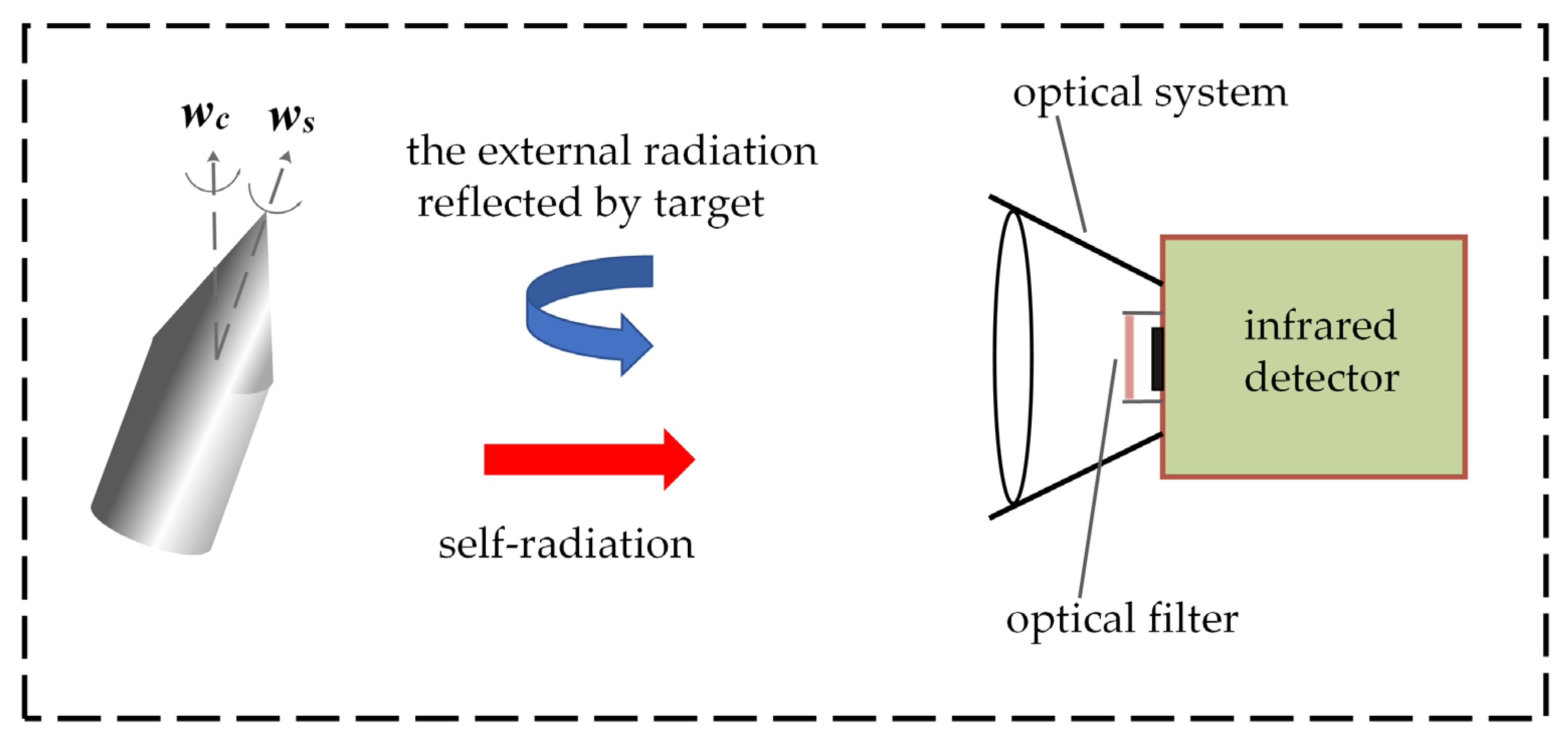
3.2. Target Temperature and Emissivity-Area Product Feature Extraction Based on DBT

Temperature is an important parameter to characterize the state of matter. It plays an important role in security, scientific experiments, and agricultural production. Emitting radiation is affected by the temperature and material of the target, and the relationship between radiation and temperature can be evaluated by Plank’s law [32]. With the help of an infrared detector, the radiation of target can be calculated from the generated multi-frame infrared images. Then the temperature distribution of target can be obtained from the inversion of radiation. We have established a radiation diagram from the space target to the infrared detector, as shown in Figure 1. Since that the background of the target is a deep space background, its background radiation is ignored. The external radiation mainly considers the following three parts: the solar radiation ${\mathrm{L}}_{\mathrm{rs}}$, the Earth radiation ${\mathrm{L}}_{\mathrm{re}}$, and the solar radiation reflected by Earth ${\mathrm{L}}_{\mathrm{res}}$. So there are two main radiation sources at the entrance pupil of the detector: the self-radiation of the target and the external radiation reflected by the target. In this paper, we consider the influence of external radiation on the radiation temperature measurement, which changes the previous situation of temperature measurement only considering self-radiation. To describe the relationship between detector and space targets temperature, the following simplifications are assumed: the emissivity of the target surface is constant; the path transmittance is one, and the detector receives all radiation within a band.

To simplify, we use the equivalent radiance $\left(1-{\mathsf{ϵ}}_{\mathrm{s}}\right){{\displaystyle \int }}_{{\mathsf{\lambda }}_1}^{{\mathsf{\lambda }}_2}{\mathrm{L}}_{\mathsf{\lambda }}\left({\mathrm{T}}_{\mathrm{a}}\right)\mathrm{d}\mathsf{\lambda }$ to describe the total external radiance reflected by the target, as follows:

$$\left(1-{\mathsf{ϵ}}_{\mathrm{s}}\right){{\displaystyle \int }}_{{\mathsf{\lambda }}_1}^{{\mathsf{\lambda }}_2}{\mathrm{L}}_{\mathsf{\lambda }}\left({\mathrm{T}}_{\mathrm{a}}\right)\mathrm{d}\mathsf{\lambda }=\left(1-{\mathsf{ϵ}}_{\mathrm{s}}\right){{\displaystyle \int }}_{{\mathsf{\lambda }}_1}^{{\mathsf{\lambda }}_2}{(\mathrm{L}}_{\mathrm{rs}}{+\mathrm{L}}_{\mathrm{re}}{+\mathrm{L}}_{\mathrm{res}})\mathrm{d}\mathsf{\lambda }$$

(27)

where ${\mathsf{ϵ}}_{\mathrm{s}}$ is the emissivity of the target surface material, ${\mathsf{\lambda }}_1$ and ${\mathsf{\lambda }}_2$ is the cutoff wavelength.

${\mathrm{L}}_{\mathrm{rs}}$ is the solar radiation radiance, ${\mathrm{L}}_{\mathrm{re}}$ is the radiant radiance of the Earth, ${\mathrm{L}}_{\mathrm{res}}$ is the radiance of solar radiation reflected by Earth.

The output signal of the detector is usually proportional to the thermal radiation absorbed by the infrared focal plane. Based on the above statements, the image gray value corresponding to the target can be calculated by the following formula:

$$\mathrm{S}=\mathrm{K}\mathsf{\tau }\mathrm{A}\left[{\mathsf{ϵ}}_{\mathrm{s}}{{\displaystyle \int }}_{{\mathsf{\lambda }}_1}^{{\mathsf{\lambda }}_2}{\mathrm{L}}_{\mathsf{\lambda }}\left({\mathrm{T}}_{\mathrm{s}}\right)\mathrm{d}\mathsf{\lambda }+\left(1-{\mathsf{ϵ}}_{\mathrm{s}}\right){{\displaystyle \int }}_{{\mathsf{\lambda }}_1}^{{\mathsf{\lambda }}_2}{\mathrm{L}}_{\mathsf{\lambda }}\left({\mathrm{T}}_{\mathrm{a}}\right)\mathrm{d}\mathsf{\lambda }\right]{/(\mathsf{\pi }\mathrm{R}}^2)+\mathrm{b}$$

(28)

where $\mathrm{S}$ is the image pixel value corresponding to the target, $\mathrm{K}$ is the response of the detector, $\mathsf{\tau }$ is the transmittance of the optical system, $\mathrm{A}$ is the projected area of the target, $\mathrm{R}$ is the distance between target and detector, $\mathrm{b}$ is the fixed offset of the detector, ${\mathrm{T}}_{\mathrm{a}}$ is the equivalent temperature corresponding to the total external radiation. Assuming that the coefficients $\mathrm{K}$, $\mathrm{b},$ and $\mathsf{\tau }$ are obtained with the blackbody fitting data, the above expression can be simplified as:

$${\mathrm{S}}^{\prime }=\mathrm{A}\left[{\mathsf{ϵ}}_{\mathrm{s}}{{\displaystyle \int }}_{{\mathsf{\lambda }}_1}^{{\mathsf{\lambda }}_2}{\mathrm{L}}_{\mathsf{\lambda }}\left({\mathrm{T}}_{\mathrm{s}}\right)\mathrm{d}\mathsf{\lambda }+\left(1-{\mathsf{ϵ}}_{\mathrm{s}}\right){{\displaystyle \int }}_{{\mathsf{\lambda }}_1}^{{\mathsf{\lambda }}_2}{\mathrm{L}}_{\mathsf{\lambda }}\left({\mathrm{T}}_{\mathrm{a}}\right)\mathrm{d}\mathsf{\lambda }\right]{/\mathrm{R}}^2$$

(29)

Due to the coupling relationship between the target self-radiation and the external radiation reflected by the target, lacking prior information of ${\mathrm{T}}_{\mathrm{a}}$ and ${\mathsf{ϵ}}_{\mathrm{s}}$, the value of reflected radiation cannot be accurately known. Therefore, the target equivalent temperature $\mathrm{T}$ can only be calculated according to Equation (27). The equivalent temperature $\mathrm{T}$ of the target satisfies the following formula:

$${\mathsf{ϵ}}_{\mathrm{s}}{{\displaystyle \int }}_{{\mathsf{\lambda }}_1}^{{\mathsf{\lambda }}_2}{\mathrm{L}}_{\mathsf{\lambda }}\left(\mathrm{T}\right)\mathrm{d}\mathsf{\lambda }=\frac{{\mathrm{S}}^{\prime }{\mathrm{R}}^2}{\mathrm{A}}={\mathsf{ϵ}}_{\mathrm{s}}{{\displaystyle \int }}_{{\mathsf{\lambda }}_1}^{{\mathsf{\lambda }}_2}{\mathrm{L}}_{\mathsf{\lambda }}\left({\mathrm{T}}_{\mathrm{s}}\right)\mathrm{d}\mathsf{\lambda }+\left(1-{\mathsf{ϵ}}_{\mathrm{s}}\right){{\displaystyle \int }}_{{\mathsf{\lambda }}_1}^{{\mathsf{\lambda }}_2}{\mathrm{L}}_{\mathsf{\lambda }}\left({\mathrm{T}}_{\mathrm{a}}\right)\mathrm{d}\mathsf{\lambda }$$

(30)

In space target detection, two infrared detectors with different infrared bands detect and image the target. The above formula can be extended to two infrared bands:

$${\mathsf{ϵ}}_{\mathrm{s}}{{\displaystyle \int }}_{{\mathsf{\lambda }}_1}^{{\mathsf{\lambda }}_2}{\mathrm{L}}_{\mathsf{\lambda }}\left(\mathrm{T}\right)\mathrm{d}\mathsf{\lambda }=\frac{{\mathrm{S}}_1^{\prime }{\mathrm{R}}^2}{\mathrm{A}}$$

(31)

$${\mathsf{ϵ}}_{\mathrm{s}}{{\displaystyle \int }}_{{\mathsf{\lambda }}_3}^{{\mathsf{\lambda }}_4}{\mathrm{L}}_{\mathsf{\lambda }}\left(\mathrm{T}\right)\mathrm{d}\mathsf{\lambda }=\frac{{\mathrm{S}}_2^{\prime }{\mathrm{R}}^2}{\mathrm{A}}$$

(32)

The DBT equation of the target is established according to the above formulas, as follows:

$$\frac{{\mathsf{ϵ}}_{\mathrm{s}}\left({\mathrm{T}}_1\right){{\displaystyle \int }}_{{\mathsf{\lambda }}_1}^{{\mathsf{\lambda }}_2}{\mathrm{L}}_{\mathsf{\lambda }}\left(\mathrm{T}\right)\mathrm{d}\mathsf{\lambda }}{{\mathsf{ϵ}}_{\mathrm{s}}\left({\mathrm{T}}_2\right){{\displaystyle \int }}_{{\mathsf{\lambda }}_3}^{{\mathsf{\lambda }}_4}{\mathrm{L}}_{\mathsf{\lambda }}\left(\mathrm{T}\right)\mathrm{d}\mathsf{\lambda }}=\frac{{{\displaystyle \int }}_{{\mathsf{\lambda }}_1}^{{\mathsf{\lambda }}_2}{\mathrm{L}}_{\mathsf{\lambda }}\left(\mathrm{T}\right)\mathrm{d}\mathsf{\lambda }}{{{\displaystyle \int }}_{{\mathsf{\lambda }}_3}^{{\mathsf{\lambda }}_4}{\mathrm{L}}_{\mathsf{\lambda }}\left(\mathrm{T}\right)\mathrm{d}\mathsf{\lambda }}=\frac{{\mathrm{I}}_1}{{\mathrm{I}}_2}=\frac{{\mathrm{S}}_1^{\prime }{\mathrm{R}}^2}{{\mathrm{S}}_2^{\prime }{\mathrm{R}}^2}=\mathrm{R}\left(\mathrm{T}\right)$$

(33)

where $\mathrm{I}$ is the radiation intensity including the self-radiation and the external radiation reflected by the target. $\mathrm{R}\left(\mathrm{T}\right)$ is the corresponding functional relationship between temperature and ratio of gray value ratio, it can be obtained by fitting blackbody temperature. After obtaining temperature, the emissivity-area product feature ${\mathsf{ϵ}}_{\mathrm{s}}\mathrm{A}$ of the target can be obtained by using the distance information provided by the constellation information of the detector. The model is as follows:

$${\mathsf{ϵ}}_{\mathrm{s}}\mathrm{A}=\frac{{\mathsf{\pi }\mathrm{R}}^2{\mathrm{S}}^{\prime }}{{{\displaystyle \int }}_{{\mathsf{\lambda }}_1}^{{\mathsf{\lambda }}_2}{\mathrm{L}}_{\mathsf{\lambda }}\left(\mathrm{T}\right)\mathrm{d}\mathsf{\lambda }}=\frac{\mathsf{\pi }\mathrm{I}}{{{\displaystyle \int }}_{{\mathsf{\lambda }}_1}^{{\mathsf{\lambda }}_2}{\mathrm{L}}_{\mathsf{\lambda }}\left(\mathrm{T}\right)\mathrm{d}\mathsf{\lambda }}$$

(34)

3.3. The Proposed Methodology DA-VMD-DBT

From the above, Figure 2 illustrated the flowchart of the proposed. It should be pointed that the algorithm is mainly divided into three parts. The first part is the optimization process of VMD, which is mainly to find the optimal parameters $[\mathrm{K},\mathsf{\alpha }]$; the second is the process of noisy signal decomposition and reconstruction to denoising signal; the third is the extraction process of temperature and emissivity-area product. The main steps are as follows:

Step 1: Input the noisy signal of two different bands. Initialize the parameters in the DA algorithm, take the minimum value of the mean weighted FuzzDistEn as the optimization target, and the DA algorithm is used to find the optimization parameter combination;

Step 2: Combined with the optimal combination parameters, VMD is used to decompose the original irradiance signal to obtain K BLIMFs;

Step 3: Calculate the PCC value of each BLIMF component and the noisy signal, find the demarcation point, and use the effective BLIMF component to reconstruct signal to obtain the denoising radiation signal of two infrared bands;

Step 4: Calculate the temperature value of the target by the method of DBT, then use Equation (33) to calculate the emissivity-area product and finish the extraction of the temperature and emissivity-area product of the target.

3.4. Infrared Bands Selection Criteria

From the above contexts, it can be seen that when using DBT to solve the temperature of the target, the reflected radiation of the target will affect the accuracy of the temperature and emissivity-area product. To reduce the impact of external radiation on the feature extraction, an appropriate band combination needs to be determined. The accuracy of two features of the target in common infrared bands (3–5 $\mathsf{\mu }\mathrm{m}$, 6–7 $\mathsf{\mu }\mathrm{m}$, 8–12 $\mathsf{\mu }\mathrm{m}$, 12–14 $\mathsf{\mu }\mathrm{m}$) without noise is analyzed to select the optimal infrared band combination.

The range of emissivity ($\mathsf{ϵ}$) and absorptivity ($\mathsf{\alpha }$) of visible light of the object is from 0.1 to 0.9 and the step size is 0.2. Therefore, there are 25 cases for each band combination. In evaluating the accuracy of feature extraction, four indexes are introduced: temperature error percentage, temperature RMSE, emissivity-area product error percentage, and emissivity-area product RMSE. The band combination number is shown in

Table 1. The band combination number.

Combination Number	1	2	3	4	5	6
Band combination (μm)	12–14 /8–12	12–14 /6–7	12–14 /3–5	8–12 /6–7	8–12 /3–5	6–7 /3–5

, and the corresponding absorbance and emissivity combination number of the target is shown in

Table 2. The absorptivity and emissivity (=0.5) combination number.

Absorptivity and Emissivity Combination Number	1	2	3	4	5
Value	0.1/0.5	0.3/0.5	0.5/0.5	0.7/0.5	0.9/0.5

. For simplicity, the results of feature extraction accuracy of different infrared band combinations within different absorptivities of visible light is illustrated in Figure 3 when emissivity is 0.5. It can be seen that no matter what the absorptivity is, the errors of feature extraction of the combinations of 12–14/3–5 $\mathsf{\mu }\mathrm{m}$, 8–12/3–5 $\mathsf{\mu }\mathrm{m}$, 6–7/3–5 $\mathsf{\mu }\mathrm{m}$ are large. For example, when the absorptivity of visible light is 0.9 and the infrared band combination is 6–7/3–5 $\mathsf{\mu }\mathrm{m}$, the temperature error percentage, temperature RMSE, emissivity-area product error percentage, and emissivity-area product RMSE are 9.86%, 45.25, 35.02% and 0.069, respectively, which are higher than the results of other infrared band combinations. This is because the self-radiation of target accounts for a low ratio (about 52%) of the total radiation received by the detector within the 3–5 $\mathsf{\mu }\mathrm{m}$, resulting in poor accuracy of feature extraction using the infrared band. The ratios of other infrared band are greater than 88%, as shown in Figure 4a. It should be noted that, with the increasing of the absorptivity of visible light, the accuracy of feature extraction is improving within the infrared band combinations of 12–14/3–5 $\mathsf{\mu }\mathrm{m}$, 8–12/3–5 $\mathsf{\mu }\mathrm{m}$ and 6–7/3–5 $\mathsf{\mu }\mathrm{m}$. It is because that the ratios of the self-radiation of target to the total radiation are increasing for the 3–5 $\mathsf{\mu }\mathrm{m}$, as shown in the Figure 4b. Also, the ratios of the self-radiation of target to the total radiation are large within 12–14 $\mathsf{\mu }\mathrm{m}$, 8–12 $\mathsf{\mu }\mathrm{m}$, 6–7 $\mathsf{\mu }\mathrm{m}$, so the accuracies of feature extraction are higher and more stable for the infrared band combinations of 12–14/6–7 $\mathsf{\mu }\mathrm{m}$, 12–14/8–12 $\mathsf{\mu }\mathrm{m}$ and 8–12/6–7 $\mathsf{\mu }\mathrm{m}$.

Table 3. Statistics of dominant results of different band combinations.

Band Combinations (μm)	Temperature Error Percentage	Temperature RMSE	Emissivity-Area Product Error Percentage	Emissivity-Area Product RMSE
12–14/8–12	0	0	0	0
12–14/6–7	2	2	0	0
12–14/3–5	0	0	5	0
8–12/6–7	23	23	20	20
8–12/3–5	0	0	0	2
6–7/3–5	0	0	0	3

shows the statistics of dominant results of different band combinations in all results. It can be seen that the feature extraction results of the 8–12/6–7 $\mathsf{\mu }\mathrm{m}$ band combination are best. Also, considering the ratios of radiation energy of 8–12 μm, 12–14 μm in total radiation are 35.69% and 15.24%, respectively, it is easy to detect the target within 8–12 μm. So, in the subsequent chapters, we select 8–12/6–7 $\mathsf{\mu }\mathrm{m}$ to analyze the accuracy of temperature and emissivity-area product. There is little difference between the feature extraction results of the 12–14/6–7 $\mathsf{\mu }\mathrm{m}$ band combination and the 8–12/6–7 $\mathsf{\mu }\mathrm{m}$ band combination, which 12–14/6–7 $\mathsf{\mu }\mathrm{m}$ can be used as an alternative combination.

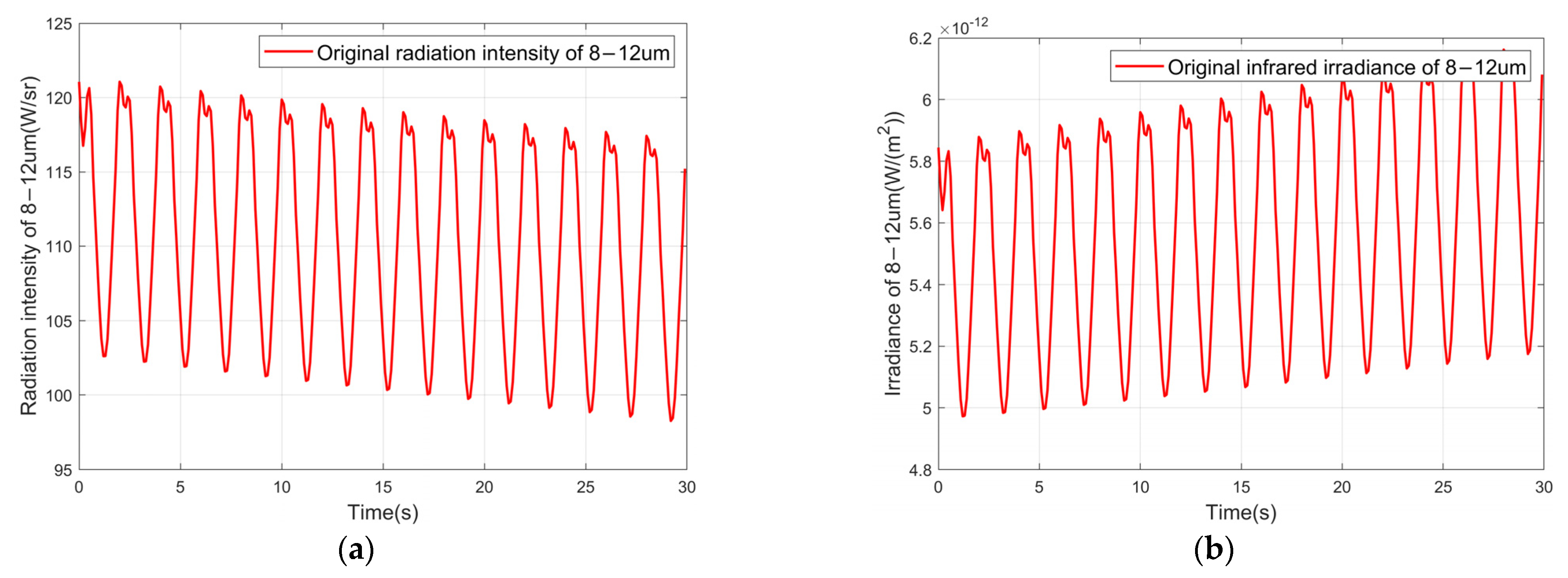
4. Simulation Parameters Setting and Construction of Infrared Simulation Signal

In this section, the simulation parameter settings and infrared simulation signal are shown. During target moving in space, micromotion occurs. This leads to a periodic oscillation of the projected area and infrared radiation of the space target in the line-of-sight (LOS) direction of the infrared detector. In this section, the target flight scenario, temperature change, and micromotion factor are considered comprehensively, and the cone-cylinder target is selected as the specific object for the simulation experiment. The parameters are shown in

Table 4. Simulation parameters.

Parameter	Value	Parameter	Value
Radius	1 m	Thickness	1 mm
Height-1	1 m	Visible absorptivity	0.45
Height-2	1 m	Emissivity	0.8
Coning rate	π rad/s	Density	2700 kg/m3
Spinning rate	4π rad/s	Specific capacity	904 J/(kg·K)
Flight environment	sunlight	Initial temperature	300 K
Frame rate	10 Hz	Observation bands	8–12 μm/6–7 μm
Observation duration	30 s	Distance	[4550.92 km, 4352.92 km]

below.

This paper [24] describes the simulation steps of the infrared radiation intensity signal of the space target. Based on the model in this article, Figure 5 shows the infrared radiation intensity signal and infrared irradiance signal of 8–12 $\mathsf{\mu }\mathrm{m}$. The waveforms of the infrared radiation intensity signal and infrared irradiance signal of 6–7 $\mathsf{\mu }\mathrm{m}$ are similar to those of 8–12 $\mathsf{\mu }\mathrm{m}$. The irradiance signal received by the infrared detector shows an upward trend in the observation duration because of the shorter distance between the target and the infrared detector. The energy oscillation shows that the target shows a flicker in the infrared image.

Prior to denoising and extracting features of the target, the signal of the target is extracted from the multi-frame infrared image. However, due to the existence of the dispersion effect of the detector, the energy of target imaging will be dispersed to adjacent pixels. Figure 6 illustrates the schematic diagram of target imaging with different diffusion radii. In addition, the effective photosensitive area of the infrared focal plane pixel is less than the actual area of the pixel, and the corresponding filling factor is less than 1 [33]. The image point of the moving target spans multiple pixels, and the total energy of the target on the image plane fluctuates. Moreover, the spatial distribution of response in a pixel is inconsistent. These factors will lead to errors in the calibration process of the detector and extracting signal. In the following, ${\mathrm{E}}_{\mathrm{cal}}$ represents the amount of error introduced by these factors.

Furthermore, considering the influence of detector noise, the irradiance model extracted from the multi-frame infrared image is as follows [34]:

$${\mathrm{E}}_{\mathrm{sn}}=\left({1+\mathrm{E}}_{\mathrm{cal}}{+\mathrm{E}}_{\mathrm{white}}\right)·\left({\mathrm{E}}_{\mathrm{s}}{+\mathrm{E}}_{\mathrm{nei}}\right)=\left({1+\mathrm{E}}_{\mathrm{com}}\right)·\left({\mathrm{E}}_{\mathrm{s}}{+\mathrm{E}}_{\mathrm{nei}}\right)$$

(35)

where ${\mathrm{E}}_{\mathrm{sn}}$ is the noisy irradiance signal, ${\mathrm{E}}_{\mathrm{s}}$ is the irradiance signal of the target, the term ${\mathrm{E}}_{\mathrm{cal}}$ is the calibration error, the term ${\mathrm{E}}_{\mathrm{white}}$ is composed of electronics and photon noise, and the latter is caused by random fluctuations in the incident flux of photons on the detector. To simplify the following contents, it is assumed that the influence of parameter ${\mathrm{E}}_{\mathrm{com}}$ on the signal is equivalent to that of these above two parameters. The term ${\mathrm{E}}_{\mathrm{nei}}$ is the NEI (noise equivalent irradiance) which means the amplitude value of irradiance signal at the entrance pupil of detector which generates a signal-to-noise ratio of 1.

For extracting the emissivity-area product, it is necessary to calculate the radiation intensity of the target according to the irradiance signal in the LOS direction on the premise of knowing the distance information. The model is as follows:

$${\mathrm{I}}_{\mathrm{s}}{=\mathrm{E}}_{\mathrm{sn}}·{\mathrm{R}}^2=\left({1+\mathrm{E}}_{\mathrm{com}}\right)\times \left({\mathrm{E}}_{\mathrm{s}}{+\mathrm{E}}_{\mathrm{nei}}\right)·{\mathrm{R}}^2$$

(36)

where ${\mathrm{I}}_{\mathrm{s}}$ is the noisy radiation intensity, $\mathrm{R}$ is the distance. Based on the above, to analyze the denoising performance of the DA-VMD algorithm, the infrared radiation intensity of 8–12 $\mathsf{\mu }\mathrm{m}$ is taken as an example. The distance measurement error is set as 100 km, the maximum value of the parameter ${\mathrm{E}}_{\mathrm{com}}$ is 2.2% and at sampling time it is randomly drawn from the uniform distribution of −0.022 to 0.022. The NEI is set to ${60\times 10}^{-14}\mathrm{W}·{\mathrm{m}}^{-2}$. Figure 7 presents the noisy radiation intensity signal extracted from multiple infrared images. It can be seen that the signal is considerably disturbed by noise and shows strong fluctuation, which causes a serious effect of feature extraction.

5. Denoising and Feature Extraction of Simulation Signal

5.1. Denoising Result and Performance Comparison with Other Methods

To suppress the amplitude of noise and improve the accuracy of feature extraction, the DA-VMD is applied to denoise and then DBT is used to extract the features of the target. In this section, we will introduce the DA-VMD is how to suppress the noise and the denoising performance comparison with other methods. Firstly, two important parameters $\mathrm{K}$ and $\mathsf{\alpha }$ of DA-VMD are optimized, the entire range of $\mathrm{K}$ and $\mathsf{\alpha }$ is set from 5 to 10 and 1500 to 8000, respectively; the number of search agents and the maximum number of iterations is 20,20, respectively. The embedding dimension of the state space vectors of the fitness function is $\mathrm{L}/2$, where L is the length of the input noisy infrared signal. Figure 8 illustrates the convergence curve of the fitness value changing with the iterations. It can be seen that the minimum fitness 0.0206 appeared in the fourteenth iteration and the corresponding parameter combination $[\mathrm{K},\mathsf{\alpha }]$ is $[10,2016]$.

Then the infrared noisy radiation signal is decomposed by VMD with the above optimal parameters to obtain 10 BLIMFs from low frequency to high frequency. The decomposed results are shown in Figure 9. The figure illustrates the time domain waveform and spectrum of 10 BLIMF components after denoising. Because of the band-limited characteristics of VMD, the BLIMFs are obtained concurrently and the frequencies of BLIMFs do not overlap. The IMFs with low-frequency oscillations are the effective modes while the high-frequency signal may be the noise. Moreover, it can be seen that the second IMF is the periodic component whose period is equal to that of coning. This provides a new idea to extract the micromotion period from noisy radiation signals.

After the decomposition ends, the effective IMFs need to be collected to reconstruct the infrared radiation signal. Calculate PCC value between each BLIMF and the original noisy signal by Equation (23). Figure 10 illustrates the result. The maximum slope of PCC appears at the second BLIMF. It is certain that the first two BLIMFs are effective and used to reconstruct the denoising signal. The reconstructed signal is shown in Figure 10 and named “DA-VMD with PCC”. It is apparent that the overall trend of the reconstructed signal is almost consistent with the noiseless signal—the noise is almost eliminated and the periodic trend is obvious. To evaluate the performance of denoising, three qua-ntitative evaluation indicators are introduced which are the signal-to-noise ratio (SNR), root-mean-square error (RMSE), and normalized correlation coefficient (NCC). The indicators are calculated as follows:

$$\mathrm{SNR}=\frac{\mathrm{mean}\left(\mathrm{x}\right(\mathrm{i}\left)\right)}{\mathrm{std}(\mathrm{f}\left(\mathrm{i}\right)-\mathrm{x}\left(\mathrm{i}\right))}$$

(37)

$$\mathrm{RMSE}=\sqrt{\frac{{{\displaystyle \sum }}_{\mathrm{i}=1}^{\mathrm{N}}{(\mathrm{f}\left(\mathrm{i}\right)-\mathrm{x}\left(\mathrm{i}\right))}^2}{\mathrm{N}}}$$

(38)

$$\mathrm{NCC}=\frac{{{\displaystyle \sum }}_{\mathrm{i}=1}^{\mathrm{N}}\left(\mathrm{f}\right(\mathrm{i}\left)\right)\left(\mathrm{x}\right(\mathrm{i}\left)\right)}{\sqrt{{{\displaystyle \sum }}_{\mathrm{i}=1}^{\mathrm{N}}{\left(\mathrm{f}\right(\mathrm{i}\left)\right)}^2·{{\displaystyle \sum }}_{\mathrm{i}=1}^{\mathrm{N}}{\left(\mathrm{x}\right(\mathrm{i}\left)\right)}^2}}$$

(39)

where $\mathrm{N}$ is the signal points, $\mathrm{x}\left(\mathrm{i}\right)$ is the noiseless signal, and $\mathrm{f}\left(\mathrm{i}\right)$ is the denoising signal.

To evaluate the effectiveness of PCC as the IMFs selection criterion, a comparison between different criteria is carried out, including the continuous mean square error (CMSE) [35] and mutual information entropy (MIE) [36], and PCC. Figure 11 shows the infrared denoisingcurves corresponding to each criterion and

Table 5. Performance of different selection criteria of effective IMFs at NEI = 60 × 10⁻¹⁴ W·m⁻².

Indicators	DA-VMD with PCC	DA-VMD with MIE	DA-VMD with CMSE
SNR	32.63	18.55	17.18
RMSE	3.48	6.01	6.48
NCC	0.91	0.78	0.76

shows the noise reduction performance index of three criteria. The SNR, RMSE, and NCC after denoising by the proposed algorithm are 32.63, 3.48, and 0.91, respectively. The indexes are superior to results of other criteria, indicating the effectiveness of PCC as the selection criterion.

In this section, we evaluate the denoising performance of the proposed method with different NEIs compared with other four methods, which are as follows: Method 1: wavelet shrinkage (Wavelet-db4); Method 2: Empirical mode decomposition (EMD); Method 3: Adaptive singular value decomposition (ASVD) [37]; Method 4: Complete ensemble empirical mode decomposition with adaptive noise (CEEMDAN). The corresponding relationship between SNR, RMSE of infrared radiation intensity signal, and NEI is shown in

Table 6. The corresponding relationship between SNR, RMSE of radiation intensity, and NEI.

NEI (W·m−2)	SNR	RMSE
120 × 10−14	4.69	24.80
80 × 10−14	6.75	16.39
60 × 10−14	9.25	11.92
40 × 10−14	13.33	9.01
30 × 10−14	17.11	6.44
20 × 10−14	22.42	4.98

. When the range of NEIs is from ${120\times 10}^{-14}\mathrm{W}·{\mathrm{m}}^{-2}$ to ${20\times 10}^{-14}\mathrm{W}·{\mathrm{m}}^{-2}$, the SNR varies from 4.69 to 22.42, and the value of RMSE decreases from 24.80 to 4.97. Figure 12 illustrates the results of different denoising methods with the NEI =${60\times 10}^{-14}\mathrm{W}·{\mathrm{m}}^{-2}$. After processing by DA-VMD, the SNR of the signal increases from 9.25 to 32.63, RMSE decreases from 11.92 to 3.48, and the NCC achieves 0.91. The denoising performance obtained by the EMD method is the worst; it has a poor recovery effect on the amplitude of the generated signal waveform, and many extreme points of the curve deviate from the original signal. The denoising signal obtained by the CEEMDAN algorithm has similar problems, in which the degree of the problem is less than that of EMD. Although Wavelet-db4 and ASVD achieve similar values in performance indexes, the amplitude of the local signal is lost in the Wavelet-db4 results, and there are many sawteeth in the ASVD result curve. The shortcomings affect the performance of these algorithms, and the performance is worse than that of the DA-VMD algorithm.

To further substantiate the above, the denoising results by these methods with NEI varying 120 × 10⁻¹⁴ W·m⁻² to 20 × 10⁻¹⁴ W·m⁻² are displayed in Figure 13. Regardless of the noise level, the DA-VMD can obtain the best denoising performance. Even in the worst case with the maximum NEI, the result of DA-VMD still guaranteed a high SNR up to 13.93. The performance comparisons in terms of RMSE and NCC at different NEI revealed that VMD-DA can achieve the minimum error in reconstructing signal. Therefore, it is concluded that the DA-VMD shows more potential denoising performance compared with the other four methods.

5.2. Feature Extraction Based on DA-VMD-DBT

It can be seen from the above that DA-VMD shows excellent performance in denoising. To test the improvement in the accuracy of the feature extraction, add different NEIs to the two infrared bands so that the SNR of the radiation intensity signal of the two bands is as close as possible. The signals of the two bands are denoised, respectively, the temperature value is calculated by using the DBT. Then, the emissivity-area product can be further obtained. For evaluating the accuracy of the features, seven statistical indexes are used: Mean value of temperature error (MV-TE), standard deviation of temperature error (SD-TE), temperature RMSE (RMSE-T), mean value of emissivity-area product error (MV-EAPE), standard deviation of emissivity-area product error (SD-EAPE), emissivity-area product RMSE (RMSE-EAP) and NCC of emissivity-area product (NCC-EAP). The NCC can characterize the similarity between the sequences of extracted features and the sequences of real feature of the target, in order to better discover the law of feature change of the target. The closer the NCC value is to 1, the more the sequence of extracted feature is similar to the sequence of real feature of the target. Also, the results of DBT, ASVD-DBT, Wd-DBT, CEEMDAN-DBT, EMD-DBT are used to compared, as shown in

Table 7. The results of evaluation indexes of the feature extraction of simulated radiation signal (8–12/6–7 μm).

Infrared Band	NEI (W∗m−2)	SNR		MV-TE (%)	SD-TE (%)	RMSE-T	MV-EAP (%)	SD-EAP (%)	RMSE-EAP	NCC-EAP
8–12 μm 6–7 μm	120∗10−14 200∗10−15	4.69 4.56	DBT	10.05	8.35	44.58	88.36	117.35	3.77	−0.04
			ASVD-DBT	3.37	2.59	12.81	25.14	21.32	0.90	0.14
			Wd-DBT	3.93	2.98	14.74	31.51	28.57	1.17	0.12
			CEEMDAN-DBT	3.35	3.41	13.52	30.22	25.00	1.08	0.05
			EMD-DBT	3.94	3.07	14.94	31.58	27.43	1.14	0.13
			DA-VMD-DBT	3.19	2.22	13.14	27.07	21.64	0.85	0.15
8–12 μm 6–7 μm	80∗10−14 130∗10−15	6.75 6.49	DBT	6.96	5.07	25.96	52.07	50.02	1.86	0.065
			ASVD-DBT	2.80	2.32	10.89	19.26	17. 80	0.72	0.19
			Wd-DBT	2.64	1.77	9.51	18.56	12.97	0.62	0.28
			CEEMDAN-DBT	2.63	1.93	9.76	19.19	15.08	0.67	0.21
			EMD-DBT	3.61	2.60	11.31	25.82	21.57	0.92	0.19
			DA-VMD-DBT	1.89	1.53	9.73	15.74	13.59	0.77	0.25
8–12 μm 6–7 μm	60∗10−14 90∗10−15	9.25 10.02	DBT	5.14	3.64	18.22	35.34	29.01	1.24	0.16
			ASVD-DBT	2.21	1.60	8.16	16.99	13.25	0.60	0.34
			Wd-DBT	1.92	1.38	7.09	16.30	11.22	0.54	0.39
			CEEMDAN-DBT	1.99	1.63	7.70	15.17	13.68	0.57	0.47
			EMD-DBT	2.36	1.93	9.11	18.53	14.99	0.65	0.37
			DA-VMD-DBT	1.34	0.87	5.57	11.37	7.18	0.41	0.52
8–12 μm 6–7 μm	40∗10−14 65∗10−15	13.33 14.62	DBT	3.22	2.52	11.56	23.16	21.68	0.88	0.19
			ASVD-DBT	1.78	1.42	6.81	12.76	10.49	0.46	0.39
			Wd-DBT	1.01	0.79	3.85	8.93	6.99	0.31	0.45
			CEEMDAN-DBT	1.02	0.75	3.79	8.55	6.32	0.30	0.52
			EMD-DBT	1.84	1.32	6.79	12.95	9.35	0.44	0.48
			DA-VMD-DBT	0.83	0.65	4.34	8.37	5.44	0.38	0.63
8–12 μm 6–7 μm	30∗10−14 45∗10−15	17.11 17.88	DBT	2.45	1.89	9.01	18.18	15.31	0.64	0.36
			ASVD-DBT	0.96	0.67	4.23	8.87	5.97	0.33	0.64
			Wd-DBT	0.90	0.67	3.3	8.92	6.54	0.30	0.50
			CEEMDAN-DBT	1.17	0.79	4.23	9.38	7.27	0.33	0.64
			EMD-DBT	1.72	1.33	5.53	11.05	9.95	0.42	0.75
			DA-VMD-DBT	0.73	0.48	3.01	8.28	4.39	0.28	0.77
8–12 μm 6–7 μm	20∗10−14 30∗10−15	22.42 21.67	DBT	1.71	1.34	6.39	13.38	10.43	0.47	0.43
			ASVD-DBT	0.97	0.65	3.49	10.60	5.91	0.33	0.67
			Wd-DBT	0.79	0.53	2.86	8.30	5.09	0.27	0.70
			CEEMDAN-DBT	0.96	0.60	3.38	10.16	5.61	0.32	0.67
			EMD-DBT	1.30	0.91	4.77	10.71	7.90	0.38	0.76
			DA-VMD-DBT	0.64	0.36	2.16	7.64	3.48	0.24	0.79

.

It can be seen that the performance of the proposed algorithm outperforms other algorithms in general. The accuracies of temperature and emissivity-area product using the proposed algorithm are improved by about 2.8 times and 2.5 times on average than those of DBT respectively, and the similarity of the sequence of emissivity area product is also improved. However, when the SNR is about 4.6, the MV-EAPE is about 27.07% even using DA-VMD-DBT, and when the SNR is about 22, the MV-EAPE is close to 7.63%, which is also quite high compared with 0.64% of the MV-TE. This is because to obtain the emissivity-area product, the temperature and the measured distance need to be used, and the coupling error of the two information also affects the accuracy of the emissivity-area product in addition to NEI. Hence, it can be concluded that the accuracy of the emissivity-area product is more vulnerable to external parameters compared with temperature. To improve the feature accuracy of the emissivity-area product, it is necessary to reduce the errors of the above three factors.

To intuitively understand the distribution of error data of 8–12/6–7 $\mathsf{\mu }\mathrm{m}$, a box diagram is displayed, as shown in Figure 14. The diagram shows the distribution of temperature relative error before and after denoising, and also shows the distribution of emissivity-area product relative error before and after denoising. The maximum, minimum, median, two quartiles, and outliers of the error can be intuitively understood. Comparing the results before and after denoising, it is found that the temperature error after denoising is effectively improved, and the error of the emissivity-area product is reduced most significantly. Moreover, after denoising, the number of error outliers and the degree of the anomaly are reduced.

To comprehensively evaluate the effect of the proposed algorithm in other band combinations,

Table 8. The results of evaluation indexes of the feature extraction of simulated radiation signal (8–12/3–5 μm).

Infrared Band	NEI (W∗m−2)	SNR		MV-TE (%)	SD-TE (%)	RMSE-T	MV-EAP (%)	SD-EAP (%)	RMSE-EAP	NCC-EAP
8–12 μm 3–5 μm	120∗10−14 200∗10−15	4.69 1.67	DBT	10.10	7.25	37.17	96.38	170.67	6.42	0.055
			ASVD-DBT	4.94	3.37	16.85	24.42	24.05	0.95	0.21
			Wd-DBT	4.62	2.87	16.29	18.30	13.88	0.63	0.24
			CEEMDAN-DBT	5.11	3.44	17.91	24.21	19.16	0.84	0.21
			EMD-DBT	4.32	3.17	14.17	16.76	10.98	0.54	0.30
			DA-VMD-DBT	4.19	2.30	14.29	20.08	15.78	0.69	0.28
8–12 μm 3–5 μm	80∗10−14 130∗10−15	6.75 2.43	DBT	7.44	6.16	28.86	46.29	71.62	2.40	0.076
			ASVD-DBT	4.32	3.37	17.18	19.74	14.86	0.68	0.42
			Wd-DBT	3.52	2.65	13.18	14.83	10.13	0.49	0.39
			CEEMDAN-DBT	4.15	2.46	14.41	16.68	11.42	0.56	0.46
			EMD-DBT	3.81	2.79	13.09	10.35	8.41	0.47	0.49
			DA-VMD-DBT	3.41	2.31	12.32	16.78	11.59	0.68	0.51
8–12 μm 3–5 μm	60∗10−14 90∗10−15	9.25 3.50	DBT	5.32	3.93	19.77	29.14	38.83	1.34	0.34
			ASVD-DBT	3.41	2.31	12.34	14.59	10.44	0.50	0.47
			Wd-DBT	2.92	1.84	10.33	11.79	7.68	0.38	0.57
			CEEMDAN-DBT	3.45	1.76	11.47	13.38	9.05	0.43	0.60
			EMD-DBT	3.01	1.78	10.46	13.13	7.72	0.43	0.62
			DA-VMD-DBT	2.96	1.74	10.28	11.01	6.88	0.36	0.65
8–12 μm 3–5 μm	40∗10−14 65∗10−15	13.33 4.54	DBT	4.16	2.85	15.07	20.17	16.71	0.73	0.38
			ASVD-DBT	3.22	2.17	11.62	13.48	9.94	0.46	0.52
			Wd-DBT	3.02	1.68	9.79	11.25	6.07	0.33	0.58
			CEEMDAN-DBT	2.49	1.76	9.14	10.44	6.72	0.31	0.68
			EMD-DBT	3.08	1.63	10.42	10.69	7.35	0.38	0.66
			DA-VMD-DBT	2.97	1.53	9.99	9.89	5.59	0.31	0.74
8–12 μm 3–5 μm	30∗10−14 45∗10−15	17.11 6.15	DBT	3.52	2.32	12.61	15.50	10.70	0.52	0.46
			ASVD-DBT	2.71	1.56	9.35	9.01	6.16	0.29	0.73
			Wd-DBT	3.07	1.22	9.89	10.04	5.03	0.31	0.72
			CEEMDAN-DBT	2.87	1.63	9.86	8.93	6.03	0.29	0.75
			EMD-DBT	3.08	1.57	10.34	10.01	6.85	0.34	0.71
			DA-VMD-DBT	2.75	1.29	9.07	8.76	5.51	0.29	0.80
8–12 μm 3–5 μm	20∗10−14 30∗10−15	22.42 9.88	DBT	3.00	1.92	10.65	11.17	7.48	0.37	0.61
			ASVD-DBT	2.91	1.05	9.25	8.64	5.03	0.27	0.88
			Wd-DBT	3.02	1.14	9.68	8.89	5.30	0.28	0.76
			CEEMDAN-DBT	2.90	1.22	9.42	8.45	4.32	0.28	0.81
			EMD-DBT	2.96	1.44	10.23	9.68	6.23	0.31	0.84
			DA-VMD-DBT	2.76	1.20	9.00	8.88	4.68	0.27	0.88

shows the accuracy of feature extraction of utilizing 8–12/3–5 $\mathsf{\mu }\mathrm{m}$. As shown in the table, keep the NEI unchanging, the error of feature extraction of utilizing 8–12/3–5 $\mathsf{\mu }\mathrm{m}$ is higher than that of utilizing 8–12/6–7 $\mathsf{\mu }\mathrm{m}$ in general. For example, when the NEIs are ${20\ast 10}^{-14}$ W∗m⁻² and ${30\ast 10}^{-15}$ W∗m⁻² respectively, for the proposed algorithm, the accuracies of the temperature and emissivity-area product are 2.7%, 9% of utilizing 8–12/3–5 $\mathsf{\mu }\mathrm{m}$, higher than 0.64% and 7.64% of utilizing 8–12/6–7 $\mathsf{\mu }\mathrm{m}$, respectively. Also, it can be predicted that if continuing to enhance the SNR, the accuracies of feature extraction of 8–12/3–5 $\mathsf{\mu }\mathrm{m}$ cannot be further improved, which also proves the superiority of 8–12/6–7 $\mathsf{\mu }\mathrm{m}$ in feature extraction.

6. Experimental Verification of the Proposed Algorithm

6.1. Introduction of Experiment

To verify the effectiveness of the proposed method in the denoising and extracting feature, a semi-physical simulation platform for space infrared dim target detection and recognition is designed and built to obtain the temperature value, micromotion info-rmation, and infrared radiation signal. Figure 15 illustrates a physical diagram of the platform and two infrared detectors. Two motors are used to simulate the micromotion of the space target. The position of each motor in the overall system is shown, in which the bottom motor controls the coning rotation movement of the target and the top motor controls the spinning movement. To prevent the power lines of the two motors from winding during rotation, which makes it impossible to carry out micromotion simulation, a conductive slip ring is used to avoid winding in the design process. The overall heating module is composed of a heating sheet and a temperature controller. It can be used to simulate the temperature change process of the target. The range of heating temperature is 30 °C to 100 °C. A thermometer is used to measure the temperature of the target, and its resolution is 0.1 °C. The parameters of the two infrared detectors are shown in

Table 9. Parameters setting of the two infrared detectors.

Parameter Name	Infrared Detector 1	Infrared Detector 2
Spectral range (μm)	8–11.7	3–5
Resolution (pixel)	320 × 256	640 × 512
Pixel size (μm)	30	15
Focal length (mm)	100	200
Optical aperture (cm)	5	5

.

In this experiment, the ball-base-cone is taken as an example. The height of the cone is 20 cm, the radius of the hemisphere is 5 cm, its surface material is a black film, and the emissivity is 0.85. During the experiment, the temperature of the target was maintained at 40 °C the coning period was 1.5 s and the spin period was 0.9 s. The distance between the target and detector was 10.9 $\mathrm{m}$. The images after reshaping in the two infrared bands of the target are shown in Figure 16.

6.2. Denoising and Extracting Features of Experiment Data

In the test experiment, because the frame rates of the two detectors are different, the infrared data points in the two bands cannot correspond. Therefore, it is necessary to interpolate, match and align the data points at the same time. After processing, the radiation intensity signal sequence of the target is extracted from the images of two infrared bands, as shown in Figure 17. The length of collected data is 380 data points. It seems that the signal is regular and has almost no noise interference. This is due to the limited distance in the laboratory environment. The infrared radiation intensity received by the detector is much greater than the NEI of the detector, and the image of the target is a typical area target rather than a dim point target. Therefore, by adding different intensities of the noise of the radiation intensity of the target in the laboratory, the testing data can be obtained for verifying the denoising and extracting features of the proposed algorithm.

To verify the denoising effectiveness of the DA-VMD algorithm on the experimental data, different intensities of noise are added to the experimental data. Taking the radiation intensity of 8–11.7 $\mathsf{\mu }\mathrm{m}$ with SNR = 10 as an example, firstly, according to the mean weight FuzzDistEn, the optimal parameters of the VMD method are iteratively optimized and the combination is (K, α) = (6, 1500). Then, decompose the noisy signal using the VMD, remove the noise component, and reconstruct the effective signal. The resulting signal is shown in Figure 18. Compared to the other methods, the DA-VMD method eliminated the noise more accurately and maintained the changing trend of the original signal to the maximum extent. Moreover, when the SNR is 5, 10, 15, 20, and 25, the results of three evaluation indexes of different methods are shown in Figure 19. It can be seen that the proposed methods can effectively denoise and obtain the best denoising performance.

Table 10. The results of evaluation indexes of the feature extraction of experiment data (8–11.7/3–5 μm).

Infrared Band		SNR		MV-TE (%)	SD-TE (%)	RMSE-T	MV-EAP (%)	SD-EAP (%)	RMSE-EAP	NCC-EAP
8–11.7 μm 3–5 μm	5 5		DBT	4.38	3.11	16.80	43.34	37.27	0.0084	0.018
			ASVD-DBT	2.37	1.39	8.59	22.89	15.52	0.0040	0.084
			Wd-DBT	2.20	1.27	7.95	21.47	14.05	0.0037	0.11
			CEEMDAN-DBT	2.49	1.10	8.54	22.83	11.99	0.0037	0.13
			EMD-DBT	2.23	1.31	8.09	21.21	13.33	0.0036	0.09
			DA-VMD-DBT	1.99	1.17	7.23	19.46	13.57	0.0035	0.11
8–11.7 μm 3–5 μm	10 10		DBT	2.41	1.71	9.24	23.38	19.25	0.0045	0.10
			ASVD-DBT	2.32	0.74	7.65	20.15	6.68	0.0031	0.33
			Wd-DBT	2.27	0.82	7.57	20.27	8.35	0.0032	0.42
			CEEMDAN-DBT	2.27	0.78	7.51	19.53	7.84	0.0031	0.41
			EMD-DBT	2.38	0.83	7.89	21.20	8.66	0.0034	0.31
			DA-VMD-DBT	2.08	0.65	6.81	19.27	6.47	0.0030	0.47
8–11.7 μm 3–5 μm	15 15		DBT	2.13	1.44	8.04	19.87	14.08	0.0036	0.21
			ASVD-DBT	2.20	0.53	7.09	19.69	4.62	0.0030	0.58
			Wd-DBT	2.26	0.62	7.35	20.66	5.99	0.0032	0.50
			CEEMDAN-DBT	2.24	0.50	7.18	20.04	4.66	0.0030	0.49
			EMD-DBT	2.21	0.65	7.21	20.36	6.74	0.0032	0.53
			DA-VMD-DBT	1.99	0.44	6.38	17.67	4.00	0.0027	0.61
8–11.7 μm 3–5 μm	20 20		DBT	2.23	1.13	7.82	20.72	11.63	0.0035	0.28
			ASVD-DBT	2.23	0.42	7.12	19.36	3.63	0.0029	0.65
			Wd-DBT	2.28	0.38	7.25	20.36	4.30	0.0031	0.62
			CEEMDAN-DBT	2.23	0.48	7.01	20.04	3.01	0.0029	0.65
			EMD-DBT	2.23	0.47	7.13	20.25	4.42	0.0031	0.56
			DA-VMD-DBT	2.22	0.36	7.03	20.06	3.74	0.0030	0.74
8–11.7 μm 3–5 μm	25 25		DBT	2.17	0.97	7.42	19.86	9.66	0.0033	0.32
			ASVD-DBT	2.17	0.37	6.84	19.65	2.90	0.0029	0.77
			Wd-DBT	2.20	0.43	7.02	19.87	3.73	0.0030	0.64
			CEEMDAN-DBT	2.19	0.47	7.01	19.70	4.15	0.0029	0.62
			EMD-DBT	2.21	0.51	7.09	19.91	4.16	0.0030	0.74
			DA-VMD-DBT	2.16	0.33	6.84	19.50	3.02	0.0029	0.87

shows results of evaluation indexes of the feature extraction of the experimental data within differeret algorithms under different SNRs. From the table, when the SNR is 5, for the proposed algorithm, the average error of temperature is reduced by about 2.39%, the average error of the emissivity-area product is reduced by about 23.88%, and the standard deviation and the RMSE of the two features are reduced. However, for these agorithms, when the SNR is greater than or equal to 15, the average error of the two features rarely changes after noise reduction, the standard deviation and RMSE are decreased. This is because the main factor affecting the feature accuracy is the reflected external radiation of the target for SNR $\ge 15$ and the dispersion of error of the two features still be reduced after denoising. Also, the NCC-EAP is still increased, which the similarity of extracted emissivity-area product to real emissivity-area product is better.

7. Discussion

When the infrared detector detects and images the space target, the self-radiation of the target is coupled with the external radiation reflected by the target, which is often unable to be separated. The external radiation reflected by target is an important factor affecting the accuracy of target feature. According to Planck’s law and Kirchhoff’s law, the amount of external radiation reflected by the target entering the photosensitive surface of detectors is related not only to the property of the target itself (such as the infrared emissivity), but also to the infrared band of detector. Therefore, the reasonable infrared band combination is designed and selected to reduce the influence of external radiation on the accuracy of temperature and emissivity-area product. The selection of infrared band also needs to consider the bands of existing infrared detectors in the aerospace field.

On the basis of the selection of infrared band combination, the simulation data and measured data in the lab are processed by DA-VMD-DBT to realize denoising and feature extraction for space infrared dim target recognition. From the simulation results show that the accuracy of feature extraction has been improved after denoising, also, the feature extraction results of different band combinations are compared. For example, for the proposed algorithm in the paper, when the SNR of simulation signals of 8–12/6–7 $\mathsf{\mu }\mathrm{m}$ is about 10, the MV-TE and the MV-EAP are reduced to 1.34%, 11.37%, respectively; under the same conditions, the MV-TE and the MV-EAP of 8–12/3–5 $\mathsf{\mu }\mathrm{m}$ are reduced to 2.97%, 9.87%, respectively. It can be concluded that the accuracy of temperature of 8–12/6–7 $\mathsf{\mu }\mathrm{m}$ is superior to that of 8–12/3–5 $\mathsf{\mu }\mathrm{m}$, the accuracy of emissivity-area product of 8–12/6–7 $\mathsf{\mu }\mathrm{m}$ is almost equal to that of 8–12/3–5 $\mathsf{\mu }\mathrm{m}$. This proves the advantages of utilizing 8–12/6–7 $\mathsf{\mu }\mathrm{m}$ to extract feature. For the measured data of 8–11.7/3–5 $\mathsf{\mu }\mathrm{m}$ in the lab, when the SNR of infrared signals is less than 15, The accuracy of feature extraction obtained by the proposed algorithm is significantly improved. The simulation and experimental results show the effectiveness of DA-VMD-DBT in the field of denoising and feature extraction.

Interestingly, the period of one BLIMF decomposed by VMD is equal to the micromotion period of the target. This is because that the VMD can decompose the input signal into a series of modes, and the modes is sparsity which compact around a center pulsation, namely the frequency of the modes. It provides a potential possibility to extract the micromotion period of the target based on these BLIMFs. However, the effectiveness of the proposed algorithm has been verified, its feasibility needs to be further analyzed and investigated by a large number of simulation signals and measured signals. Furthermore, in the process of optimizing VMD parameters, a large-scale calculation limits the online operation. Further work is needed to explore to reduce consumption of time and computing resources.

8. Conclusions

To accurately extract the features of the temperature and the emissivity-area product from infrared noisy signals, a novel technique that integrates DA, VMD, and DBT is proposed in this paper. The main contributions of the paper can be listed as follows:

(1)

The selection of infrared band combination is carried out. By analyzing the accuracy of feature extraction of space targets with different emissivity and absorptivity under different band combinations, 8–12/6–7 μm is regarded as ideal selection. Using this band combination can reduce the influence of external radiation reflected by target on feature extraction.

(2)

The DA-VMD module is used for denoising signal. For the denoising, the DA and the mean weighted FuzzDistEn are used to search for the optimal combination of parameters (K, α). The VMD with the optimal parameters decomposes the infrared noisy signal to K BLIMFs, and the effective BLIMFs are selected by the PCC to reconstruct the denoising signal. The effectiveness of the module is analyzed and compared with Wavelet-db4, ASVD, EMD, and CEEMDAN by using the simulated infrared radiation intensity signal of the cone-cylinder and the measured signal of the ball-base-cone in the laboratory. The simulation and experimental results demonstrate that the DA-VMD outperforms four methods in terms of SNR, RMSE, NCC and gets better performance of denoising.

(3)

The DBT module is introduced to measure the features of the temperature and the emissivity-area product. The DA-VMD-DBT outperform other algorithms in the paper. The result can be concluded that the proposed algorithm can effectively extract the features of temperature and emissivity-area product from the infrared dim noisy signals.

References

1. Erlandson, R.E.; Taylor, J.C.; Michaelis, C.H.; Edwards, J.L.; Brown, R.C.; Swaminathan, P.K.; Kumar, C.K.; Hargis, C.B.; Goldberg, A.C.; Klatt, E.M.; et al. Development of Kill Assessment Technology for Space-Based Applications. Johns Hopkins APL Tech. Dig. 2010, 29, 289. [Google Scholar]
2. Yılmaz, Ö.; Aouf, N.; Checa, E.; Majewski, L.; Sanchez-Gestido, M. Thermal analysis of space debris for infrared-based active debris removal. Proc. Inst. Mech. Eng. Part G J. Aerosp. Eng. 2019, 233, 811–822. [Google Scholar] [CrossRef]
3. Chen, L.; Rao, P.; Chen, X. Infrared dim target detection method based on local feature contrast and energy concentration degree. Optik 2021, 248, 167651. [Google Scholar] [CrossRef]
4. Zhu, H.; Li, Y.; Hu, T. Key parameters design of an aerial target detection system on a space-based platform. Opt. Eng. 2018, 57, 023107. [Google Scholar] [CrossRef]
5. Deng, Q.; Lu, H.; Hu, M.; Zhao, B. Exo-atmospheric infrared objects classification using recurrence-plots-based convolutional neural networks. Appl. Opt. 2019, 58, 164–171. [Google Scholar] [CrossRef]
6. Liu, J.; Wu, Y.; Lu, H.; Zhao, B. Micromotion dynamics and geometrical shape parameters estimation of exo-atmospheric infrared targets. Opt. Eng. 2016, 55, 113103. [Google Scholar] [CrossRef]
7. Reddy, T.S. Noise reduction in LIDAR signal using wavelets. Int. J. Eng. Technol. 2009, 2, 21–28. [Google Scholar]
8. Yuan, R.; Lv, Y.; Song, G. Fault diagnosis of rolling bearing based on a novel adaptive high-order local projection denoising method. Complexity 2018, 2018, 3049318. [Google Scholar] [CrossRef] [Green Version]
9. Xu, X.; Luo, M.; Tan, Z.; Pei, R. Echo signal extraction method of laser radar based on improved singular value decomposition and wavelet threshold denoising. Infrared Phys. Technol. 2018, 92, 327–335. [Google Scholar] [CrossRef]
10. Huang, N.E.; Shen, Z.; Long, S.R.; Wu, M.C.; Shih, H.H.; Yen, N.; Tung, C.C.; Liu, H.H. The empirical mode decomposition and the Hilbert spectrum for nonlinear and non-stationary time series analysis. Proc. R. Soc. Lond. Ser. A Math. Phys. Eng. Sci. 1998, 454, 903–995. [Google Scholar] [CrossRef]
11. Torres, M.E.; Colominas, M.A.; Schlotthauer, G.; Flandrin, P. A complete ensemble empirical mode decomposition with adaptive noise. In Proceedings of the 2011 IEEE International Conference on Acoustics, Speech and Signal Processing (ICASSP), Prague, Czech Republic, 22–27 May 2011; pp. 4144–4147. [Google Scholar]
12. Dragomiretskiy, K.; Zosso, D. Variational mode decomposition. IEEE Trans. Signal Process. 2013, 62, 531–544. [Google Scholar] [CrossRef]
13. Ahmed, W.A.; Wu, F.; Marlia, D.; Ednofri; Zhao, Y. Mitigation of Ionospheric Scintillation Effects on GNSS Signals with VMD-MFDFA. Remote Sens. 2019, 11, 2867. [Google Scholar] [CrossRef] [Green Version]
14. Kumar, A.; Zhou, Y.; Xiang, J. Optimization of VMD using kernel-based mutual information for the extraction of weak features to detect bearing defects. Measurement 2021, 168, 108402. [Google Scholar] [CrossRef]
15. Fu, J.; Cai, F.; Guo, Y.; Liu, H.; Niu, W. An Improved VMD-Based Denoising Method for Time Domain Load Signal Combining Wavelet with Singular Spectrum Analysis. Math. Probl. Eng. 2020, 2020, 1485937. [Google Scholar] [CrossRef]
16. Li, Y.; Li, Y.; Chen, X.; Yu, J. Denoising and feature extraction algorithms using NPE combined with VMD and their applications in ship-radiated noise. Symmetry 2017, 9, 256. [Google Scholar] [CrossRef] [Green Version]
17. Zhao, Y.; Li, C.; Fu, W.; Liu, J.; Yu, T.; Chen, H. A modified variational mode decomposition method based on envelope nesting and multi-criteria evaluation. J. Sound Vib. 2020, 468, 115099. [Google Scholar] [CrossRef]
18. Liu, Y.; Yang, G.; Li, M.; Yin, H. Variational mode decomposition denoising combined the detrended fluctuation analysis. Signal Process. 2016, 125, 349–364. [Google Scholar] [CrossRef]
19. Li, Y.; Chen, X.; Yu, J.; Yang, X.; Yang, H. The data-driven optimization method and its application in feature extraction of ship-radiated noise with sample entropy. Energies 2019, 12, 359. [Google Scholar] [CrossRef] [Green Version]
20. Lian, J.; Liu, Z.; Wang, H.; Dong, X. Adaptive variational mode decomposition method for signal processing based on mode characteristic. Mech. Syst. Signal Process. 2018, 107, 53–77. [Google Scholar] [CrossRef]
21. Li, C.; Peng, T.; Zhu, Y. A Novel Approach for Acoustic Signal Processing of a Drum Shearer Based on Improved Variational Mode Decomposition and Cluster Analysis. Sensors 2020, 20, 2949. [Google Scholar] [CrossRef]
22. Mirjalili, S. Dragonfly algorithm: A new meta-heuristic optimization technique for solving single-objective, discrete, and multi-objective problems. Neural Comput. Appl. 2016, 27, 1053–1073. [Google Scholar] [CrossRef]
23. Kumar, S.; Rajamani, D.; Balsubramanian, E. Experimental Investigations and Multi-Objective Optimization of Selective Inhibition Sintering Process Using the Dragonfly Algorithm. Applications of Artificial Intelligence in Additive Manufacturing. In Advances in Computational Intelligence and Robotics; IGI Global: Hershey, PA, USA, 2022; pp. 96–113. [Google Scholar]
24. Zhang, H.; Rao, P.; Xia, H.; Weng, D.; Chen, X.; Li, Y. Modeling and analysis of infrared radiation dynamic characteristics for space micromotion target recognition. Infrared Phys. Technol. 2021, 116, 103795. [Google Scholar] [CrossRef]
25. Araújo, A.; Martins, N. Monte Carlo simulations of ambient temperature uncertainty determined by dual-band pyrometry. Meas. Sci. Technol. 2015, 26, 085016. [Google Scholar] [CrossRef]
26. Araújo, A.; Silvano, S.; Martins, N. Monte Carlo uncertainty simulation of surface emissivity at ambient temperature obtained by dual spectral infrared radiometry. Infrared Phys. Technol. 2014, 67, 131–137. [Google Scholar] [CrossRef]
27. Araújo, A. Analysis of multi-band pyrometry for emissivity and temperature measurements of gray surfaces at ambient temperature. Infrared Phys. Technol. 2016, 76, 365–374. [Google Scholar] [CrossRef]
28. Duan, J.; Wang, P.; Ma, W.; Tian, X.; Fang, S.; Cheng, Y.; Chang, Y.; Liu, H. Short-term wind power forecasting using the hybrid model of improved variational mode decomposition and Correntropy Long Short-term memory neural network. Energy 2021, 214, 118980. [Google Scholar] [CrossRef]
29. Zhou, Q.; Zhang, J.; Zhou, T.; Qiu, Y.; Jia, H.; Lin, J. A parameter-adaptive variational mode decomposition approach based on weighted fuzzy-distribution entropy for noise source separation. Meas. Sci. Technol. 2020, 31, 125004. [Google Scholar] [CrossRef]
30. Li, P.; Liu, C.; Li, K.; Zheng, D.; Liu, C.; Hou, Y. Assessing the complexity of short-term heartbeat interval series by distribution entropy. Med. Biol. Eng. Comput. 2015, 53, 77–87. [Google Scholar] [CrossRef]
31. Chang, Y.; Bao, G.; Cheng, S.; He, T.; Yang, Q. Improved VMD-KFCM algorithm for the fault diagnosis of rolling bearing vibration signals. IET Signal Process. 2021, 15, 238–250. [Google Scholar] [CrossRef]
32. Zhou, S. Introduction to Advanced Infrared Photoelectricity Engineering, 1st ed.; Science Press: Beijing, China, 2016; pp. 23–24. [Google Scholar]
33. Wang, Y. On-orbit Radiometric Calibration Method for Gaze Camera with Large Planar Array. Ph.D. Thesis, Shanghai Institute of Technical Physics, Chinese Academy of Sciences, Shanghai, China, 2019. [Google Scholar]
34. Resch, C. Exo-atmospheric discrimination of thrust termination debris and missile segments. Johns Hopkins APL Tech. Dig. 1998, 19, 315. [Google Scholar]
35. Lu, Q.; Pang, L.; Huang, H.; Shen, C.; Cao, H.; Shi, Y.; Liu, J. High-G calibration denoising method for high-G MEMS accelerometer based on EMD and wavelet threshold. Micromachines 2019, 10, 134. [Google Scholar] [CrossRef] [PubMed] [Green Version]
36. Lei, Z.; Su, W.; Hu, Q. Multimode decomposition and wavelet threshold denoising of mold level based on mutual information entropy. Entropy 2019, 21, 202. [Google Scholar] [CrossRef] [PubMed] [Green Version]
37. Ashtiani, M.B.; Shahrtash, S.M. Partial discharge de-noising employing adaptive singular value decomposition. IEEE Trans. Dielectr. Electr. Insul. 2014, 21, 775–782. [Google Scholar] [CrossRef]
Figure 1. Radiation diagram from the space target to the infrared detector.
Machines 10 00168 g001
Figure 2. Flowchart of the proposed method.
Machines 10 00168 g002
Figure 3. Temperature and emissivity-area product error percentage and RMSE (ϵ = 0.5) (a) temperature error percentage (b) temperature RMSE (c) emissivity-area product error percentage (d) emissivity-area product RMSE.
Machines 10 00168 g003
Figure 4. The ratios of self-radiation to the total radiation. (a) the ratios in different infrared bands(absorptivity = 0.9, emissivity); (b) the ratios within 3–5 μm.
Machines 10 00168 g004
Figure 5. The infrared radiation intensity signal and infrared irradiance signal of 8–12 μm. (a) Infrared radiation intensity; (b) infrared irradiance signal.
Machines 10 00168 g005
Figure 6. Dispersion effect distribution diagram of point target (a) dispersion radius of 1.5 pixels; (b) dispersion radius of 2.5 pixels.
Machines 10 00168 g006
Figure 7. The noisy radiation intensity signal.
Machines 10 00168 g007
Figure 8. DA convergence curve for VMD parameter optimization.
Machines 10 00168 g008
Figure 9. The BLIMFs waveform and frequency spectrum waveform of each BLIMF after decom-position of DA-VMD. (a) Time domain waveform of BLIMFs; (b) frequency spectrum waveform of each BLIMF.
Machines 10 00168 g009
Figure 10. PCC value between BLIMFs and the noisy radiation signal.
Machines 10 00168 g010
Figure 11. Denoising signal of different selection criteria of effective IMFs.
Machines 10 00168 g011
Figure 12. Denoising signal of different denoising methods with the NEI = 60 × 10−14 W·m−2.
Machines 10 00168 g012
Figure 13. Denoising performance with different NEIs of the noisy radiation intensity signal of the cone-cylinder; (a) SNR; (b) RMSE; (c) NCC.
Machines 10 00168 g013
Figure 14. Box diagram of error of features by using DBT and DA-VMD-DBT. (a) Temperature error of DBT; (b) temperature error of DA-VMD-DBT; (c) emissivity-area product error of DBT; (d) emissivity-area product error of DA-VMD-DBT.
Machines 10 00168 g014
Figure 15. Physical diagram of the platform and two infrared detectors. (a) the physical diagram of the semi-physical simulation platform; (b) the infrared detector 1; (c) the infrared detector 2.
Machines 10 00168 g015
Figure 16. Infrared images after reshaping; (a) 8–11.7 μm; (b) 3–5 μm.
Machines 10 00168 g016
Figure 17. Radiation intensity extracting from multi-frame images; (a) 8–11.7 μm; (b) 3–5 μm.
Machines 10 00168 g017
Figure 18. Denoising signal of different denoising methods with SNR = 10 (8–11.7 μm).
Machines 10 00168 g018
Figure 19. Denoising signal of different denoising methods with SNR = 10 (8–11.7 μm). (a) SNR; (b) RMSE; (c) NCC.
Machines 10 00168 g019