
Study on Corrective Abrasive Finishing for Workpiece Surface by Using Magnetic Abrasive Finishing Processes


Abstract
:1. Introduction
2. Processing Principle
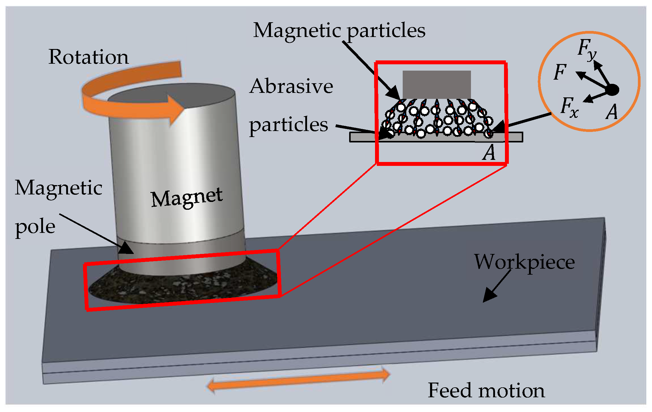
2.1. Processing Principle of Magnetic Abrasive Finishing
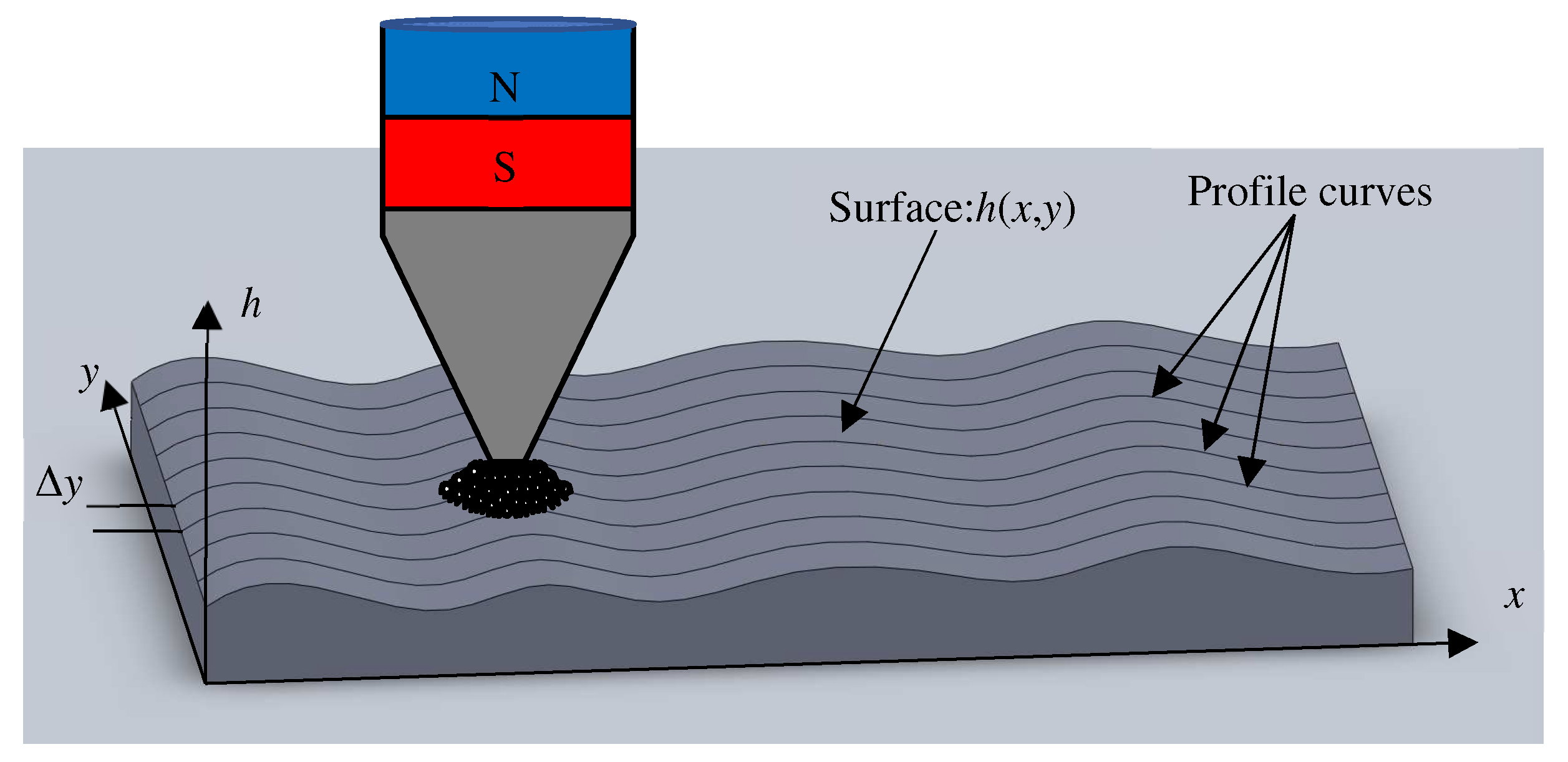
2.2. Processing Principle of Corrective Magnetic Abrasive Finishing
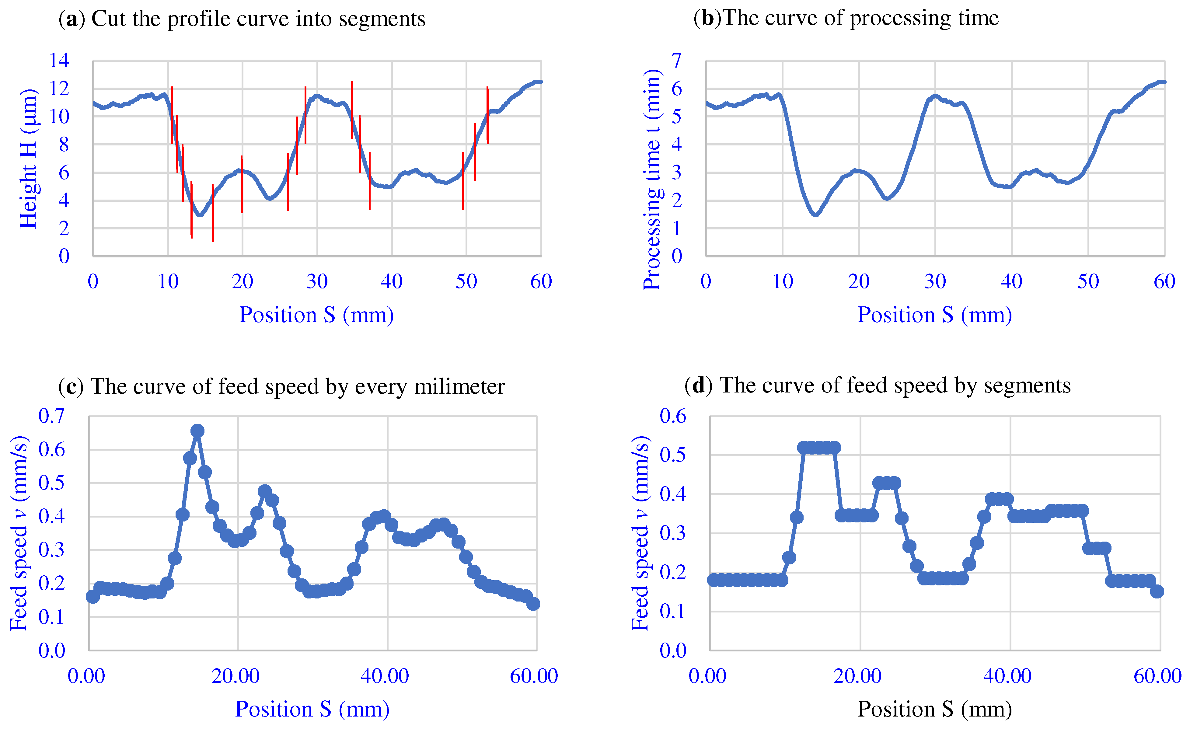
2.3. Calculation of Feed Speed Array
3. Experimental Stage
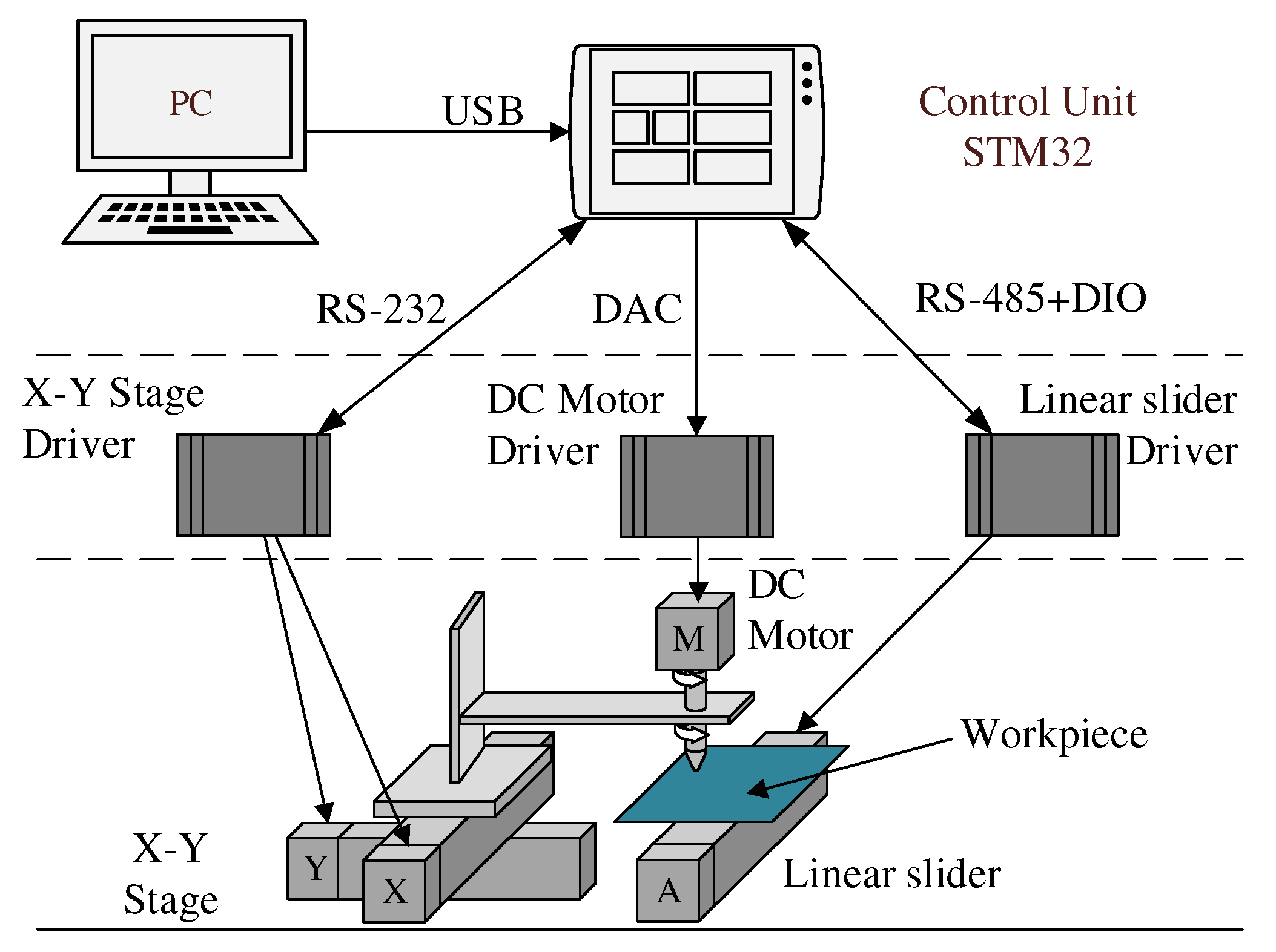
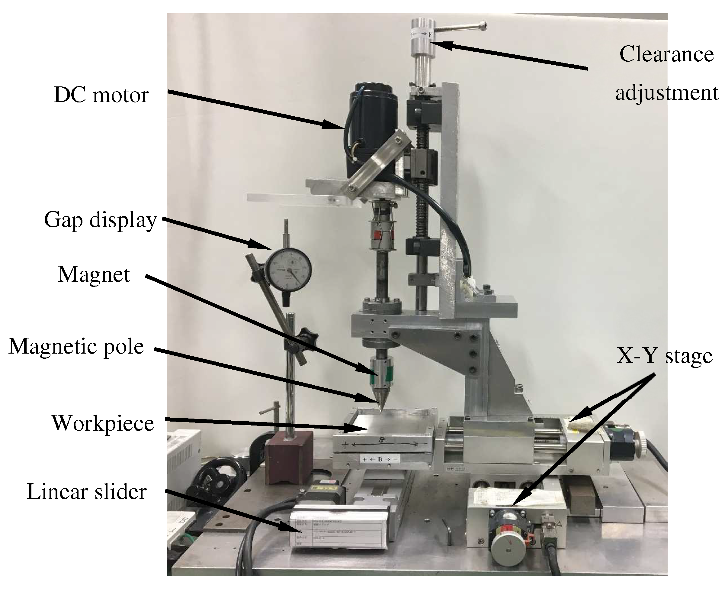
3.1. Experimental Setup
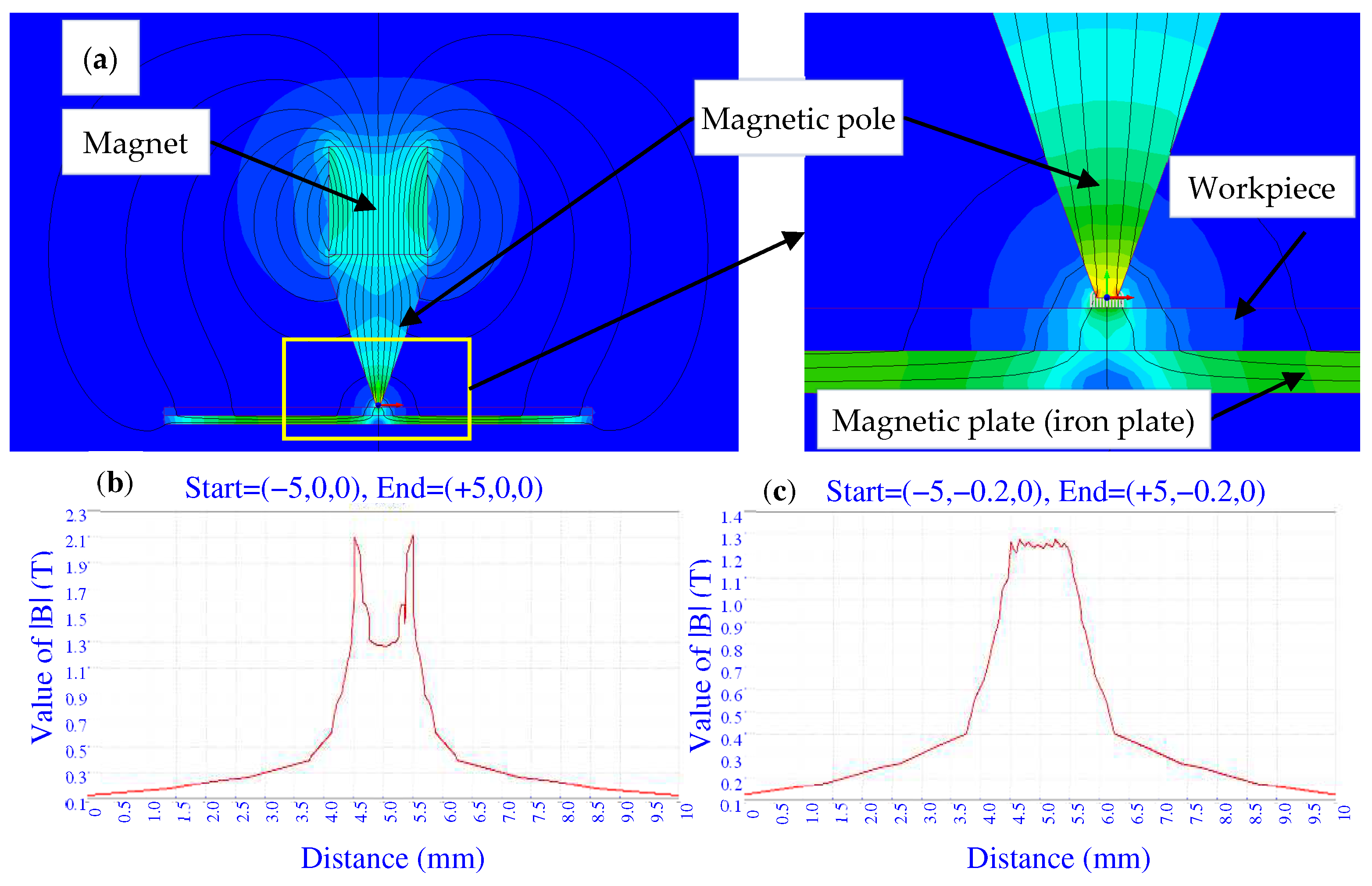
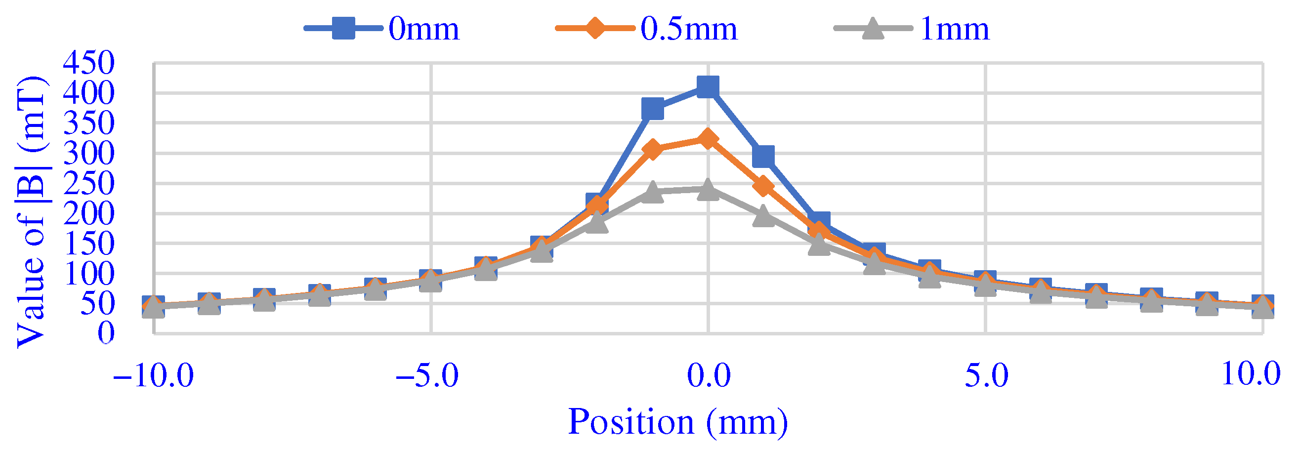
3.2. Magnetic Field Analysis
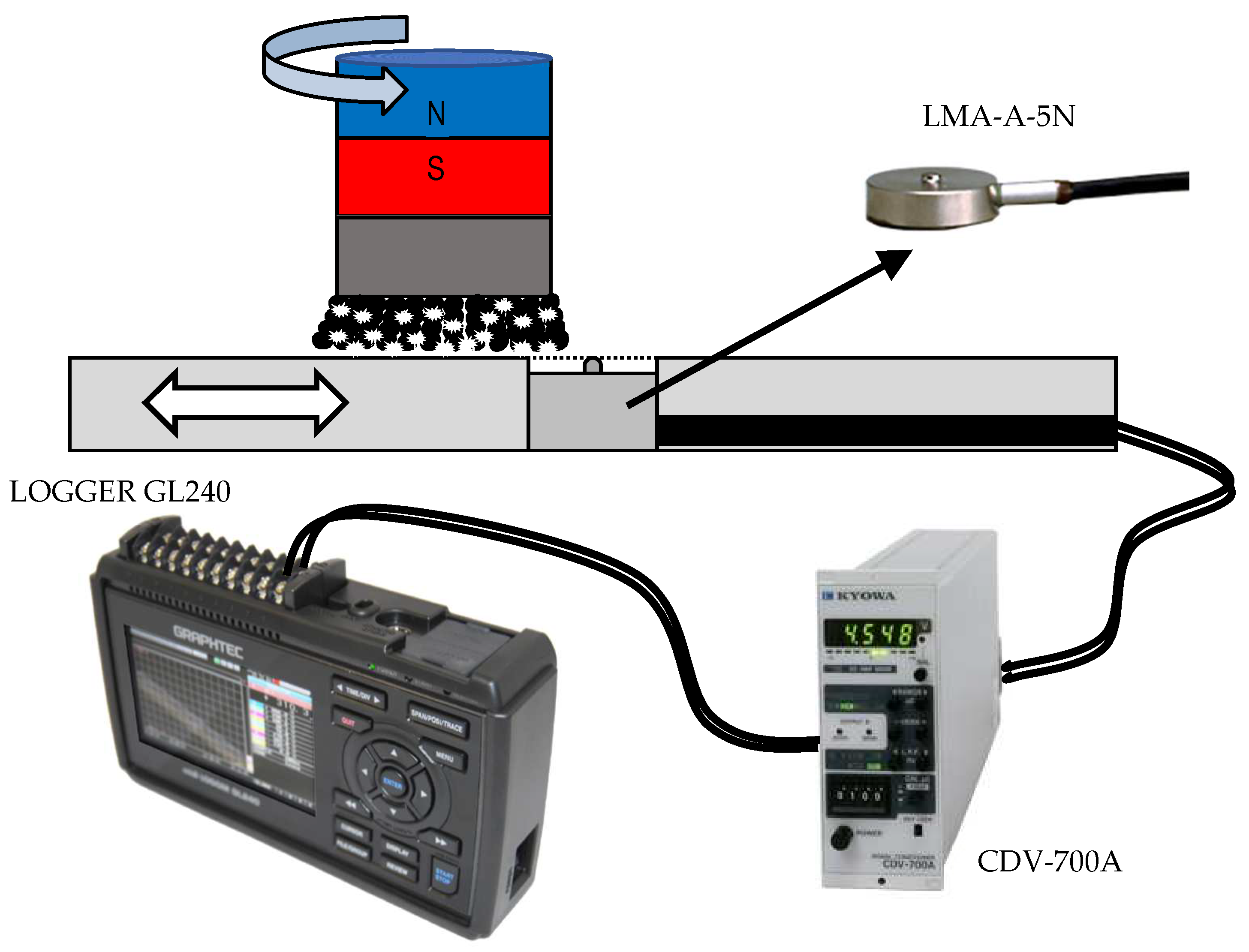
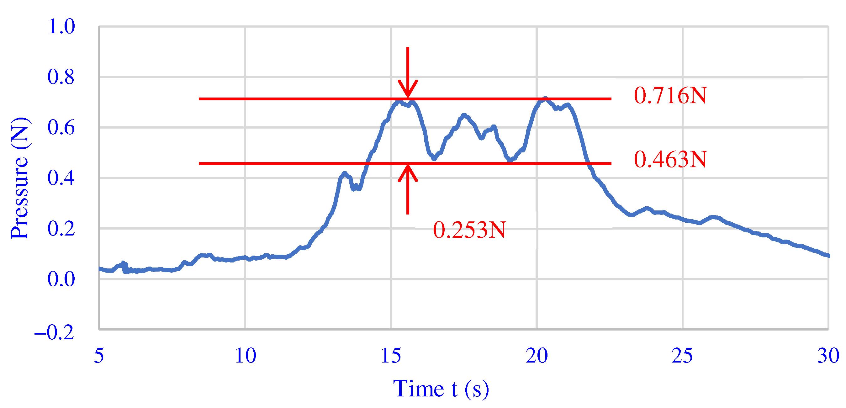
3.3. Force Analysis
4. Experiment and Discussion
- (1)
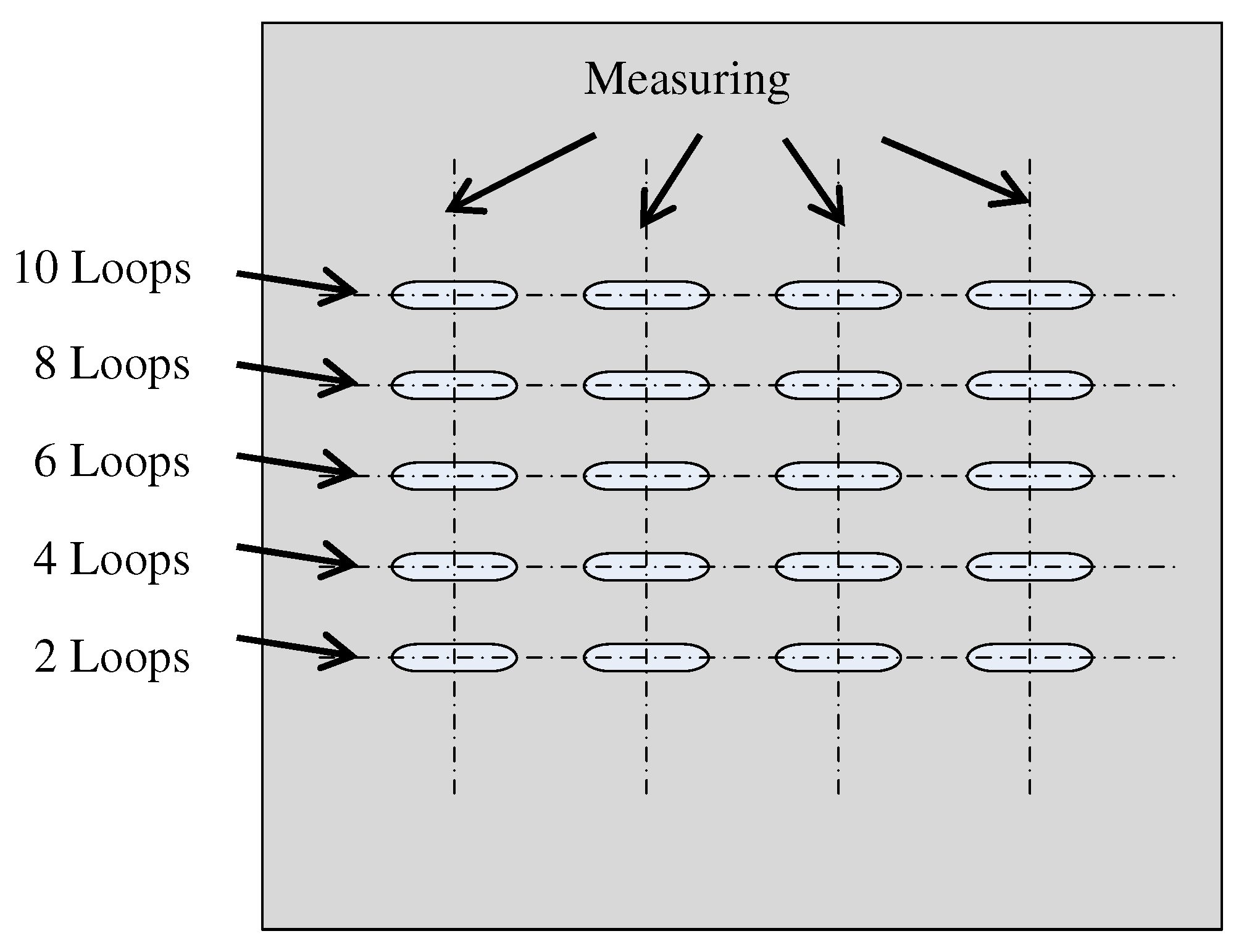
- First, it is necessary to design experiments to calculate the processing efficiency of the magnetic brush, and to obtain the value of ;
- (2)
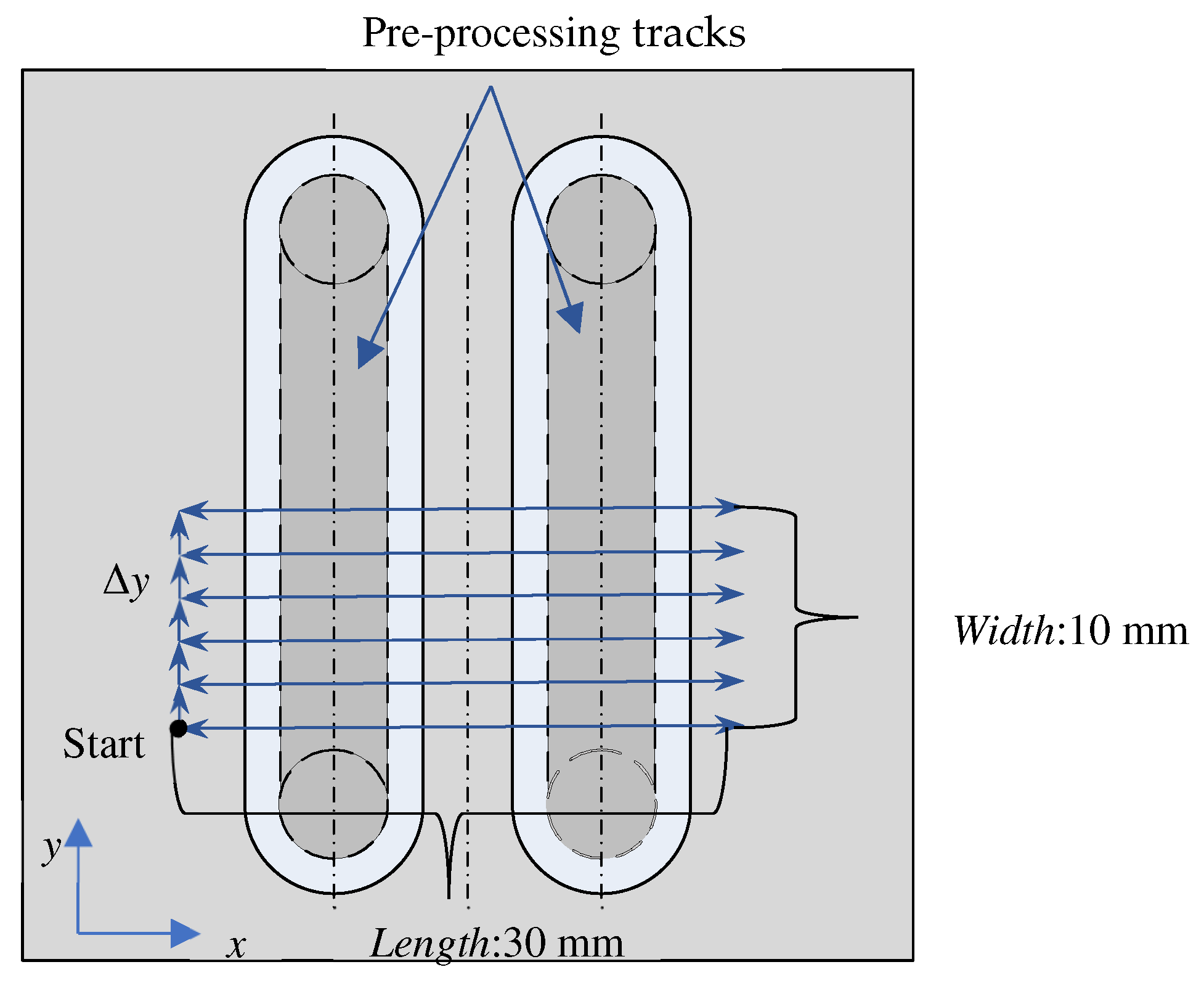
- For Pre-processing, two tracks are processed with a magnetic pole with an end diameter of 3 mm to produce a surface with fluctuation in the x-direction, as shown in Figure 10;
- (3)
- Measuring the profile curves of the workpiece along the x-direction, analyzing and processing the measured data according to the previous method, and obtaining the feed speed curves data during corrective processing;
- (4)
- Corrective processing of the workpiece surface with an area of 30 mm 10 mm ( is 0.5 mm, 1.0 mm, 1.5 mm and 2.0 mm, respectively);
- (5)
- The experimental results are measured and analyzed.
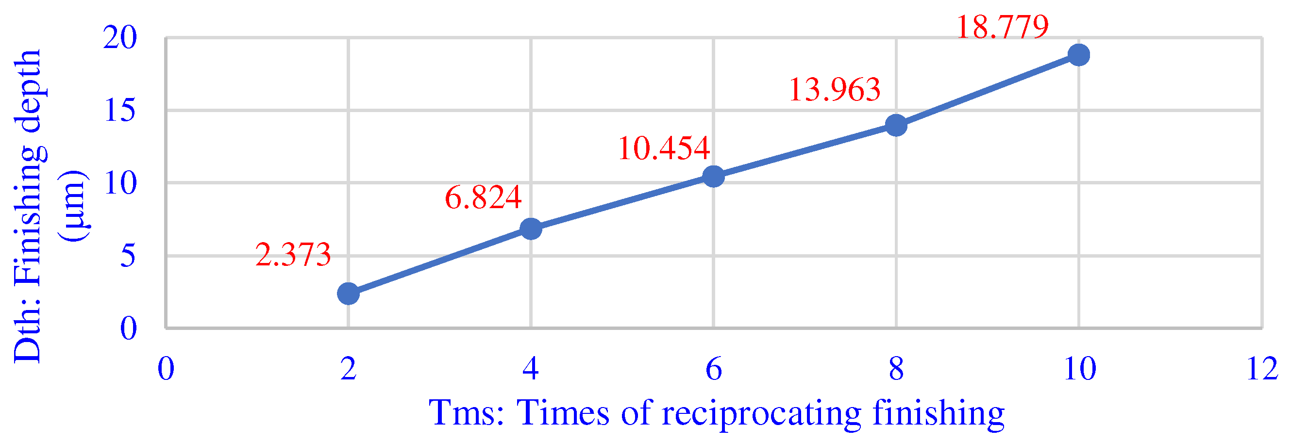
4.1. Magnetic Brush Processing Efficiency Experiments
4.2. Pre-Processing Experiment
4.3. Corrective Finishing Experiments
5. Conclusions
- (1)
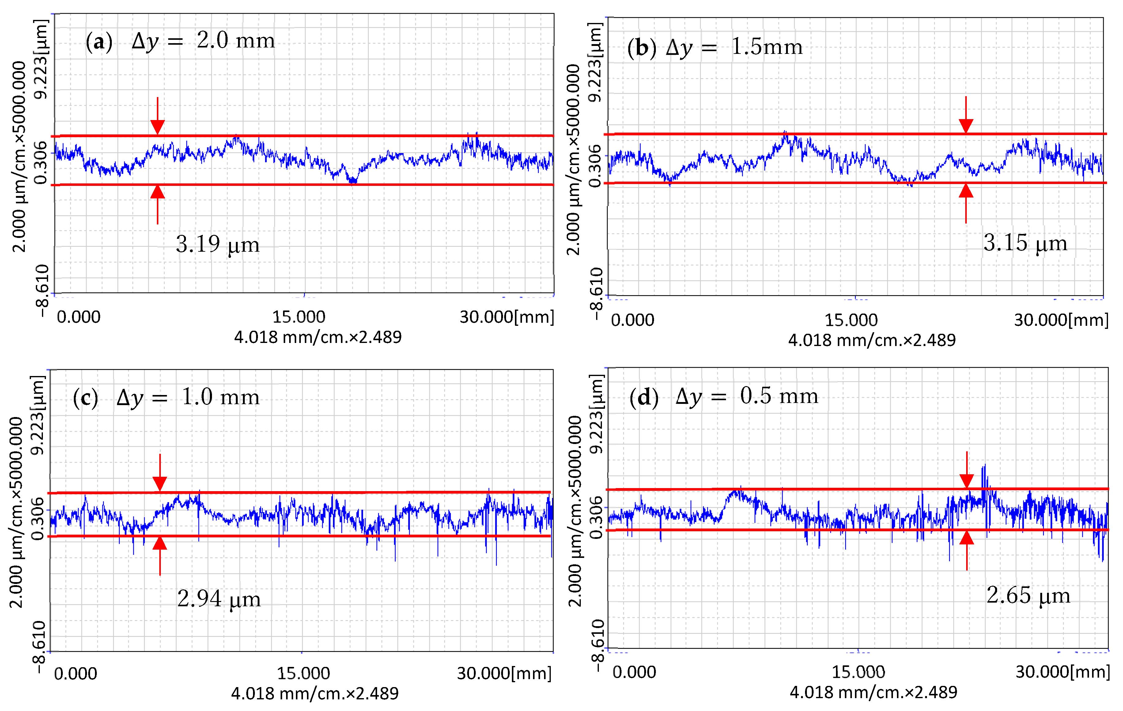
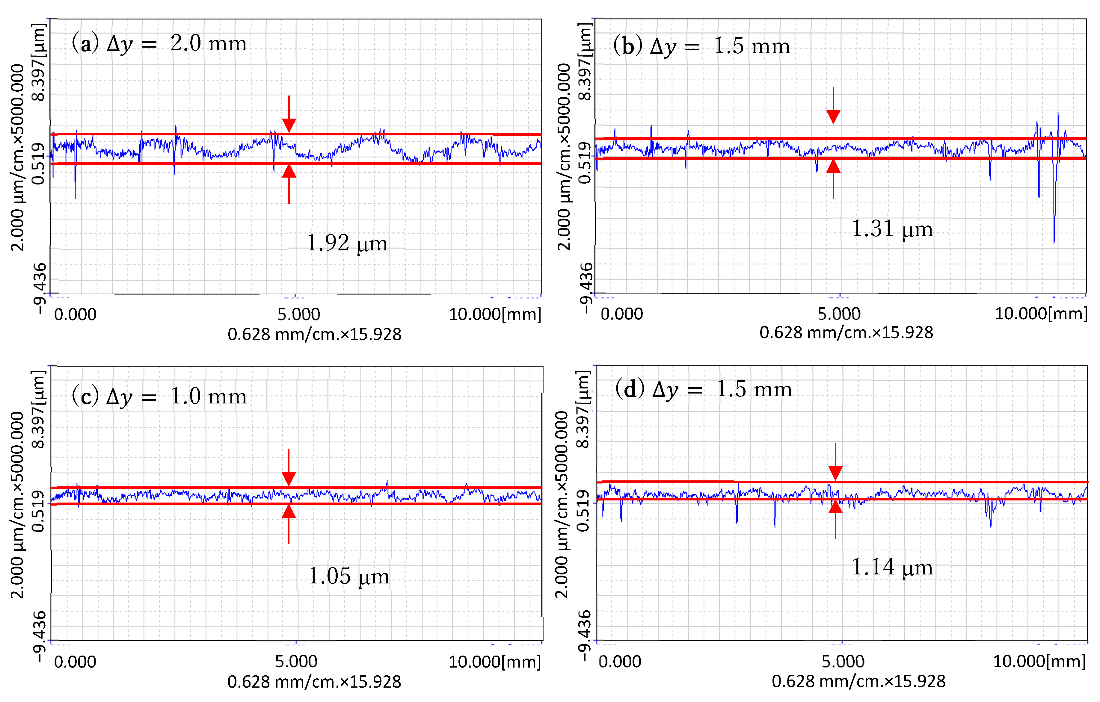
- In the feed direction (-direction), variable speed finishing has an obvious effect on the surface correction. However, when decreases, the processing time becomes longer, so the correction effect is better.
- (2)
- When correcting the surface of the workpiece through speed control, the smaller the step length of the processing track, the smaller the trace of surface transition, but it takes a longer processing time. This experiment proves that the processing effect at 1.0 mm is almost the same as that at 0.5 mm, but the processing time is reduced by half. In variable speed correction finishing, there is a certain correction effect under different conditions, but when is large, it will produce transition traces to the profile in the -direction. When drops to 1.0 mm, the transition traces are almost gone.
- (3)
- The experimental results show that the speed control method can be used to correct the surface profile of the workpiece. The extreme difference can be reduced from 4.81 μm to 2.65 μm within a processed area of 30 mm by 10 mm.
Author Contributions
Funding
Conflicts of Interest
References
- Patil, M.G.; Chandra, K.; Misra, P.S. Magnetic abrasive finishing–A Review. In Advanced Materials Research; Trans Tech Publications Ltd.: Stafa-Zurich, Switzerland, 2012; Volume 418, pp. 1577–1581. [Google Scholar]
- Qian, C.; Fan, Z.; Tian, Y.; Liu, Y.; Han, J.; Wang, J. A review on magnetic abrasive finishing. Int. J. Adv. Manuf. Technol. 2020, 112, 619–634. [Google Scholar] [CrossRef]
- Shinmura, T.; Takazawa, K.; Hatano, E.; Matsunaga, M.; Matsuo, T. Study on magnetic abrasive finishing. CIRP Ann. 1990, 39, 325–328. [Google Scholar] [CrossRef]
- Shinmura, T.; Aizawa, T. Study on magnetic abrasive finishing process-development of plane finishing apparatus using a stationary type electromagnet. Bull. Jpn. Soc. Precis. Eng. 1989, 23, 236–239. [Google Scholar]
- Yamaguchi, H.; Shinmura, T. Study of an internal magnetic abrasive finishing using a pole rotation system: Discussion of the characteristic abrasive behavior. Precis. Eng. 2000, 24, 237–244. [Google Scholar] [CrossRef]
- Zou, Y.H. A new internal magnetic deburring process using a magnetic machining jig-Precise deburring of a drilled hole on the inside of a SUS304 stainless steel tube. J. Jpn. Soc. Abras. Technol. 2007, 51, 696. [Google Scholar]
- Misra, A.; Pandey, P.M.; Dixit, U.S. Modeling of material removal in ultrasonic assisted magnetic abrasive finishing process. Int. J. Mech. Sci. 2017, 131, 853–867. [Google Scholar] [CrossRef]
- Qu, S.; Wang, Z.; Zhang, C.; Ma, Z.; Zhang, T.; Chen, H.; Wang, Z.; Yu, T.; Zhao, J. Material removal profile prediction and experimental validation for obliquely axial ultrasonic vibration-assisted polishing of K9 optical glass. Ceram. Int. 2021, 47, 33106–33119. [Google Scholar] [CrossRef]
- Mulik, R.S.; Pandey, P.M. Ultrasonic assisted magnetic abrasive finishing of hardened AISI 52100 steel using unbonded SiC abrasive. Int. J. Refract. Met. Hard Mater. 2011, 29, 68–77. [Google Scholar] [CrossRef]
- Sun, X.; Zou, Y.H. Development of magnetic abrasive finishing combined with electrolytic process for finishing SUS304 stainless steel plane. Int. J. Adv. Manuf. Technol. 2017, 92, 3373–3384. [Google Scholar] [CrossRef]
- Zou, Y.H.; Xing, B.J.; Sun, X. Study on the magnetic abrasive finishing combined with electrolytic process—Investigation of machining mechanism. Int. J. Adv. Manuf. Technol. 2020, 108, 1675–1689. [Google Scholar] [CrossRef]
- Xing, B.J.; Zou, Y.H. Investigation of finishing aluminum alloy A5052 using the magnetic abrasive finishing combined with electrolytic process. Machines 2020, 8, 78. [Google Scholar] [CrossRef]
- Zou, Y.H.; Satou, R.; Yamazaki, O.; Xie, H.J. Development of a New Finishing Process Combining a Fixed Abrasive Polishing with Magnetic Abrasive Finishing Process. Machines 2021, 9, 81. [Google Scholar] [CrossRef]
- Wu, J.Z.; Zou, Y.H.; Sugiyama, H. Study on finishing characteristics of magnetic abrasive finishing process using low-frequency alternating magnetic field. Int. J. Adv. Manuf. Technol. 2016, 85, 585–594. [Google Scholar] [CrossRef]
- Zou, Y.H.; Xie, H.J.; Dong, C.; Wu, J. Study on complex micro surface finishing of alumina ceramic by the magnetic abrasive finishing process using alternating magnetic field. Int. J. Adv. Manuf. Technol. 2018, 97, 2193–2202. [Google Scholar] [CrossRef]
- Xie, H.J.; Zou, Y.H.; Dong, C.W.; Wu, J.Z. Study on the magnetic abrasive finishing process using alternating magnetic field: Investigation of mechanism and applied to aluminum alloy plate. Int. J. Adv. Manuf. Technol. 2019, 102, 1509–1520. [Google Scholar] [CrossRef]
- Lin, C.T.; Yang, L.D.; Chow, H.M. Study of magnetic abrasive finishing in free-form surface operations using the Taguchi method. Int. J. Adv. Manuf. Technol. 2007, 34, 122–130. [Google Scholar] [CrossRef]
- Zhang, M.D.; Lv, M.; Chen, H.L. Theoretical research on polishing free-form surface with magnetic abrasive finishing. In Key Engineering Materials; Trans Tech Publications Ltd.: Stafa-Zurich, Switzerland, 2009; Volume 392, pp. 404–408. [Google Scholar]
- Maksarov, V.V.; Keksin, A.I. Technology of magnetic-abrasive finishing of geometrically-complex products. In IOP Conference Series: Materials Science and Engineering; IOP Publishing: Bristol, UK, 2018; Volume 327, p. 042068. [Google Scholar]
- Zou, Y.H.; Jiao, A.Y.; Toshio, A. Study on plane magnetic abrasive finishing process-experimental and theoretical analysis on polishing trajectory. In Advanced Materials Research; Trans Tech Publications Ltd.: Stafa-Zurich, Switzerland, 2010; Volume 126, pp. 1023–1028. [Google Scholar]
- Jiao, A.Y.; Quan, H.J.; Li, Z.Z.; Zou, Y.H. Study on improving the trajectory to elevate the surface quality of plane magnetic abrasive finishing. Int. J. Adv. Manuf. Technol. 2015, 80, 1613–1623. [Google Scholar] [CrossRef]
- Zou, Y.H.; Xie, H.J.; Zhang, Y.L. Study on surface quality improvement of the plane magnetic abrasive finishing process. Int. J. Adv. Manuf. Technol. 2020, 109, 1825–1839. [Google Scholar] [CrossRef]
- Preston, F.W. The Theory and Design of Plate Glass Polishing Machines. J. Soc. Glass Technol. 1927, 11, 214–256. [Google Scholar]
- Oh, J.H.; Lee, S.H. Prediction of surface roughness in magnetic abrasive finishing using acoustic emission and force sensor data fusion. Proc. Inst. Mech. Eng. Part B J. Eng. Manuf. 2011, 225, 853–865. [Google Scholar] [CrossRef]
- Zhang, Y.L.; Zou, Y.H. Study of corrective abrasive finishing for plane surfaces using magnetic abrasive finishing processes. Nanotechnol. Precis. Eng. 2021, 4, 033001. [Google Scholar] [CrossRef]
- Kim, D.W.; Kim, S.W. Static tool influence function for fabrication simulation of hexagonal mirror segments for extremely large telescopes. Opt. Express 2005, 13, 910–917. [Google Scholar] [CrossRef] [PubMed] [Green Version]
- Michaeli, W.; Heßner, S.; Klaiber, F.; Forster, J. Geometrical accuracy and optical performance of injection moulded and injection-compression moulded plastic parts. CIRP Ann. 2007, 56, 545–548. [Google Scholar] [CrossRef]


| Workpiece | A5052 plate (100 mm × 100 mm × 2 mm) |
| Magnetic pole | Nd-Fe-B rare earth permanent magnet (Φ1 × 35 mm) |
| Magnetic abrasive | 0.02 g of 149 μm iron powder |
| Abrasion liquid | 0.5 mL of oil (Honilo 988) and 1 g of #4000 WA particles |
| Clearance | 0.2 mm |
| Finishing distance | 6 mm |
| Finishing loops | 2-4-6-8-10 loops |
| Feed speed | 0.2 mm s−1 |
| Rotation speed | 400 r min−1 |
| Workpiece | A5052 plate (100 mm × 100 mm × 2 mm) |
| Magnetic pole | Nd-Fe-B rare earth permanent magnet (Φ3 × 35 mm) |
| Magnetic abrasive | 0.5 g of 149 μm iron powder |
| Abrasion liquid | 0.5 mL of oil (Honilo 988) and 1 g of #4000 WA particles |
| Clearance | 0.2 mm |
| Finishing distance | 80 mm |
| Finishing time | 40 min |
| Feed speed | 0.5 mms−1 |
| Rotation speed | 400 rmin−1 |
Publisher’s Note: MDPI stays neutral with regard to jurisdictional claims in published maps and institutional affiliations. |
© 2022 by the authors. Licensee MDPI, Basel, Switzerland. This article is an open access article distributed under the terms and conditions of the Creative Commons Attribution (CC BY) license (https://creativecommons.org/licenses/by/4.0/).
Share and Cite
Zhang, Y.; Zou, Y. Study on Corrective Abrasive Finishing for Workpiece Surface by Using Magnetic Abrasive Finishing Processes. Machines 2022, 10, 98. https://doi.org/10.3390/machines10020098
Zhang Y, Zou Y. Study on Corrective Abrasive Finishing for Workpiece Surface by Using Magnetic Abrasive Finishing Processes. Machines. 2022; 10(2):98. https://doi.org/10.3390/machines10020098
Chicago/Turabian StyleZhang, Yulong, and Yanhua Zou. 2022. "Study on Corrective Abrasive Finishing for Workpiece Surface by Using Magnetic Abrasive Finishing Processes" Machines 10, no. 2: 98. https://doi.org/10.3390/machines10020098