Article

3D-FEM Approach of AISI-52100 Hard Turning: Modelling of Cutting Forces and Cutting Condition Optimization

by
Anastasios Tzotzis
1,
Nikolaos Tapoglou
2,
Rajesh Kumar Verma
3 and
Panagiotis Kyratsis
1,*
1
Department of Product and Systems Design Engineering, University of Western Macedonia, Kila, 50100 Kozani, Greece
2
Department of Industrial Engineering and Management, International Hellenic University, Sindos, 57400 Thessaloniki, Greece
3
Department of Mechanical Engineering, Madan Mohan Malaviya University of Technology, Gorakhpur 273010, India
*
Author to whom correspondence should be addressed.
Machines 2022, 10(2), 74; https://doi.org/10.3390/machines10020074
Submission received: 18 December 2021 / Revised: 11 January 2022 / Accepted: 18 January 2022 / Published: 20 January 2022
(This article belongs to the Special Issue Feature Papers to Celebrate the First Impact Factor of Machines)

Abstract

:
In the present study, a 3D finite element (FE) model for machining AISI-52100 steel was proposed, with respect to three levels of cutting speed (100 m/min, 150 m/min and 200 m/min), feed (0.08 mm/rev, 0.11 mm/rev and 0.14 mm/rev), depth of cut (0.20 mm, 0.30 mm and 0.40 mm) and tool nose radius (0.80 mm, 1.20 mm and 1.60 mm). Nine simulation tests were performed according to cutting conditions that were used in experimental studies, in order to verify the accuracy of the model. Next, the FE model was utilized to carry out thirty new simulation runs, with cutting conditions derived from the implementation of the central composite design (CCD). Additionally, a mathematical model was established for prediction purposes, whereas the relationship between the applied cutting parameters and their influence on the resultant cutting force was investigated with the aid of statistical methodologies such as the response surface methodology (RSM) and the analysis of variance (ANOVA). The comparison between the numerical and the statistical model revealed an increased level of correlation, superseding 90% in many tests. Specifically, the relative error varied between −7.9% and 11.3%. Lastly, an optimization process was performed to find the optimal cutting conditions for minimizing the resultant machining force, as per the standardized tool nose radius value.

1. Introduction

Machinability of hardened materials, and especially of hardened steels, is an aspect that is widely studied, since these materials are repeatedly used by the manufacturing industry to produce standardized machine elements such as bearings. Thus, the availability of established models for the machining of such materials in a broad range of cutting conditions is crucial. Use of finite element (FE) models is one way to achieve this goal. Despite the fact that FE modelling can be time-consuming, even with the use of modern computers, it is a method that provides multiple benefits to the researcher such as visualization of the experimental process, good approximation of complex problems, adaptability and the ability to yield multiple output data [1].
Early studies on machining with the aid of the finite element method (FEM) was carried out by Klocke et al. [2], who investigated 2D orthogonal high speed cutting of AISI-1045 steel. Huang and Liang [3] established a 2D FE model for modelling cutting forces during hard turning of AISI-52100 steel, considering tool wear also. More recently, Yaich et al. [4] studied the effects of the constitutive coefficients on FE models of Ti6Al4V 2D orthogonal cutting. Yameogo et al. [5] employed FEM in two dimensions to predict cutting forces and chip morphology when machining Ti6Al4V. Similar studies are available for aluminum alloys as well. Seshadri et al. [6] developed a 2D FE model for the orthogonal cutting of Al2024-T351 alloy. Zhou et al. [7] performed 2D simulations to optimize the cutting parameters during machining of aluminium–silicon alloy ZL109 with polycrystalline diamond (PCD) cutting tools. Chiappini et al. [8] investigated the mechanics of chip formation during Ti6Al4V alloy machining with spindle speed variation.
Even though 2D FE modelling can be particularly useful in certain cases due to its simplicity, it lacks the ability to approximate complex problems. For that, researchers opt to model in 3D when necessary. The 3D FEM is applied in almost every machining process, especially in typical processes such as drilling, turning and milling. Miller and Shih [9] modelled friction drilling of Al6061-T6 through an explicit FEM code with temperature-dependent mechanical and thermal properties. Nan et al. [10] studied the three-dimensional FE modeling for simulating the small-hole drilling process of AISI-1045 steel by using ABAQUS™ software. Similar studies were conducted with the aid of other finite element analysis (FEA) systems, such as DEFORM™-3D [11,12,13,14]. These studies investigate the generated thrust forces, the chip formation and tool life for industrial materials, such as titanium alloy Ti6Al4V, aluminium alloy Al7075-T6 and AISI-4340 steel.
Another typical machining process that is often studied with the aid of FEM is milling. Thepsonthi and Özel [15] investigated micro-end milling processes of Ti-6Al-4V via 3D FE modelling. Authors proposed models for full immersion and half immersion up and down milling in order to study the influence of several aspects during this process. Additionally, they provided a comparison between 2D and 3D simulations. Gao et al. [16] established a 3D coupled Eulerian–Lagrangian FE model for simulating end milling processes by using ABAQUS™ software. The selected milling techniques in the proposed model are slot and shoulder milling of aluminum alloy Al6061-T6. Similarly to drilling, the selected materials for investigation are usually typical materials that are used by manufacturing industries such as aerospace, automotive, defense and energy. Moreover, estimation of the generated cutting forces, chip development, the temperature of the chip-workpiece interface and tool wear are some of the most studied parameters during milling [17,18].
Since turning is one of the most used machining processes, the application of 3D FEM in research related to turning is no exception. Valiorgue et al. [19] presented the development of a new methodology for predicting the residual stresses induced in finish turning of AISI304L stainless steel. To do so, the authors followed a hybrid approach by combining experimental testing and numerical modelling. Liu et al. [20] determined the Johnson–Cook constitutive material model for stainless steel 17-4PH with the aid of an orthogonal cutting model and inverse analysis in order to develop an FE model for force predictions. In addition, authors investigated the performance of micro-grooved tools with the aid of 3D FE modelling. Lotfi et al. [21] modelled conventional turning, rotary turning and ultrasonic-assisted rotary turning of AISI-4140 steel in three dimensions, to predict tool wear and heat distribution on tool faces. Similar works were carried out to predict several critical parameters in turning, such as the resultant machining force, the temperature distribution on the workpiece-tool interface, the residual stresses, the tool wear and the chip morphology [22,23,24,25].
In the present study, the effects of typical machining conditions on the resultant cutting force are investigated with the aid of a three-dimensional FE model. The test setup includes four cutting parameters in three levels, whereas the selected test workpiece and cutting tools are AISI-52100 steel and SNGA inserts with three different nose radii, respectively. In order to produce the required number of tests, the central composite design (CCD) was employed, leading to 30 tests. The development of the 3D FE model and the equivalent simulations were performed with DEFORM™-3D ver. 12 software. Moreover, prior to the realization of the 30 simulations, a set of nine simulations were carried out for verification purposes of the model. To do so, a comparison was made with experimental results. In addition, a mathematical model was developed by the numerical results and verified accordingly, so that future experimental work can be minimized, providing the possibility also to extend the range of cutting conditions. Finally, a response optimization was performed in order to find the optimal cutting conditions for each one of the cutting tools used.

2. Materials and Methods

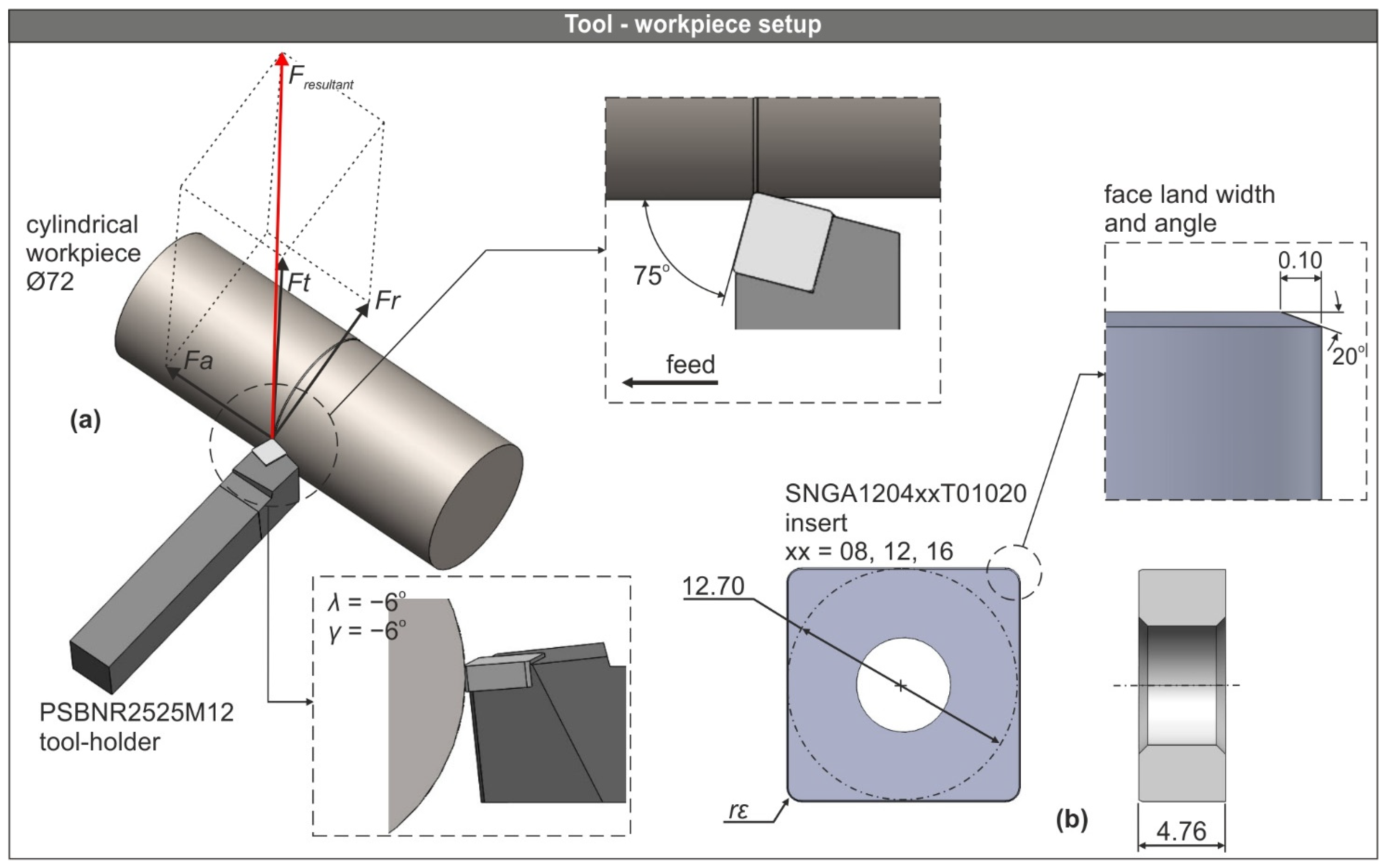
2.1. CAD-Based Setup of the Machining Process

A CAD-based setup was realized in SolidWorks™ 2021 in order to analyze important parameters of the AISI-52100 steel machining process, such as the cutting area, the contact points between the tool and the workpiece and the machining forces vectors. The purpose of this procedure was to develop a simplified analysis domain that can be used to facilitate the building process of the FE model.
The tool assembly used in this work comprises a tool-holder with ISO designation PSBNR2525M12 and three versions of a standard square-shaped turning insert with ISO codes SNGA120408T01020, SNGA120412T01020 and SNGA120416T01020, respectively. The workpiece model was designed to be cylindrical with a diameter equal to 72 mm. In addition, the workpiece and insert material in the present study were AISI-52100 steel and ceramic, respectively.
Figure 1a depicts the models of the workpiece and the tool assembly, as well as the vectors of the generated machining forces: Ft corresponds to the tangential force, Fr is the radial force and Fa represents the feed force. Additionally, Figure 1a illustrates the contact point of the tool on the cutting surface with the aid of two extra schematics, revealing the lead angle, the rake angle, as well as the inclination angle. The values of these angles are drawn from the geometry of both the tool-holder and the insert. According to the specifications of the tool-holder and the insert, the lead angle was 75°, whereas the rake and the inclination angles were both equal to −6°. Furthermore, Figure 1b illustrates the geometry and the characteristics of the turning inserts used. The face land width and the face angle are the same for all three inserts, and were equal to 0.10 mm and 20°, respectively. Moreover, the tool nose radius (rε) was 0.80 mm, 1.20 mm and 1.60 mm, according to the ISO code of each insert. Lastly, the SNGA-ceramic inserts are typically used for machining cast iron and hardened steel.
A total of thirty-nine simulation tests were carried out in the present study. Nine tests were used to verify that the numerical model presented in this work is correlated with the equivalent experimental tests that are available in the literature [26], whereas thirty tests were used to build a statistical model for prediction purposes of the resultant machining force during turning of AISI-52100 steel. Table 1 contains the factors along with their levels, which were used in the present study. Specifically, the four factors were the cutting speed (Vc), the feed (f), the depth of cut (ap) and the tool nose radius (rε), each in three levels.

2.2. Pre-Processing of the Numerical Model

In order to achieve reasonable simulation times, the CAD-based setup was used to model a simplified version of the workpiece and tool. As seen in Figure 2, the workpiece was modelled to be a 20° section of the workpiece that belongs to a Ø72 cylinder. The geometry of the section was chosen according to the tool nose radius and the depth of cut applied in each test, forming a pre-cut surface that represents the geometry of the machined surface and further improves the simulation time.

2.2.1. Analysis Interface Specifications

The models of the workpieces were designed in SolidWorks™ 2021 and modelled in DEFORM™-3D ver.12 as deformable with a mesh of approximately 60,000 to 120,000 tetrahedral elements according to the applied value of feed. The minimum element size of the mesh was set to 25% of the feed [22,27]. In addition, the ratio of the size between the largest and the smallest element of the mesh was set to 7:1, which is the default value given by the software. The purpose of this technique is to create a denser mesh at the section of the workpiece (see Figure 2b), especially at the contact area between the tool nose and the surface of the workpiece, where the element removal occurs. In contrast, the tools used were modelled to be rigid, with the mesh having the maximum available number of elements, which is approximately 50,000. Even though the mesh of the tool does not have a significant effect on the generated results, a denser mesh provides better visualization of the process with minimal change of the simulation time. Similar to the workpiece, the tool nose area that is in contact with the workpiece was refined with a 4:1 ratio (see Figure 2c), which is again the default value. Finally, in order to maintain a minimum number of elements at the mesh during the chip creation process, the embedded-to-the-software remeshing technique was applied with the next criteria: local remeshing with size control based on the average size of the surrounding elements of the distorted mesh.
The workpiece’s model was fixed to set the translational boundary conditions, whereas the cutting tool was set to follow the cutting path pointed out in Figure 2a. Additionally, to set the thermal boundary conditions, the heat exchange due to convection and conduction of both the workpiece and the cutting tool to the ambient environment (temperature equal to 20 °C) were also set by applying the equivalent coefficients as suggested by DEFORM™ [28]. For dry conditions, these coefficients are: hconv = 0.02 N/(s × mm × °C) and hcond = 45 N/(s × mm × °C), respectively.

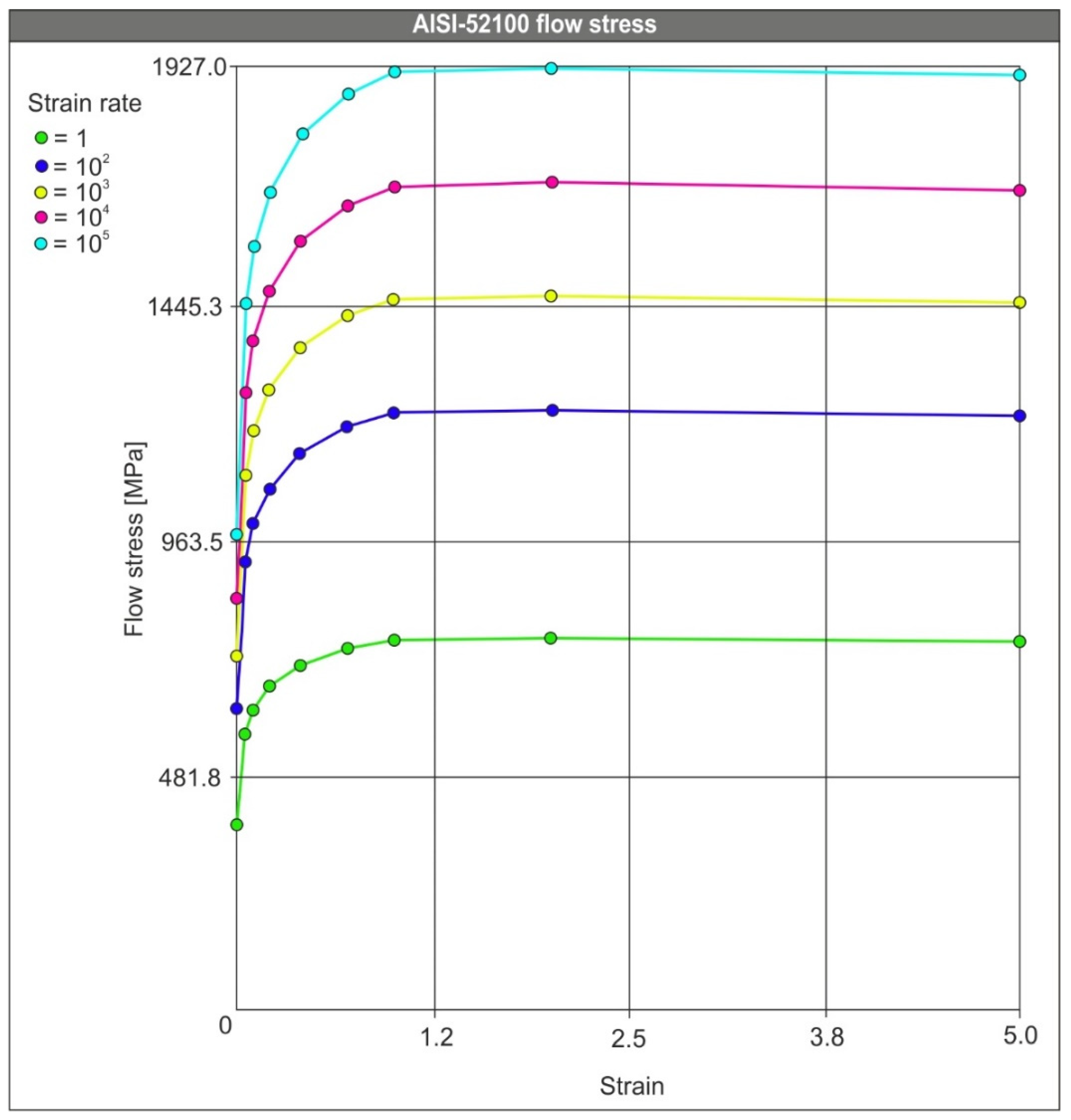
2.2.2. Material Modelling

Even though many material models exist in the literature, a tabular data format is implemented in the present study in order to model the material flow stress, since it is the most versatile format. The tabular format can represent many materials, as long as the flow stress is a function of strain, strain rate and temperature. Equation (1) represents the material flow stress.
σ ¯   =   f ( ε ¯ , ε ¯ ˙ , T )
where: σ ¯ is the flow stress in MPa, ε ¯ is the effective plastic strain, ε ¯ ˙ represents the effective strain rate and finally T is the temperature in °C.
Flow stress values for AISI-52100 can be interpolated in log strain, log strain rate and linear temperature space in order to generate flow stress diagrams [28] that are similar to the one illustrated in Figure 3, which is generated at 20 °C.
Table 2 contains the thermo-mechanical properties of the materials for both the workpiece and tool. Moreover, both the thermal conductivity and the heat capacity were expressed as a function of temperature f(T).
The selected damage model for this work was the normalized Cockcroft–Latham damage model. This model has been employed by many early studies [30,31,32] for the calculation of damage during material separation. Equation (2) represents the modified criterion developed by Cockcroft and Latham [33], where the maximum principal stress is normalized by the effective stress.
D c   =   0 ε f σ m a x σ ¯ d ε p l
where: Dc is the critical value of the damage during fracture; σmax and σ ¯ represent the maximum tensile principal stress and the effective stress, respectively; εf denotes the limit fracture strain; εpl is the plastic strain.
Regarding the friction modelling, Coulomb’s law was employed in order to approximate the frictional stresses that occur during the contact between the tooltip and the surface of the workpiece. The contact area is divided into three zones: sticking, adhesion and sliding [34]. Since the sliding zone is of great importance when studying the machining of steel and provides a good approximation of the phenomena, it was implemented in the present work. Equation (3) represents the generated stresses in the sliding zone [34].
τ f   =   μ σ n
where: τf is the frictional shear stress; μ denotes the shear friction coefficient, whereas σn represents the stress developed on the tool-chip interface. A number of similar studies on the machining of different types of steel [35,36] suggest applying a friction coefficient between −0.5 and 0.6. Moreover, the friction coefficient value that DEFORM™ proposes is 0.6, which was also the selected value for the simulation runs included in the present study.

3. Results and Discussion

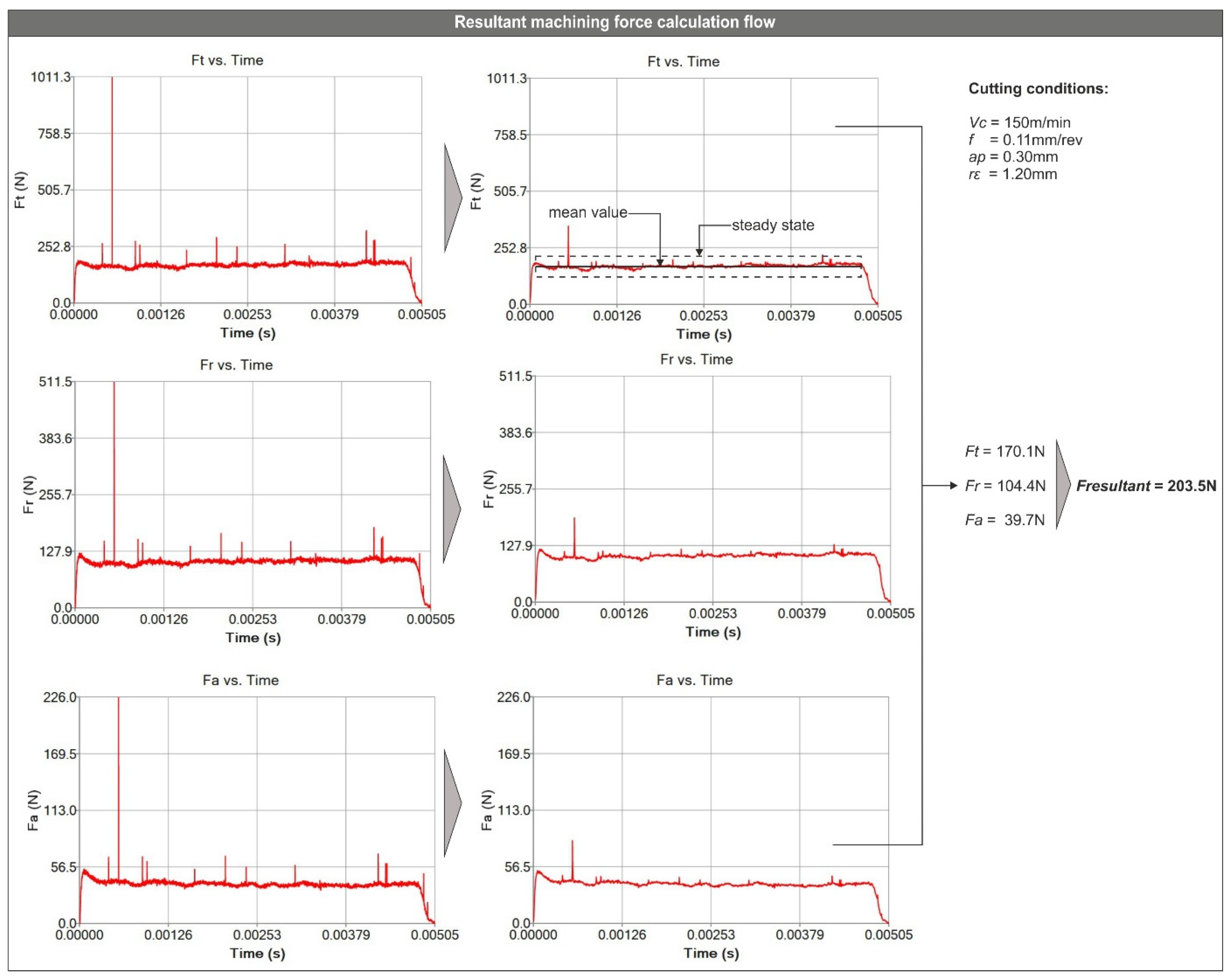
3.1. FEM-Based Evaluation of the Resultant Cutting Force

Nine simulation runs were carried out in order to determine the accuracy of the developed FE model. To do so, the results of these tests were compared to the equivalent experimental values of machining forces for the same cutting conditions. To simplify the processing of the results, the resultant machining force was calculated using the yielded values of the tangential, the radial and the feed force, with the aid of Equation (4). Moreover, the resultant force will always be higher compared to any of the three components; thus, it is safer to use it for prediction purposes of other parameters (i.e., tool wear).
F r e s u l t a n t   =   F t 2   +   F r 2   +   F a 2
where: Fresultant is the resultant machining force in N, Ft represents the tangential force in N, Fr is the radial force in N and Fa denotes the feed force in N.
Table 3 includes the results of the machining force that the numerical model yielded, as well as the experimental values and the relative error. Although some discrepancies occurred during the comparison between the experimental and the simulated forces, they still remained reasonable considering the precision that the FEM can offer, with the relative error varying between −1.7% and 16.7%.
To obtain the values for each one of the force components, each force vs. time diagram was cleared from any unrealistic values by applying first order exponential smoothing. Next, the force values that were generated after the steady state had occurred were used to calculate the mean value. Finally, the resultant machining force was calculated with Equation (4), as mentioned above. Figure 4 presents the flow for determining the resultant force for an indicative simulation run (number 4–Table 4).
Furthermore, it is noted that similar works [37,38] reported cutting forces of the same magnitude for similar cutting conditions and processes such, as AISI-D2 steel turning with the CNGA120408T0120 ceramic tool at 0.2 mm depth of cut and AISI-52100 steel turning with the SNGA120408 ceramic tool at 0.5 mm depth of cut, accordingly. The experimental tests that were recreated were selected in such a way so that a variety of cutting conditions was formed in three levels: one lower level, one mid-level and one upper level (see Table 1). For instance, the three levels for feed are 0.08 mm/rev, 0.11 mm/rev and 0.14 mm/rev, accordingly. Finally, it is noted that these tests were performed in a constant depth of cut equal to 0.25 mm.

3.2. Mathematical Modelling of the Resultant Cutting Force

Next, to study the effects of the cutting conditions and the interaction between them, a set of thirty new simulation runs were carried out according to the number of factors and their levels involved in the study. To determine the number of the tests, the order and the combination of the factors, a Box-Wilson CCD was implemented. CCD is the most commonly used design for response surface methodology (RSM), which is a factorial or fractional factorial design with center points, enhanced with a group of axial points that can estimate the curvature. A CCD is usually used to efficiently estimate first and second-order terms, as well as to model a response variable with curvature by adding center and axial points to an already ready factorial design. This method was employed by many researchers [26,39,40] for similar studies related to different machining processes of steel and other materials used in industry, due to its versatility.
In this study, the runs are composed of 16 factorial points, 6 center points and 8 axial points; additionally, the value of α is equal to 1. As indicated by Table 1, the independent variables (input) are: cutting speed (Vc), feed (f), depth of cut (ap) and tool nose radius (rε), whereas the response (output) is the resultant cutting force (Fresultant).
In addition to the 3D FE model, a statistically-based model was developed by using the CCD build and the numerical results. The benefits that derive from the use of such a model are the reduced number of required simulation runs and the instant prediction of the responses under a wider range of input values, always within the limits of the study. The generated model is a second order polynomial that is described by Equation (5). Since the interaction between the inputs and the response is non-linear, the polynomial includes linear, quadratic, and cross-product terms.
Y   =   a 0   +   i = 1 n b i X i   +   i , j n b i j X i X j   +   i = 1 n b i i X i 2
where: Y is the response of the model (resultant machining force), a0 denotes the fixed term, Xi represent the input variables (cutting speed, feed rate, depth of cut and tool nose radius) and, finally, bi, bij, and bii relate to the vectors that contain the regression coefficients (linear, quadratic, and cross-product, accordingly).
Equation (6) describes the complete statistical model that can be used to predict the resultant machining force according to Equation (5) and the data generated by the FE model (see Table 4).
F r e s u l t a n t   =   118 0.474 V c 6374 f   +   1631 a p   +   136 r ε   +   0.0016 V c 2   +   30059 f 2 2341 a p 2 46.3 r ε 2 + 0.17 V c f 0.445 V c a p 0.018 V c r ε   +   3106 f a p 142 f r ε   +   42.1 a p r ε
Table 4 contains the full set of the designed tests with the applied cutting parameters, as well as the predicted values of the resultant cutting force derived from both the FE model and the statistical one. The relative error ranges between −7.9% and 11.3%, indicating a good correlation between the two models.

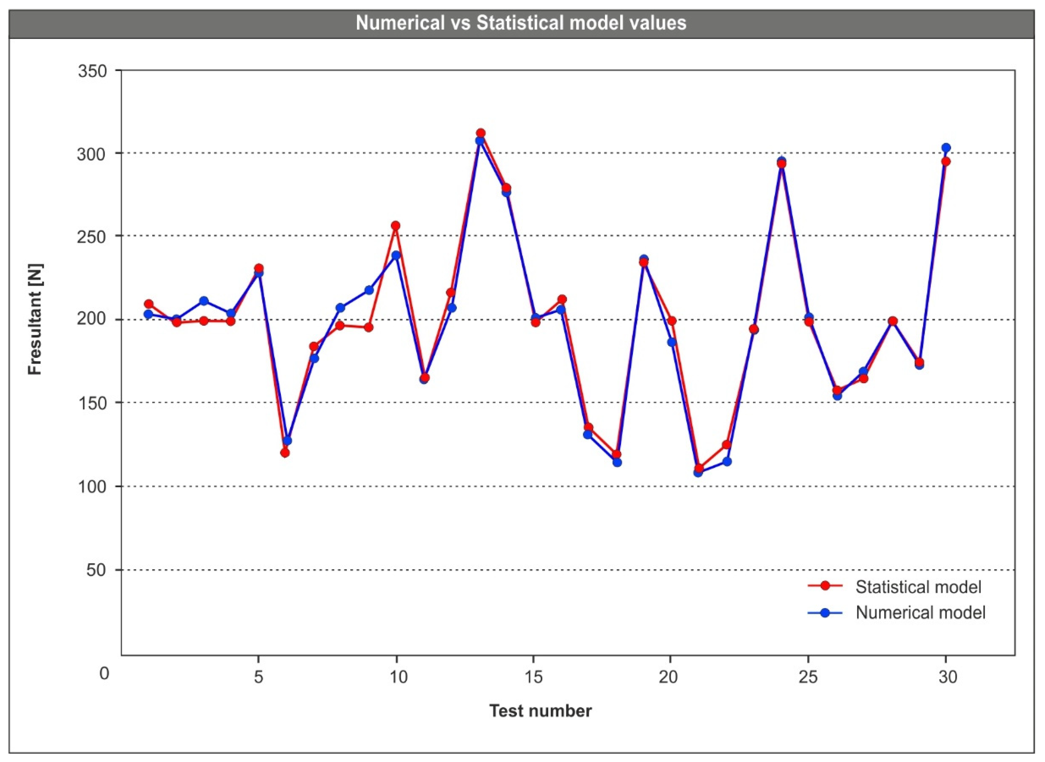
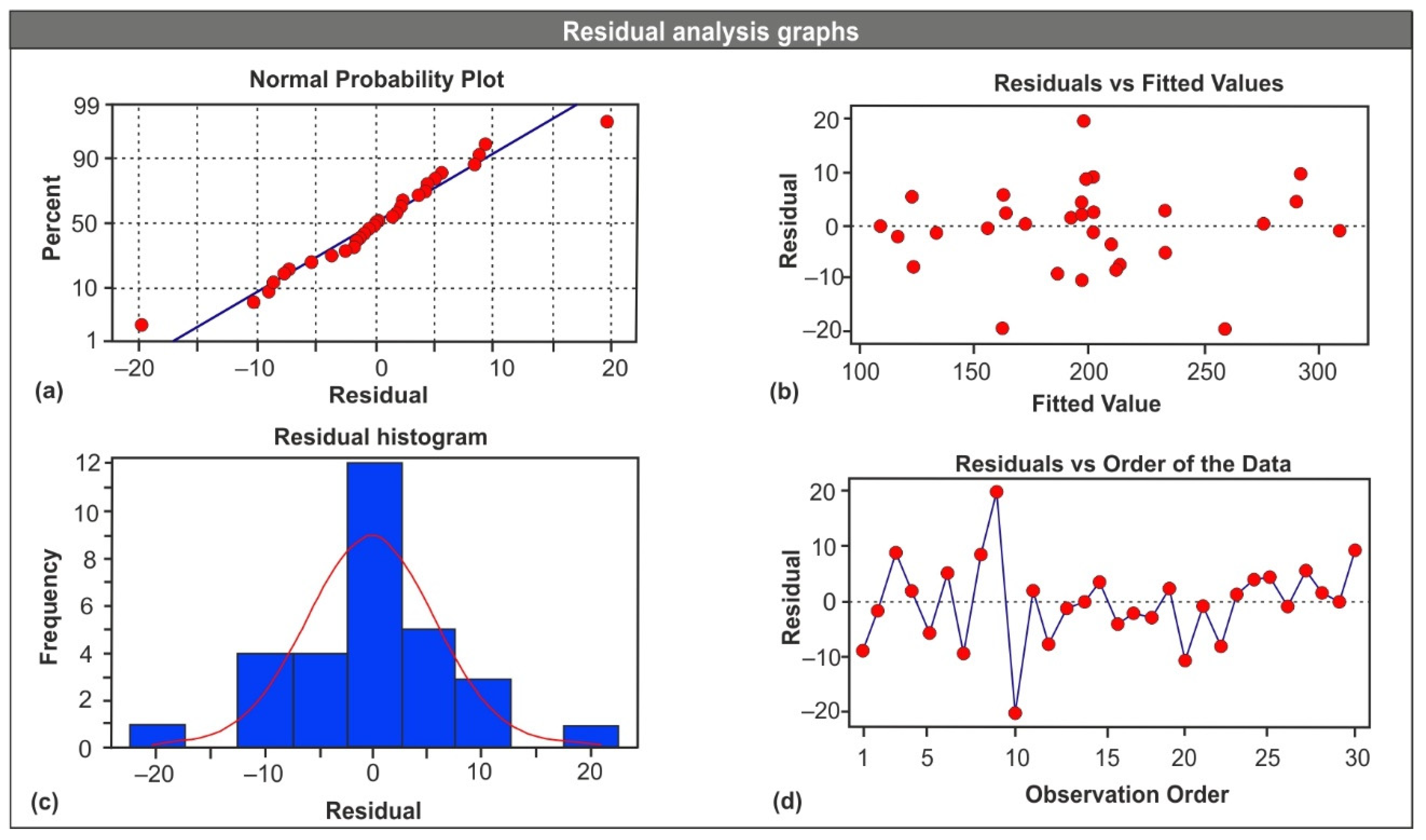
3.3. Analysis and Validation of Mathematical Model

The curves of the simulated and the predicted values of the resultant cutting force are plotted in Figure 5. It is visible that the blue curve fits the red one, with the exception of some points where a small divergence is noticeable, signifying the accuracy of the statistical model.
To assess the importance of the factors, thus validating the model, the analysis of variance (ANOVA) was utilized with a significance level of α = 0.05. The analysis yielded an adjusted R-squared of 95.85%, meaning that the fit of the model is good. The obtained ANOVA results are presented in Table 5, where the p-value can be used to examine the significance of each of the parameters. It is noted that, with the selected significance level, every factor with a p-value below 0.05 (p-value ≤ α) is considered statistically significant and contributes to the model. Hence, the next terms: Vc, f, ap, rε, f2, ap2 and f × ap contribute the most to the model, indicating the strong influence of the four cutting parameters on the generated forces, especially of the feed and the depth of cut. Additionally, the variation of the response, can be graphically presented with the aid of the graph of Figure 6a, as well as expressed with the total sum of squares. Finally, the p-value (zero) of the model itself indicates that the chances of producing abnormal results are rather low.
The residual analysis is graphically presented in Figure 6. In particular, Figure 6a illustrates the normal probability plot where the distance of the data points from the fit line is shown. The closest to the line, the better the fit of the model. Figure 6a suggests that the current fit is good. The plot of Figure 6b depicts the residuals versus the fitted values. This plot shows the distribution of the residuals compared to the reference line. The present study indicates that the residuals are almost evenly distributed on both sides of the reference line. The histogram of Figure 6c presents the residual distribution in the model. According to Figure 6c, the residual values are uniformly distributed and a fit line can be plotted. Finally, Figure 6d depicts the residuals versus the order of the data. This plot can prove the normality of the system. Specifically, the randomized pattern (no trend, no clustering) of the chart proves that no systematic faults are present in the system.

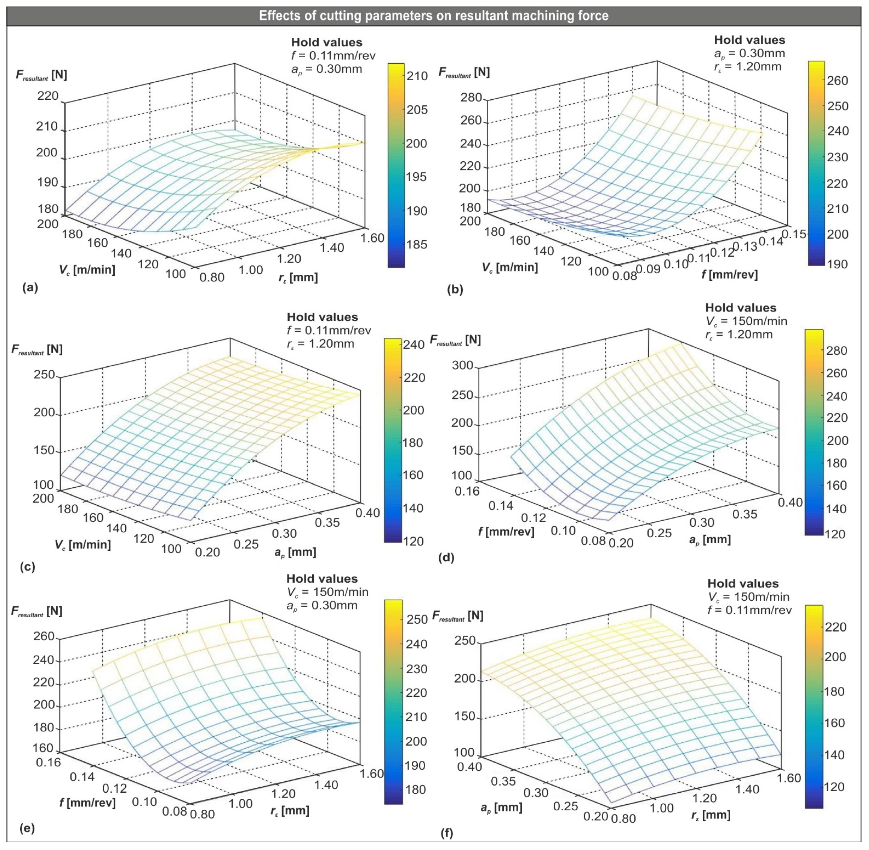
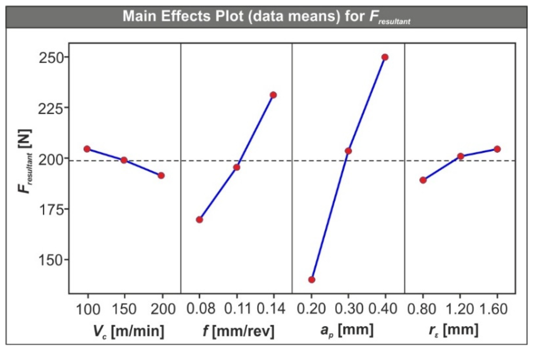
3.4. Investigation of the Cutting Parameters’ Influence

The combined effect of the applied cutting conditions can be illustrated with the aid of 3D surface graphs, according to the polynomial solutions, as shown in Figure 7. Specifically, the effect of both cutting speed and tool nose radius is depicted in Figure 7a where it is noted that, as cutting speed increases, the generated force is reduced. At the same time, tool nose radius acts increasingly on the cutting force, especially when it is increased from 0.80 mm to 1.20 mm. On the contrary, an increase from 1.20 mm to 1.60 mm produces a mild decrease of Fresultant. Figure 7b depicts the combined effect of cutting speed and feed, which is particularly strong as feed increases, especially after 0.11 mm/rev. An exception occurs for feed between 0.08 mm/rev and 0.11 mm/rev, where the generated force is slightly decreased. On the other hand, as cutting speed increases, the produced cutting force exhibits a small decrease. Figure 7c illustrates how cutting speed and depth of cut affect the produced machining force. Similar to the two previous cases, the influence of the cutting speed is not significant. In contrast, depth of cut has a great impact on Fresultant. Quick growth is noted in the resultant cutting force between ap = 0.20 mm and ap = 0.25 mm, which decreases for each step of depth of cut. Depth of cut and feed affect the produced cutting force the most; their combined effect is illustrated in Figure 7d. The surface of Figure 7e illustrates how feed and tool nose radius influence the resultant machining force. Finally, Figure 7f depicts the impact of depth of cut and tool nose radius on the generated force.
In order to visualize the significance of each one of the cutting parameters in a simple way, the main effects plot (Figure 8) was used. It is evident that both feed and depth of cut contributed the most to the generated force. On the contrary, cutting speed and tool nose radius had a lighter effect on it. Specifically, as cutting speed increases, the generated cutting force decreased. Moreover, higher values of tool nose radius increased the cutting force. However, the change in both cases was not significant. Finally, cutting force increased considerably, as the value of feed or depth of cut rose.

3.5. Optimization Process

Since the resultant cutting force is a critical parameter that affects cutting power, generated temperatures and surface roughness, the desired goal for the response is to minimize it. The desirability function approach was applied for the response optimization. The optimization process was used to identify a combination of factor values that satisfy the desired goal. The constraints (limits) regarding the factors and the response applied in the optimization process are included in Table 6.
Finally, Table 7 presents three optimal solutions, one for each level of tool nose radius, ranked according to their desirability. It is noted that the best solution is number one since its desirability is equal to one. However, there are several turning processes that would benefit from a larger tool nose radius. Thus, two extra solutions were added, one for each of the two other tool nose radius values: 1.20 mm and 1.60 mm, respectively.

3.6. Confirmation of Mathematical Model

To examine the reliability of the developed mathematical model, seven new simulation runs were performed. The conditions of the new tests were set arbitrarily within the range of the factor levels used for the development of the FE model, except the first run, which was set according to the cutting conditions of the most desirable solution. Table 8 includes the cutting conditions that were used, as well as a comparison between the simulated values of the machining force and the equivalent predicted ones. The relative error was found to be between −10.9% and 12.5%, a fact that suggests a good correlation between the simulated and the predicted values. Consequently, the mathematical model can be used to safely predict the generated cutting force for any combination of cutting speed, feed, depth of cut, and tool nose radius within the limits of the present study.

4. Conclusions

This work proposes a three-dimensional FE model for the hard turning of AISI-52100 steel, as well as presents a simplified mathematical model for the prediction of the induced cutting force. Verification tests and statistical analysis were carried out in order to prove the validity of the models. Summarizing, it is noted that:
  • Both the established FE model and the mathematical one can predict the generated cutting forces with acceptable errors. The relative error found for the comparison between the numerical and the experimental results ranged between −1.7% and 16.7%, whereas the numerical and the statistical results ranged between −7.9% and 11.3%.
  • Especially with the use of the mathematical model, future experimental testing can be skipped and instant results can be delivered for Fresultant within the range of the investigated parameters.
  • It was revealed that both depth of cut and feed increasingly act on the generated force, especially depth of cut. The increase percentage when shifting from level one value to level three for feed and depth of cut, is close to 35% and 78%, respectively. Tool nose radius also seems to have an increasing effect, but of no significance, at least compared to the other two parameters. On the other hand, cutting speed seems to lower the produced forces by a small, but not negligible, amount.
  • Finally, the optimal cutting conditions were found for three different cutting inserts. Namely, 175.76 m/min cutting speed, 0.097 mm/rev feed and 0.20 mm depth of cut for the 0.80 mm tool, 177.78 m/min cutting speed, 0.098 mm/rev feed and 0.20 mm depth of cut for the 1.20 mm tool and, lastly, 199.73 m/min cutting speed, 0.082 mm/rev feed and 0.20 mm depth of cut for the 1.60 mm tool.

Author Contributions

Conceptualization, A.T. and P.K.; methodology, A.T.; software, A.T.; validation, A.T., P.K., N.T. and R.K.V.; formal analysis, N.T. and R.K.V.; investigation, A.T.; resources, P.K.; data curation, A.T. and R.K.V.; writing—original draft preparation, A.T. and P.K.; writing—review and editing, P.K. and N.T.; visualization, A.T.; supervision, A.T. and P.K.; project administration, P.K.; funding acquisition, P.K. All authors have read and agreed to the published version of the manuscript.

Funding

This research received no external funding.

Institutional Review Board Statement

Not applicable.

Informed Consent Statement

Not applicable.

Data Availability Statement

Not applicable.

Conflicts of Interest

The authors declare no conflict of interest.

References

  1. Kyratsis, P.; Kakoulis, K.; Markopoulos, A.P. Advances in CAD/CAM/CAE Technologies. Machines 2020, 8, 13. [Google Scholar] [CrossRef] [Green Version]
  2. Klocke, F.; Raedt, H.-W.; Hoppe, S. 2D-FEM simulation of the orthogonal high speed cutting process. Mach. Sci. Technol. 2001, 5, 323–340. [Google Scholar] [CrossRef]
  3. Huang, Y.; Liang, S.Y. Modeling of cutting forces under hard turning conditions considering tool wear effect. J. Manuf. Sci. Eng. Trans. ASME 2005, 127, 262–270. [Google Scholar] [CrossRef]
  4. Yaich, M.; Ayed, Y.; Bouaziz, Z.; Germain, G. Numerical analysis of constitutive coefficients effects on FE simulation of the 2D orthogonal cutting process: Application to the Ti6Al4V. Int. J. Adv. Manuf. Technol. 2017, 93, 283–303. [Google Scholar] [CrossRef]
  5. Yameogo, D.; Haddag, B.; Makich, H.; Nouari, M. Prediction of the Cutting Forces and Chip Morphology When Machining the Ti6Al4V Alloy Using a Microstructural Coupled Model. Procedia CIRP 2017, 58, 335–340. [Google Scholar] [CrossRef]
  6. Seshadri, R.; Naveen, I.; Srinivasan, S.; Viswasubrahmanyam, M.; VijaySekar, K.S.; Pradeep Kumar, M. Finite element simulation of the orthogonal machining process with Al 2024 T351 aerospace alloy. Procedia Eng. 2013, 64, 1454–1463. [Google Scholar] [CrossRef] [Green Version]
  7. Zhou, Y.; Sun, H.; Li, A.; Lv, M.; Xue, C.; Zhao, J. FEM simulation-based cutting parameters optimization in machining aluminum-silicon piston alloy ZL109 with PCD tool. J. Mech. Sci. Technol. 2019, 33, 3457–3465. [Google Scholar] [CrossRef]
  8. Chiappini, E.; Tirelli, S.; Albertelli, P.; Strano, M.; Monno, M. On the mechanics of chip formation in Ti-6Al-4V turning with spindle speed variation. Int. J. Mach. Tools Manuf. 2014, 77, 16–26. [Google Scholar] [CrossRef] [Green Version]
  9. Miller, S.F.; Shih, A.J. Thermo-mechanical finite element modeling of the friction drilling process. J. Manuf. Sci. Eng. Trans. ASME 2007, 129, 531–538. [Google Scholar] [CrossRef]
  10. Nan, X.; Xie, L.; Zhao, W. On the application of 3D finite element modeling for small-diameter hole drilling of AISI 1045 steel. Int. J. Adv. Manuf. Technol. 2016, 84, 1927–1939. [Google Scholar] [CrossRef]
  11. Pawar, P.; Ballav, R.; Kumar, A. Modeling and Simulation of Drilling Process in Ti-6Al-4V, Al6061 Using Deform-3D Software. Int. J. ChemTech Res. 2017, 10, 137–142. [Google Scholar]
  12. Tzotzis, A.; García-Hernández, C.; Huertas-Talón, J.-L.; Kyratsis, P. FEM based mathematical modelling of thrust force during drilling of Al7075-T6. Mech. Ind. 2020, 21, 415. [Google Scholar] [CrossRef]
  13. Majeed, A.; Iqbal, A.; Lv, J. Enhancement of tool life in drilling of hardened AISI 4340 steel using 3D FEM modeling. Int. J. Adv. Manuf. Technol. 2018, 95, 1875–1889. [Google Scholar] [CrossRef]
  14. Tzotzis, A.; Markopoulos, A.P.; Karkalos, N.E.; Tzetzis, D.; Kyratsis, P. FEM based investigation on thrust force and torque during Al7075-T6 drilling. In IOP Conference Series: Materials Science and Engineering, Proceedings of the 24th Innovative Manufacturing Engineering and Energy International Conference (IManEE 2020), Athens, Greece,14–15 December 2020; IOP Publishing: Bristol, UK, 2021; Volume 1037, p. 012009. [Google Scholar] [CrossRef]
  15. Thepsonthi, T.; Özel, T. 3-D finite element process simulation of micro-end milling Ti-6Al-4V titanium alloy: Experimental validations on chip flow and tool wear. J. Mater. Process. Technol. 2015, 221, 128–145. [Google Scholar] [CrossRef]
  16. Gao, Y.; Ko, J.H.; Lee, H.P. 3D coupled Eulerian-Lagrangian finite element analysis of end milling. Int. J. Adv. Manuf. Technol. 2018, 98, 849–857. [Google Scholar] [CrossRef]
  17. Pittalà, G.M.; Monno, M. 3D finite element modeling of face milling of continuous chip material. Int. J. Adv. Manuf. Technol. 2010, 47, 543–555. [Google Scholar] [CrossRef]
  18. Maurel-Pantel, A.; Fontaine, M.; Thibaud, S.; Gelin, J.C. 3D FEM simulations of shoulder milling operations on a 304L stainless steel. Simul. Model. Pract. Theory 2012, 22, 13–27. [Google Scholar] [CrossRef] [Green Version]
  19. Valiorgue, F.; Rech, J.; Hamdi, H.; Gilles, P.; Bergheau, J.M. 3D modeling of residual stresses induced in finish turning of an AISI304L stainless steel. Int. J. Mach. Tools Manuf. 2012, 53, 77–90. [Google Scholar] [CrossRef]
  20. Liu, G.; Huang, C.; Su, R.; Özel, T.; Liu, Y.; Xu, L. 3D FEM simulation of the turning process of stainless steel 17-4PH with differently texturized cutting tools. Int. J. Mech. Sci. 2019, 155, 417–429. [Google Scholar] [CrossRef]
  21. Lotfi, M.; Amini, S.; Aghaei, M. 3D FEM simulation of tool wear in ultrasonic assisted rotary turning. Ultrasonics 2018, 88, 106–114. [Google Scholar] [CrossRef] [PubMed]
  22. Tzotzis, A.; García-Hernández, C.; Huertas-Talón, J.-L.; Kyratsis, P. 3D FE Modelling of Machining Forces during AISI 4140 Hard Turning. Strojniški Vestn. J. Mech. Eng. 2020, 66, 467–478. [Google Scholar] [CrossRef]
  23. Mathieu, G.; Frédéric, V.; Vincent, R.; Eric, F. 3D stationary simulation of a turning operation with an Eulerian approach. Appl. Therm. Eng. 2015, 76, 134–146. [Google Scholar] [CrossRef]
  24. Attanasio, A.; Ceretti, E.; Giardini, C. 3D Fe Modelling Of Superficial Residual Stresses in Turning Operations. Mach. Sci. Technol. 2009, 13, 317–337. [Google Scholar] [CrossRef]
  25. Kyratsis, P.; Tzotzis, A.; Markopoulos, A.; Tapoglou, N. CAD-Based 3D-FE Modelling of AISI-D3 Turning with Ceramic Tooling. Machines 2021, 9, 4. [Google Scholar] [CrossRef]
  26. Meddour, I.; Yallese, M.A.; Khattabi, R.; Elbah, M.; Boulanouar, L. Investigation and modeling of cutting forces and surface roughness when hard turning of AISI 52100 steel with mixed ceramic tool: Cutting conditions optimization. Int. J. Adv. Manuf. Technol. 2015, 77, 1387–1399. [Google Scholar] [CrossRef]
  27. Tzotzis, A.; García-Hernández, C.; Huertas-Talón, J.-L.; Kyratsis, P. Influence of the Nose Radius on the Machining Forces Induced during AISI-4140 Hard Turning: A CAD-Based and 3D FEM Approach. Micromachines 2020, 11, 798. [Google Scholar] [CrossRef] [PubMed]
  28. DEFORM, Version 11.3 (PC); Documentation; Scientific Forming Technologies Corporation: Columbus, OH, USA, 2016.
  29. Hu, H.J.; Huang, W.J. Effects of turning speed on high-speed turning by ultrafine-grained ceramic tool based on 3D finite element method and experiments. Int. J. Adv. Manuf. Technol. 2013, 67, 907–915. [Google Scholar] [CrossRef]
  30. Kobayashi, S.; Lee, C.H. Deformation mechanics and workability in upsetting solid circular cylinders. In Proceedings of the North American Metalworking Research Conference, Hamilton, ON, Canada, 14–15 May 1973; Volume 1. [Google Scholar]
  31. Oh, S.I.; Chen, C.C.; Kobayashi, S. Ductile Fracture in Axisymmetric Extrusion and Drawing—Part 2: Workability in Extrusion and Drawing. J. Eng. Ind. 1979, 101, 36–44. [Google Scholar] [CrossRef]
  32. Oyane, M.; Sato, T.; Okimoto, K.; Shima, S. Criteria for ductile fracture and their applications. J. Mech. Work. Technol. 1980, 4, 65–81. [Google Scholar] [CrossRef]
  33. Cockcroft, M.G.; Latham, D.J. Ductility and the Workability of Metals. J. Institue Met. 1968, 96, 33–39. [Google Scholar]
  34. Agmell, M. Applied FEM of Metal Removal and Forming, 1st ed.; Studentlitteratur: Lund, Sweden, 2018; ISBN 978-91-44-12507-7. [Google Scholar]
  35. Arrazola, P.J.; Matsumura, T.; Kortabarria, A.; Garay, A.; Soler, D. Finite Element Modelling of Chip Formation Process Applied to Drilling of Ti64 Alloy. In Proceedings of the International Conference on Leading Edge Manufacturing in 21st Century: LEM21, Omiya Sonic City, Japan, 8–10 November 2011; Volume 6, pp. 1–6. [Google Scholar]
  36. Haglund, A.J.; Kishawy, H.A.; Rogers, R.J. An exploration of friction models for the chip–tool interface using an Arbitrary Lagrangian–Eulerian finite element model. Wear 2008, 265, 452–460. [Google Scholar] [CrossRef]
  37. Sateesh, K.; Majumder, H.; Khan, A.; Patel, S.K. Applicability of DLC and WC/C low friction coatings on Al2O3/TiCN mixed ceramic cutting tools for dry machining of hardened 52100 steel. Ceram. Int. 2020, 46, 11889–11897. [Google Scholar] [CrossRef]
  38. Quiza, R.; Figueira, L.; Paulo Davim, J. Comparing statistical models and artificial neural networks on predicting the tool wear in hard machining D2 AISI steel. Int. J. Adv. Manuf. Technol. 2008, 37, 641–648. [Google Scholar] [CrossRef]
  39. Horng, J.; Liu, N.; Chiang, K. Investigating the machinability evaluation of Hadfield steel in the hard turning with Al2O3/TiC mixed ceramic tool based on the response surface methodology. J. Mater. Process. Technol. 2008, 208, 532–541. [Google Scholar] [CrossRef]
  40. Lalwani, D.I.; Mehta, N.K.; Jain, P.K. Experimental investigations of cutting parameters influence on cutting forces and surface roughness in finish hard turning of MDN250 steel. J. Mater. Process. Technol. 2008, 206, 167–179. [Google Scholar] [CrossRef]
Figure 1. (a) The CAD-based setup of the tool-workpiece assembly and (b) the geometry of the turning insert.
Machines 10 00074 g001
Figure 2. (a) The FE model setup, (b) the under analysis workpiece and (c) the meshed tool.
Machines 10 00074 g002
Figure 3. The flow stress diagram [28] for AISI-52100 steel at 20 °C.
Machines 10 00074 g003
Figure 4. The steps followed for calculating Fresultant.
Machines 10 00074 g004
Figure 5. Comparison between predicted and simulated values of Fresultant.
Machines 10 00074 g005
Figure 6. Residual analysis graphs: (a) probability plot, (b) residuals versus fitted values, (c) residual histogram and (d) residuals versus order.
Machines 10 00074 g006
Figure 7. 3D surface plots: (a) Fresultant vs. Vc, rε, (b) Fresultant vs. Vc, f, (c) Fresultant vs. Vc, ap, (d) Fresultant vs. f, ap, (e) Fresultant vs. f, rε and (f) Fresultant vs. ap, rε.
Machines 10 00074 g007
Figure 8. Main effects plot for the resultant machining force.
Machines 10 00074 g008
Table 1. Factors and their levels used in the numerical model.
LevelVc [m/min]f [mm/rev]ap [mm]rε [mm]
−11000.080.200.80
01500.110.301.20
+12000.140.401.60
Table 2. Thermo-mechanical properties for the AISI-52100 workpiece [28] and ceramic insert [29].
Mechanical PropertiesAISI-52100Ceramic
Young’s Modulus [GPa]210415
Density [kg/m3]78503500
Poisson’s ratio0.300.22
Thermal propertiesAISI-52100Ceramic
Heat capacity [J/kgK]278 at 93 °C334
324 at 316 °C
579 at 649 °C
718 at 871 °C
Thermal expansion [μm/mK]11.98.4
Thermal conductivity
[W/mK]
24.57 at 149 °C7.5
24.4 at 349 °C
24.23 at 477 °C
24.75 at 604 °C
Table 3. Resultant machining force comparison between experimental and numerical values.
InputOutput
Standard OrderVc (m/min)f (mm/rev)rε (mm)ap (mm)Experimental Fresultant (N)Numerical Fresultant (N)Relative Error (%)
11000.080.800.25127.1132.84.5
21000.140.800.25187.2203.18.5
32000.080.800.25119.9126.65.6
42000.140.800.25171.7183.36.8
51500.111.200.25141.4139.0−1.7
61000.081.600.25146.0161.010.3
71000.141.600.25191.6212.410.8
82000.081.600.25128.3126.9−1.1
92000.141.600.25183.7214.416.7
Table 4. Finite Element model run, results and comparison with statistical model.
InputOutput
RunVc (m/min)f (mm/rev)ap (mm)rε (mm)Numerical Fresultant (N)Statistical Fresultant (N)Relative Error (%)
11000.110.31.2203.2209.6−3.0
21500.110.31.2199.8199.10.4
31500.110.31.6210.6199.35.6
41500.110.31.2203.5199.12.2
51500.110.41.2227.7230.8−1.3
61500.110.21.2127.9120.56.2
71500.110.30.8177.1184.0−3.7
82000.110.31.2207.3196.55.5
91500.080.31.2217.4195.311.3
101500.140.31.2239.2256.9−6.9
112000.140.21.6165.4165.50.1
122000.080.41.6206.5216.1−4.4
131000.140.41.6307.8311.1−1.0
142000.140.40.8276.6278.8−0.8
151500.110.31.2200.6199.10.8
161000.080.40.8206.0212.0−2.8
171000.080.21.6131.4135.3−2.9
181000.080.20.8114.4119.1−3.9
191000.080.41.6235.2234.80.2
201500.110.31.2186.6199.1−6.3
212000.080.20.8108.0110.8−2.5
222000.080.21.6115.5125.4−7.9
232000.080.40.8193.8194.7−0.5
242000.140.41.6295.4293.40.7
251500.110.31.2201.4199.11.2
262000.140.20.8154.5157.6−2.0
271000.140.20.8168.5165.02.1
281500.110.31.2198.7199.1−0.2
291000.140.21.6172.5174.3−1.0
301000.140.40.8302.3295.02.5
Table 5. ANOVA results for the resultant machining force based on the statistical model.
SourceDegree of
Freedom
Sum of SquaresMean Squaref-Valuep-Value
Model1578,097.55206.545.630.000
Error141597.4114.1
Total2979,694.9
R-sq (adj) = 95.85%
Term
Blocks176.476.40.670.427
Vc1779.3779.36.830.020
f117,054.717,054.7149.470.000
ap154,800.354,800.3480.280.000
rε11074.11074.19.410.008
Vc2140.440.40.350.561
f211857.91875.916.280.001
ap211391.01391.012.190.004
rε21139.5139.51.220.287
Vc × f11.01.00.010.926
Vc × ap179.279.20.690.419
Vc × rε12.02.00.020.896
f × ap11389.41389.412.180.004
f × rε146.246.20.400.535
ap × rε145.445.40.400.538
Lack of fit101597.4144.73.860.102
Pure error41447.437.5
Table 6. Optimization procedure constraints.
FactorGoalLower LimtUpper Limit
Vc (m/min)In range100200
f (mm/rev)In range0.080.14
ap (mm)In range0.200.40
rε (mm)In range0.801.60
Fresultant (N)Minimize108.0307.8
Table 7. Optimization procedure solutions.
SolutionVc (m/min)f (mm/rev)ap (mm)rε (mm)Fresultant (N)Desirability
1175.760.0970.200.80101.01.000
2177.780.0980.201.20115.00.965
3199.730.0820.201.60123.40.923
Table 8. Confirmation of statistical model for Fresultant.
TestVc (m/min)f (mm/rev)ap (mm)rε (mm)Simulated
Fresultant (N)
Predicted
Fresultant (N)
Relative Error (%)
1175.750.0970.200.80113.7101.012.5
21200.100.250.80139.5149.6−6.8
31600.100.251.20141.6159.0−10.9
41600.120.251.60183.1175.24.5
51200.100.350.80190.5201.4−5.4
61600.100.351.20229.4210.68.9
71600.120.351.60261.7234.711.5
Publisher’s Note: MDPI stays neutral with regard to jurisdictional claims in published maps and institutional affiliations.

