Numerical Investigation of Influence of Fluid Rate, Fluid Viscosity, Perforation Angle and NF on HF Re-Orientation in Heterogeneous Rocks Using UDEC T-W Method

Abstract

Numerical simulation is very useful for understanding the hydraulic fracture (HF) re-orientation mechanism from artificial weaknesses. In this paper, the UDEC T-W (Trigon–Weibull distribution) modeling method is adopted to simulate the hydraulic fracturing process in heterogeneous rocks. First, the reliability of this method is validated against previous laboratory experiments and numerical simulations. Then the effects of fluid rate, fluid viscosity, perforation angle and natural fracture (NF) on the HF re-orientation process in heterogeneous rocks are studied independently. The results show that the HF re-orientation process depends on the combined effect of these factors. The HF re-orientation distance increases significantly, the final HF re-orientation trajectory becomes more complex and the guiding effect of perforation on the HF propagation path is more evident with the increase of fluid rate, fluid viscosity, and perforation angle if the hydraulic fracturing is performed in relatively heterogeneous rocks, while the differential stress is the main influencing factor and is more likely to dictate the HF propagation path if the rocks become relatively homogeneous. However, increasing the fluid viscosity and fluid rate can attenuate the impact of differential stress and can promote HF propagation along the perforation direction. Besides, NFs are also the important factor affecting HF re-orientation and induce secondary HF re-orientation in some cases in heterogeneous rocks.

1. Introduction

The idea of hydraulic fracturing originated with acid stimulation by Dow Chemical Company (Midland, MI, USA) in the 1930s and its first commercially successful application was in 1949 [1]. Initially, hydraulic fracturing was widely used in the oil and gas industry for reservoir stimulation. Then this technology was introduced into the mining industry in the 1970s [2]. In mining activities, hydraulic fracturing is often used to improve the permeability of coal seam [3,4,5], control mine pressure [6] and to improve the caveability of rock masses [7]. When hydraulic fracturing operations aim at controlling mine pressure and inducing the caving of rock masses, their cores are used to control the initiation direction and propagation trajectory of HFs [8]. Theoretically, the HF always initiates along the minimum in-situ stress direction and propagates parallel to the maximum in-situ stress direction in homogeneous materials [9]. Nevertheless, the actual initiation direction and propagation paths of HFs are complicated and difficult to predict due to NFs in rock masses and rock heterogeneity [10,11,12,13]. Sometimes, HFs with a specific initiation direction are expected to improve the caving ability of rock masses [8]. Therefore, artificial weaknesses (i.e., initial notches or perforations in the borehole) are often utilized to achieve this purpose in fracturing design and operations [6], which is called the directional hydraulic fracturing technique in some papers [14,15]. Although the previous study indicates that HFs initiating from artificial weaknesses will re-orientate towards their favorite propagation directions [16], the field application suggests that hydraulic fracturing using artificial weaknesses is beneficial to caving inducement in cave mining [17]. Therefore, it is critical for the mining industry to comprehend the influencing factors of HF re-orientation.

Hydraulic fracturing is a complex problem involving the interaction of several physical processes, including the hydro-mechanical coupling, viscous fluid flow and singular stress field at hydro-fracture tip, etc. [18] The directional propagation distance (i.e., the propagation distance along the direction of artificial weaknesses), the re-orientation distance and the final propagation trajectory are affected by rock physical and mechanical properties (elastic modulus, fracture toughness, strength, etc.), rock heterogeneity, differential stress and construction conditions (fluid rate, fluid viscosity, perforation angle, etc.) when using artificial weaknesses for hydraulic fracturing [19,20,21]. In the 1990s, Elbel and Mack [22] established a two-dimensional coupling model of steering fracturing and pointed out that the differential stress was the foremost factor controlling HF re-orientation. Abass et al. [20,23] proved that HFs initiating from perforations re-orientated towards their theoretical directions due to the existence of differential stress, and the larger the perforation angle, the longer the re-orientation distance through the laboratory experiments of directional perforation hydraulic fracturing. Subsequently, Sesetty and Ghassemi [24] developed a fully coupled steering fracturing model based on the displacement discontinuity (DD) method, which realized the coupling between fluid flow and fracture deformation by iterating between fracture aperture and fluid pressure. It could be applied to study the influence of in-situ stress, elastic modulus, fluid rate and other parameters on HF propagation. He et al. [25] reduced the influencing factors of prescribed hydraulic fractures (PHD) based on the directional hydraulic fracturing from 19 to 10 through dimensional analysis, greatly decreasing the complexity of practical applications. Zhang et al. [14] constructed a dynamic propagation model of directional perforation hydraulic fracturing in low permeability reservoirs based on the micro element method to discuss the impact of differential stress, perforation angle and size, and injection parameters (fluid rate and fluid viscosity) on the HF re-orientation distance and final propagation trajectory. The results showed that lower differential stresses, larger perforation angles and higher injection parameters could obtain longer HF re-orientation distances, but the perforation size has little effect. Recently, He et al. [5] proposed an improved discrete element method, using the UDEC T-W (Trigon–Weibull distribution) model to realize the heterogeneous distributions of rock mechanical properties and particle sizes. The model unveiled the effects of rock heterogeneity and rock strength on HF re-orientation to fill the research gaps in the existing knowledge.

The above revisit suggests that factors affecting HF re-orientation from artificial weaknesses have been extensively studied. Nevertheless, there are still deficiencies in the existing research. Although rock heterogeneity has been included in the scope of the research, the effect of the interaction between rock heterogeneity and construction conditions (such as fluid rate, fluid viscosity and perforation angle) on HF re-orientation has not been mentioned in reference [5]. On the other hand, the impact of NF on HF propagation might be non-negligible, but there are few studies on the influence of NF on HF re-orientation in existing research results, which needs further investigation. Based on the improved discrete element method proposed in reference [5], this paper simulates the effects of construction conditions and NF on HF re-orientation in heterogeneous rocks. First, the reliability of the modelling method is validated by reproducing two cases. Then numerical simulations are performed to disclose the effects of construction conditions and NF on the HF re-orientation process. Finally, the conclusion provides a new understanding of HF re-orientation from artificial weaknesses, which is conducive to the effective application of hydraulic fracturing at the mine site.

2. UDEC T-W Modeling Method and Validation

2.1. UDEC T-W Modeling Method

The UDEC T-W modeling method combines the Weibull distribution [26] and the Trigon logic [27] to consider rock micro-property heterogeneity and geometric heterogeneity, respectively. This section only gives a necessary overview of the method, and the details can be found in reference [5]. The Trigon logic subdivides each conventional polygonal Voronoi block into several deformable or rigid Trigon blocks, which reduces the sensitivity of the Voronoi model to the mesh and helps to get more realistic failure patterns. Besides, the micro-properties is obtained through the Weibull distribution, including normal stiffness, shear stiffness, contact friction angle, contact cohesion and contact tensile strength. This method is more adaptable than the method of obtaining material heterogeneity by converting the digital image of rock into gray-scale values [28,29].

The probability density function of the Weibull distribution can be expressed by the homogeneity index m and the mean value of a given micro-property υ₀, as shown in Equations (1)–(3) [30]:

$$P\left(\upsilon \right)=\frac{m}{{\upsilon }_0}{\left(\frac{\upsilon }{{\upsilon }_0}\right)}^{m-1}exp{\left(-\frac{\upsilon }{{\upsilon }_0}\right)}^m$$

(1)

where P(υ) is the probability density function for a given υ value, υ₀ is the mean value of a given micro-property; m is the homogeneity index, which is a constant used to measure the degree of material homogeneity. Generally, the smaller the m value is, the more deviated the micro-property value is from the mean value.

The accumulative distribution function is shown in Equation (2):

$$F\left(y\right)=1-exp{\left(-\frac{\upsilon }{{\upsilon }_0}\right)}^m$$

(2)

Assume that y is a random number between 0 and 1, which is randomly generated by UDEC built-in commands. In order to obtain the properties that obey the Weibull distribution, Equation (2) is inverted into Equation (3):

$$\upsilon ={\upsilon }_0{\left[-ln\left(1-a\right)\right]}^{\frac{1}{m}}$$

(3)

In the T-W model, the micro-properties following the Weibull distribution are randomly assigned to the contact elements between the Trigon blocks through the FISH language embedded in UDEC to achieve the heterogeneous distributions of micro-properties. By doing this, the rock with different heterogeneity degrees can be modeled by modulating the value of m. Generally, the homogeneity index of typical rock materials in the natural environment is 2, and that of laboratory-scale rock specimens is 3, and m = 100 is often made use of to represent homogeneous rocks [31,32].

The T-W modeling method is capable of performing a fully coupled hydromechanical analysis. All the Trigon blocks are assumed to be impermeable in the numerical simulation, and fluid flow within the joints is idealized as a cubic law. The fluid rate q is given by Equation (4) [12]:

$$q=\frac{1}{12\mu }{a}^3\frac{\mathsf{\Delta }p}{l}$$

(4)

where μ is fluid dynamic viscosity, a is joint aperture, Δp is pressure difference between adjacent domains, l is the length assigned to the contact between adjacent domains. When using UDEC for hydraulic fracturing simulations, the pre-defined joint set is regarded as the incipient fracture, which is the potential path of HF propagation [12]. Under the given boundary conditions, fluid flows in the incipient fracture, and then changes the acting effective stress, which in turn alters the joint aperture. Conversely, mechanical deformation of joint aperture will change joint permeability, thereby affecting the fluid flow in joints. During the mechanical–fluid coupling process, the contact elements of incipient fractures gradually fail, which represents the progressive failure associated with the initiation and propagation of HFs.

Although the method has been validated, the process has two insufficiencies: (1) He et al. [5] assumed that the homogeneity index of laboratory-scale rock specimens was 2 instead of 3, which resulted in certain deviations between the simulated results and the experimental results of Abass et al. [20,23] The HF re-orientation distance was overestimated when the perforation angle was 45°, while the HF re-orientation distances were underestimated when the perforation angles were 60° and 75° (see Figure 4 in Ref. [5]); (2) He et al. [5] failed to validate the experimental result at the perforation angle of 90°. Accordingly, the following will reproduce the experimental results at the perforation angles of 45°, 60°, 75° and 90° when the homogeneity index is 3 to improve the reliability of validation results. On the other hand, the research content of this paper includes the influence of NF on HF re-orientation. Therefore, the numerical simulation results of Zangeneh et al. [12] will be replicated below to attest that the T-W modeling method is also capable of simulating the interaction between HFs and NFs.

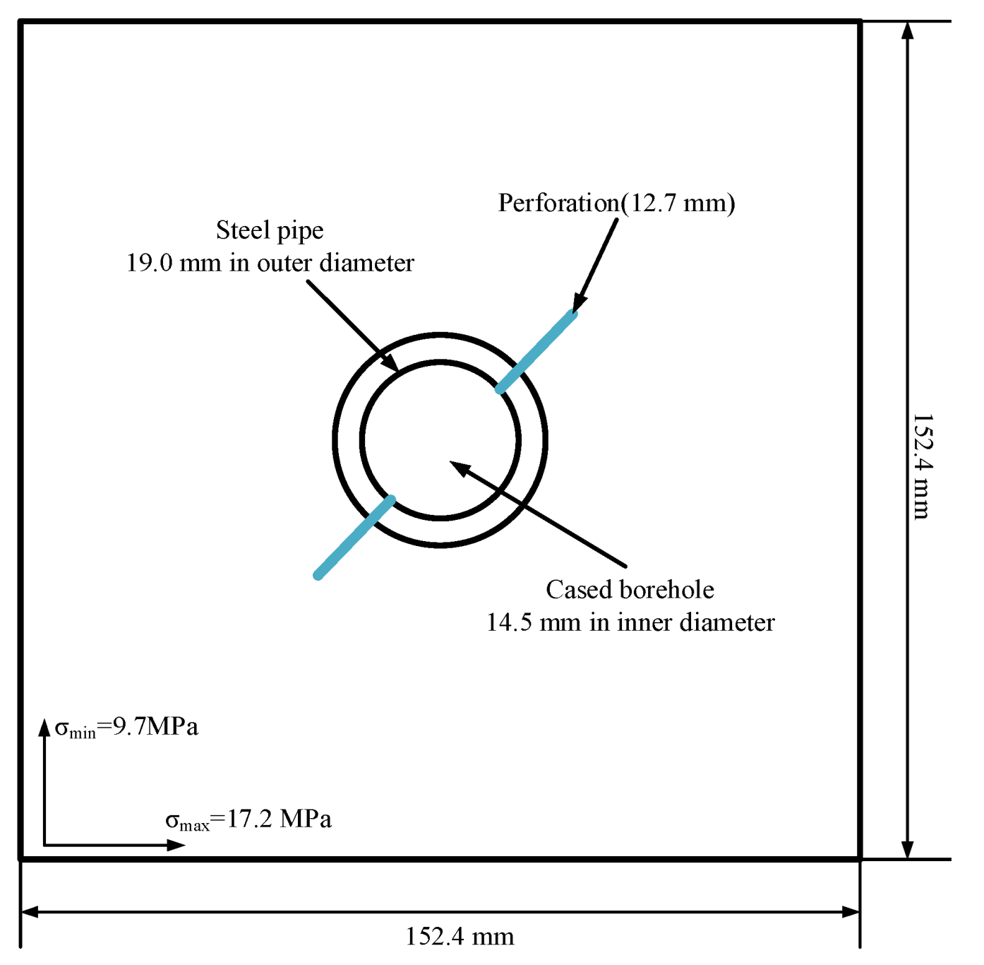
2.2. Model Validation Case 1: Abass’ Laboratory Experiments

2.2.1. Model Establishment and Micro-Property Calibration

Abass et al. [20,23] experimentally studied hydraulic fracturing at different perforation angles.

Table 1. Mechanical properties of hydrostone samples and experimental conditions in Abass et al.’s experiment [20,23].

Density (kg/m3)	Young’s Modulus (GPa)	Poisson’s Ratio	Internal Friction Angle (°)	Uniaxial Compressive Strength (MPa)	Tensile Strength (MPa)	Cohesion (MPa)	Fluid Viscosity (Pa·s)	Flow Rate (m³/s)
1710	14.3	0.21	45	55.4	5.6	11.5	1.18	5 × 10−7

shows the mechanical properties and injection parameters of hydrostone samples in the experiment. The T-W model is built according to the laboratory experiments of Abass et al. [20,23], and the geometry of the numerical samples is shown in Figure 1. The dimension of the 2D model is 152.4 mm (length) × 152.4 mm (width). The ring in the center of the model represents the steel pipe (outer diameter 19.0 mm, inner diameter 14.5 mm), and 2 perforations (with dimensions of 12.7 mm (in depth)) are created on the steel pipe at 180° phasing.

The model is divided into an assembly of Trigon blocks with an average side length of 2 mm, which is sufficiently small for rock materials [27,33]. The Trigon block is assumed to be elastic and does not fail. Its density, Poisson’s ratio and Young’s modulus are the same as those of the hydrostone sample, as shown in Table 1. The steel pipe is also assumed to be an elastomer and its density, Young’s modulus and Poisson’s ratio are 7500 Kg/m³, 160 GPa and 0.25, respectively [5]. The incipient fracture contact elements between the Trigon blocks follow the Coulomb slip model with residual strength, and both the residual tensile strength and residual cohesion are set to 0 [5]. It should be noted that the contact elements simulating the directional perforations are assigned with an extremely low friction angle, cohesion and tensile strength to ensure that these contact elements can fail at the beginning of fluid injection. Only mechanical boundary conditions are applied to the model boundaries. The maximum horizontal in-situ stress (σ_max) and the minimum horizontal in-situ stress (σ_min) are 17.2 MPa and 9.7 MPa, respectively [20,23]. The maximum allowable joint hydraulic aperture and the minimum allowable joint hydraulic aperture during fracturing are 6 × 10⁻³ m and 2 × 10⁻⁵ m, respectively [5]. The injection parameters are shown in Table 1.

In the UDEC model, densely packed blocks and contact elements are used to characterize the medium. Therefore, in addition to the mechanical properties of the Trigon blocks, the micro-properties of the contact elements should also be determined. In fact, the process of calibrating the micro-properties of the contact elements through the macro mechanical properties of hydrostone is a trial-and-error process, which follows the following procedures [27,34]: (1) adjust the shear stiffness and the normal stiffness of the contact elements until the Young’s modulus calculated by uniaxial compression test simulation matches the Young’s modulus of the rock according to the shear stiffness to normal stiffness ratio (k_s/k_n) equals the shear modulus to Young’s modulus ratio of the rock; (2) simulate the Brazilian tests with different contact tensile strengths until the simulation result matches the tensile strength of the rock; (3) adjust contact cohesion C_cont and contact friction angle φ_cont, and conduct a series of confined compression test simulations for each group of contact cohesion and contact friction angle. For each series of simulation results, the confining pressure-confined compressive strength curve can be fitted. The Y-axis intercept I and gradient G are then confirmed and used to calculate the cohesion C and friction angle φ of the rock by using Equations (5) and (6). This step is repeated until the matching cohesion C and friction angle φ are achieved.

$$\phi =arcsin\frac{g-1}{g+1}$$

(5)

$$C=i\frac{1-sin\phi }{2cos\phi }$$

(6)

During the calibration process, the model dimensions in the compression test simulation and the Brazilian test simulation are 50 mm (diameter) × 100 mm (height) and 50 mm (diameter), respectively. Each model is discretized into an assembly of Trigon blocks with an average side length of 2.5 mm [5,27,33]. All the Trigon blocks are assumed to be elastic, and their mechanical properties are shown in Table 1. According to the Coulomb slip criterion with residual strength, the contact element is regarded as an elastic-plastic body, and the residual strength is also set to 0 [5]. The loading velocities in the compression test simulation and the Brazilian test simulation are 0.1 m/s and 0.01 m/s, respectively [27]. Besides, the Young’s modulus is calculated from the more-or-less straight line in the stress–strain curve of the specimen under uniaxial compression and three confined compression test simulations are performed for each group of assumed contact cohesion C_cont and contact friction angle φ_cont, and the confining pressures are 0 MPa, 2.5 MPa and 5 MPa, respectively. This paper needs to calibrate the micro-properties of the contact elements when the homogeneity indexes are 2, 3 and 20, respectively.

Figure 2 shows the distributions of contact cohesion and contact tensile strength after calibration when the homogeneity indexes are 2 and 20, respectively.

Table 2. Mean micro-properties of hydrostone samples in UDEC T-W model after calibration under different homogeneity indexes (Properties of homogeneity index 2 is taken from reference [5]).

Homogeneity Index	Mean Shear Stiffness (GPa/m)	Mean Normal Stiffness (GPa/m)	Mean Contact Tensile Strength (MPa)	Mean Contact Cohesion (MPa)	Mean Contact Friction Angle (°)
2	590,000	1,416,000	40	82	70
3	300,000	720,000	22	58	55
20	236,000	571,120	10	31	34

provides the detailed calibration results. As can be seen from the calibration results, the mean values of micro-properties gradually decrease, and the distribution ranges of contact cohesion (Figure 2a,b) and contact tensile strength (Figure 2c,d) also gradually shrink (that is, the closer to the mean values) once the homogeneity index increases from 2 to 20.

Figure 3 shows the failure modes and total stress–strain curves of hydrostone samples in the confined compression test simulations (taking the confining pressure of 2.5 MPa as an example) and the failure modes and stress–displacement curves in the Brazilian test simulations. The results elucidate that mainly irregular shear failure dominates the failure pattern of the relatively heterogeneous hydrostone sample (m = 2) (Figure 3a). The sample shows the characteristics of plastic failure, which has already generated a large axial strain before reaching the peak stress and has a certain post-peak residual strength. However, the relatively homogeneous hydrostone sample is dominated by the brittle shear failure pattern on the diagonal (m = 20) (Figure 3b). The sample exhibits the characteristics of brittle failure and suddenly fails under relatively small axial strain, which is exactly consistent with the failure patterns of the confined compression test models obtained by the published UDEC Trigon modeling method [27]. Besides, the hydrostone specimen in the Brazilian test simulation has a more complex tensile failure plane and generates a larger axial displacement if the specimen is simulated at a lower homogeneity index (m = 2) (Figure 3c,d). Moreover, both the confined compression test model and the Brazilian test model have generated a large number of randomly distributed failure elements at the initial loading stage if the homogeneity index is 2 (Figure 3a,c).

In summary, variations in the homogeneity degree greatly affect the distributions of micro-properties (Figure 2), and thus influence the macroscopic and microscopic mechanical responses of the models (Figure 3). In the model with low homogeneity degrees, a slight disturbance will cause the failed contact elements. Before hydraulic fracturing, the heterogeneous model needs to be solved to an equilibrium state, which will result in generating randomly distributed failure contact elements that are the preferred pathways of HF propagation. This reveals the reason why HFs in heterogeneous rocks always propagate randomly and distribute asymmetrically when using the UDEC T-W method to simulate hydraulic fracturing.

2.2.2. Validation Results

The T-W model is adopted to reproduce the experiments of Abass et al. [20,23] at the perforation angles of 45°, 60°, 75° and 90°, assuming that the homogeneity index of laboratory-scale hydrostone samples is 3. The simulation results are shown in Figure 4. Figure 4a depicts the schematic diagram of HF re-orientation from artificial weaknesses. As can be seen from Figure 4b–g, the results of He et al. [5] (black line in the figure) are not quite consistent with the experimental results of Abass et al. [20,23]. The HF re-orientation distance of the experiment is overestimated at the perforation angle of 45°, while the experimental HF re-orientation distances are underestimated at the perforation angles of 60° and 75°. In contrast, the simulation results (red line in the figure) coincide with the experimental results when the homogeneity index is 3. In addition, the experiment at the perforation angle of 90° is also replicated, and the simulation results (red lines in Figure 4h,i) basically coincide with the experimental result. Obviously, the simulation results in this paper are more in line with the experimental results of Abass et al. [20,23], which improves the reliability of He et al. [5]’s validation results. The comparison of the simulation results when the homogeneity indexes are 3 and 2 indicates that rock heterogeneity is one of the important factors affecting the HF propagation trajectory, and the proper selection of the homogeneity index is the premise of simulation study.

It is worth noting that the validation only confirms the capability of the T-W model to accurately predict the HF re-orientation trajectory. The ability of the T-W model to predict other important hydraulic fracturing parameters (such as fracture width and breakdown pressure) needs to be verified in future studies.

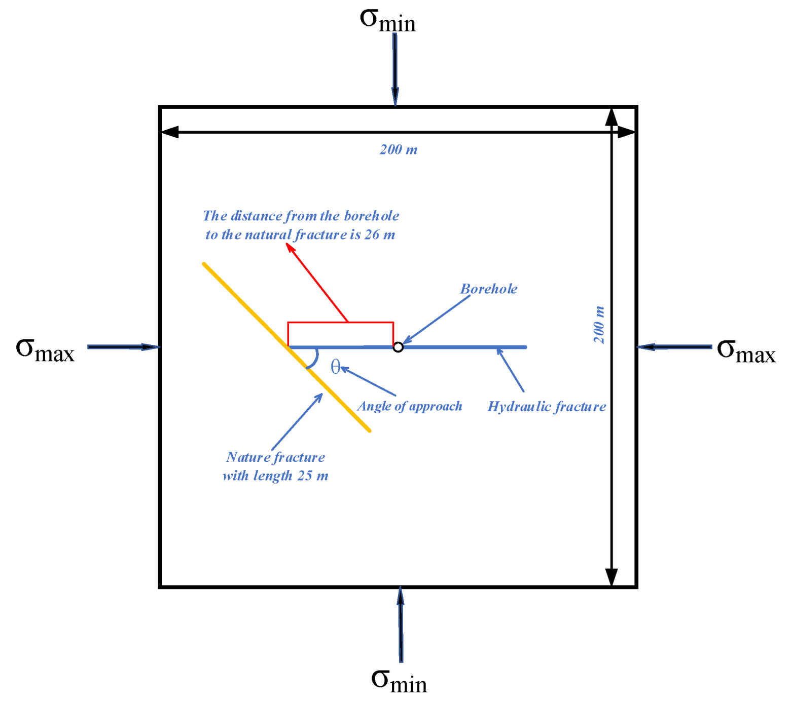
2.3. Model Validation Case 2: Zangeneh’s Numerical Simulations

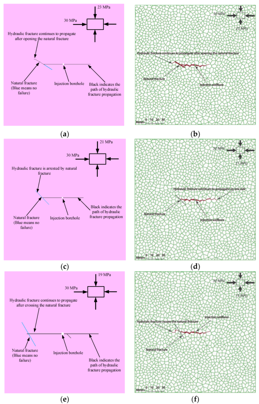
2.3.1. Effects of Natural Fracture on Hydraulic Fracturing

Affected by geological processes, underground rock masses usually include extensive natural fractures. Numerous studies suggest that HF propagation becomes complicated and unpredictable due to these pre-existing defects [12,35,36]. Zheng et al. [37] performed sensitivity analysis on factors affecting the interaction between HFs and NFs by using the hurricane analysis method, and believed that the approach angle and differential stress were the crucial factors. Zangeneh et al. [12] simulated the behavior of HFs when they encountered NFs under the conditions of different approach angles and differential stresses. The simulation results indicated three types of HF behavior: (1) NFs were opened and HFs could propagate along NFs at low differential stresses and low approach angles; (2) HFs tended to cross pre-existing NFs under high differential stresses and high approach angles; (3) HFs would be arrested by NFs when differential stresses and approach angles were intermediate.

Table 3. Typical cases under different approach angles and differential stresses in Zangeneh et al. [12].

Interaction Behavior	σmax (MPa)	σmin (MPa)	Differential Stress (MPa)	Angle of Approach (°)
Crossing	30	19	11	60
Offsetting	30	23	7	30
Arresting	30	21	9	45

clearly records three typical cases simulated by Zangeneh et al. [12]. In this paper, the T-W modeling method will be adopted to reproduce them to demonstrate that the T-W modeling method is able to simulate HF propagation in naturally fractured reservoirs.

2.3.2. Model Establishment and Validation Results

In this section, the numerical model of Zangeneh et al. [12] is rebuilt by the T-W modeling method. The geometry of the two-dimensional model sample is shown in Figure 5. The model dimension is 200 m (length) × 200 m (width). The Trigon logic is adopted here to generate incipient fractures as potential pathways for HF propagation. Besides, a joint with a length of 25 m is embedded as a natural fracture at a distance of 26 m from the left side of the borehole.

The model is discretized into a large number of Trigon blocks with an average side length of 4 m. All the Trigon blocks are modeled as being elastic, and their mechanical properties are derived from laboratory tests of reservoir rocks in northeastern British Columbia, as shown in

Table 4. Mechanical properties in Zangeneh et al.’s numerical simulation [38].

Internal Friction Angle (°)	Young’s Modulus (GPa)	Poisson’s Ratio	Cohesion (MPa)	Tensile Strength (MPa)	Uniaxial Compressive Strength (MPa)	Density (kg/m3)
30	30	0.25	15.6	4	53.9	2700

[38]. All the contact elements in the model follow the Coulomb slip criterion with residual strength, and the residual strength is set to 0 during the simulation [12].

Table 5. Mean micro-properties of incipient fractures after calibration under different homogeneity indexes and micro-properties of natural fracture in the UDEC T-W model.

Homogeneity Index of Incipient Fractures’ Micro-properties	Mean Shear Stiffness (GPa/m)	Mean Normal Stiffness (GPa/m)	Mean Contact Tensile Strength (MPa)	Mean Contact Cohesion (MPa)	Mean Contact Friction Angle (°)
2	1,080,000	2,700,000	15	75	50
20	800,000	2,000,000	6.5	36	33
100	550,000	1,375,000	6.2	30	31
Natural Fractures’ Micro-Properties	Mean Shear Stiffness (GPa/m)	Mean Normal Stiffness (GPa/m)	Mean Contact Tensile Strength (MPa)	Mean Contact Cohesion (MPa)	Mean Contact Friction Angle (°)
	0.1	1	0	0	25

shows the input parameters of NF, as well as the micro-properties of incipient fractures calibrated according to the mechanical properties in Table 4 when the homogeneity indexes are 2, 20 and 100. Mechanical boundary conditions (see Figure 5 and Table 3) and initial flow conditions (initial pore pressure is 10 MPa) are applied to the model. The borehole at the center of the model is pressurized with an incompressible slickwater fracturing fluid whose dynamic viscosity is 0.001 Pa·s [39]. In the simulation of Zangeneh et al. [12], the flow rate of fracturing fluid is unknown, so it is assumed to be 5 × 10⁻⁶ m³/s to simulate the quasi-static loading process [40]. It should be noted that the initial aperture value of incipient fractures is 0.01 mm, while that of NF is 0.1 mm. Variations in aperture follow a linear relationship described by the normal stiffness and normal displacement (see Table 5) [12].

Zangeneh et al. [12] explored the impact of approach angle and differential stress on the interaction between HFs and NFs in homogeneous rocks. Therefore, the homogeneity index of the T-W model is assumed to be 100 [32], and the three scenarios in Table 3 are validated. The simulation results are listed in Figure 6. When the approach angle is equal to 30°, 45° and 60°, the results obtained by the T-W modeling method are crossing (Figure 6a), offsetting (Figure 6c) and arresting (Figure 6e), respectively, which is consistent with the results of Zangeneh et al. [12]. The results illustrate that the T-W modelling method can simulate the interaction between HFs and NFs.

3. Analysis of Influencing Factors of HF Re-Orientation in Heterogeneous Rocks

3.1. Modelling Schemes

The validation result proves that the T-W modelling method is capable of simulating various scenarios of HF propagation in rocks of different homogeneity degrees on both laboratory scales and field scales. Based on the T-W modeling method, the following simulates the effects of fluid rate, fluid viscosity, perforation angle and NF on HF re-orientation from artificial weaknesses in heterogeneous rocks. All simulations run 3000 fluid steps to eliminate the effect of fracturing time on the HF propagation trajectory. Firstly, the influence of fluid velocity, fluid viscosity and perforation angle is researched by using the validated model of Abass et al. [20,23] when the homogeneity indexes are 2 and 20. Then, the numerical model of Zangeneh et al. [12] is fully utilized to analyze the impact of NF on HF re-orientation under the condition that the homogeneity indexes are 2 and 20.

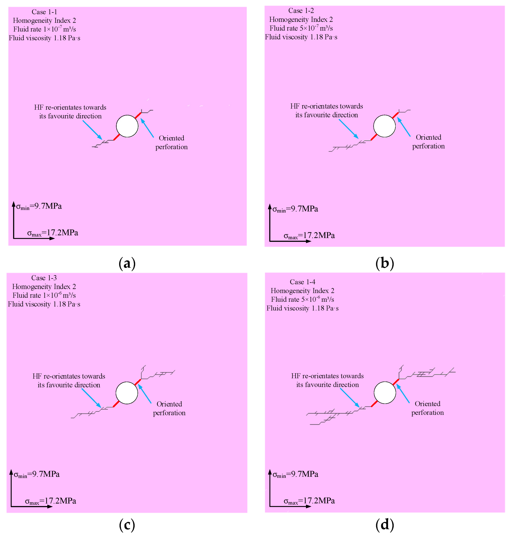
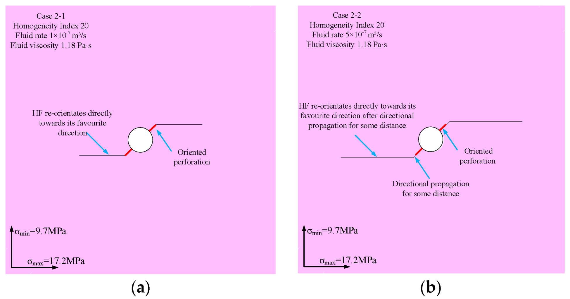
3.2. Effect of Fluid Rate

Table 6. Modelling scenarios to study the effect of fluid rate on HF re-orientation in heterogeneous rocks.

Modelling Scenarios	Modelling Cases	Fluid Rate (m³/s)	Fluid Viscosity (Pa·s)	Perforation Angle	Differential Stress (MPa)	Homogeneity Index
Scenario 1	Case 1–1	1 × 10−7	1.18	45°	7.5 MPa	2
	Case 1–2	5 × 10−7
	Case 1–3	1 × 10−6
	Case 1–4	5 × 10−6
Scenario 2	Case 2–1	1 × 10−7	1.18	45°	7.5 MPa	20
	Case 2–2	5 × 10−7
	Case 2–3	1 × 10−6
	Case 2–4	5 × 10−6

details the simulation scenarios to study the effect of flow rate on HF re-orientation. Figure 7 shows the HF re-orientation trajectories in scenario 1, where the homogeneity index is 2. From case 1–1 to case 1–4, the fluid rate increases from 1 × 10⁻⁷ m³/s to 5 × 10⁻⁶ m³/s, ensuring that hydraulic fracturing is always simulated in a quasi-static mode [40]. The results show that the HF re-orientation distance gradually increases and the final HF propagation trajectory becomes more complex with the increasing the fluid rate. Moreover, the HF propagates asymmetrically in the heterogeneous model (m = 2) and many fracture branches appear on the two wings of HFs at higher fluid rates (Figure 7c,d). Figure 8 provides the simulation results in scenario 2, in which the homogeneity index is 20. In the relatively homogeneous model, the HF presents symmetric two-wing propagation and its directional propagation distance along the perforation direction gradually increases with the increase of fluid rate. However, these HFs directly re-orientate towards the σ_max direction after certain directional propagation distances.

The results in Figure 7 and Figure 8 support that increasing the flow rate will enhance the guidance of perforations on HF propagation and promote HF propagation along the perforation direction, no matter if it is in heterogeneous rocks or relatively homogeneous rocks. However, the fluid rate determines the HF re-orientation trajectory in heterogeneous rocks, while the differential stress seems to be a more important factor in relatively homogeneous rocks and increasing the fluid rate will weaken the impact of differential stress.

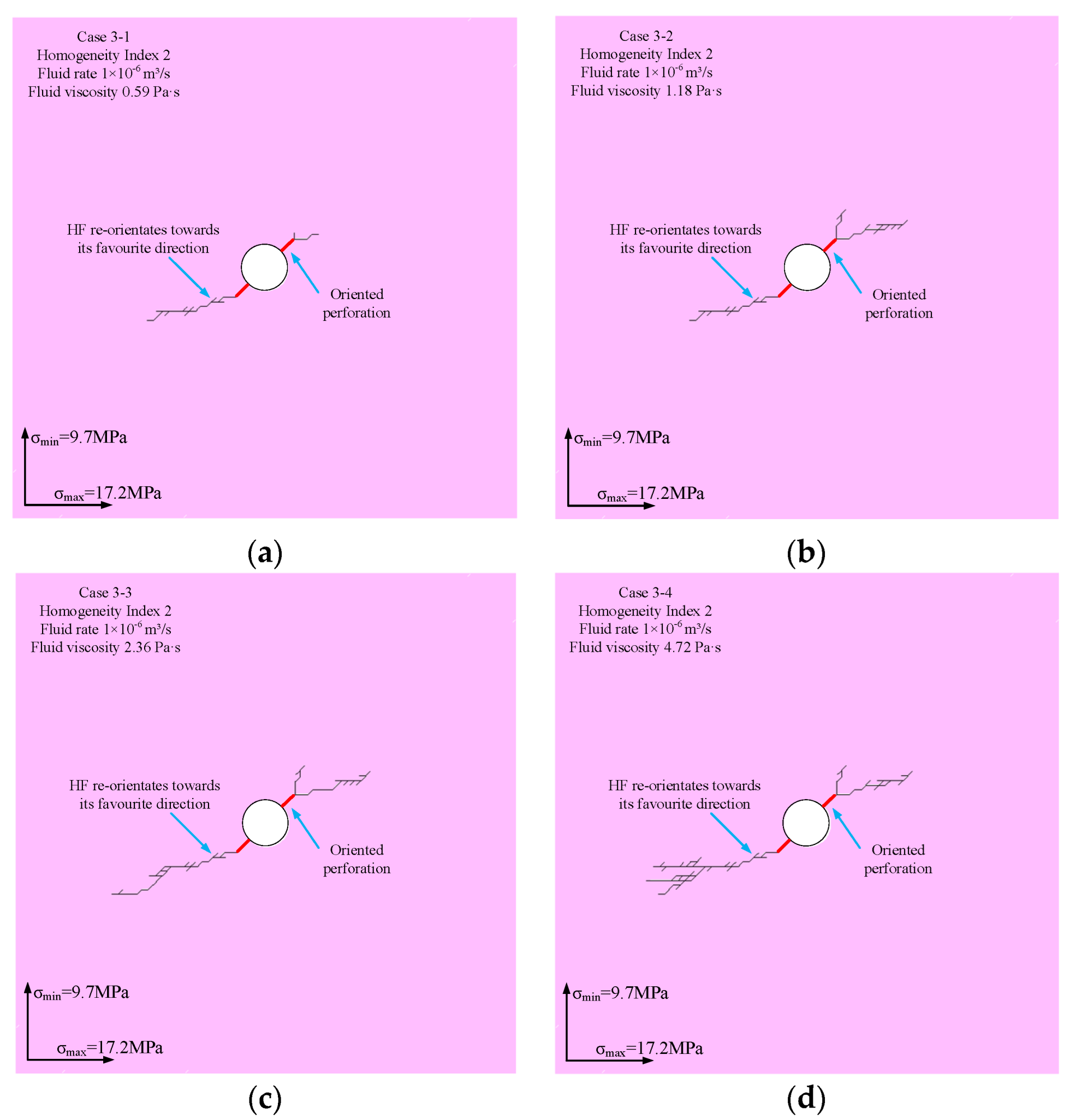
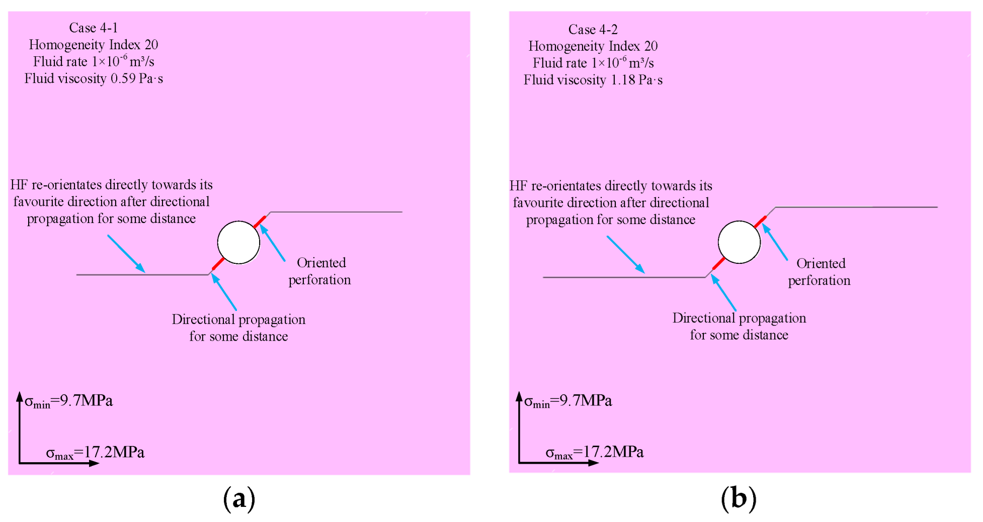
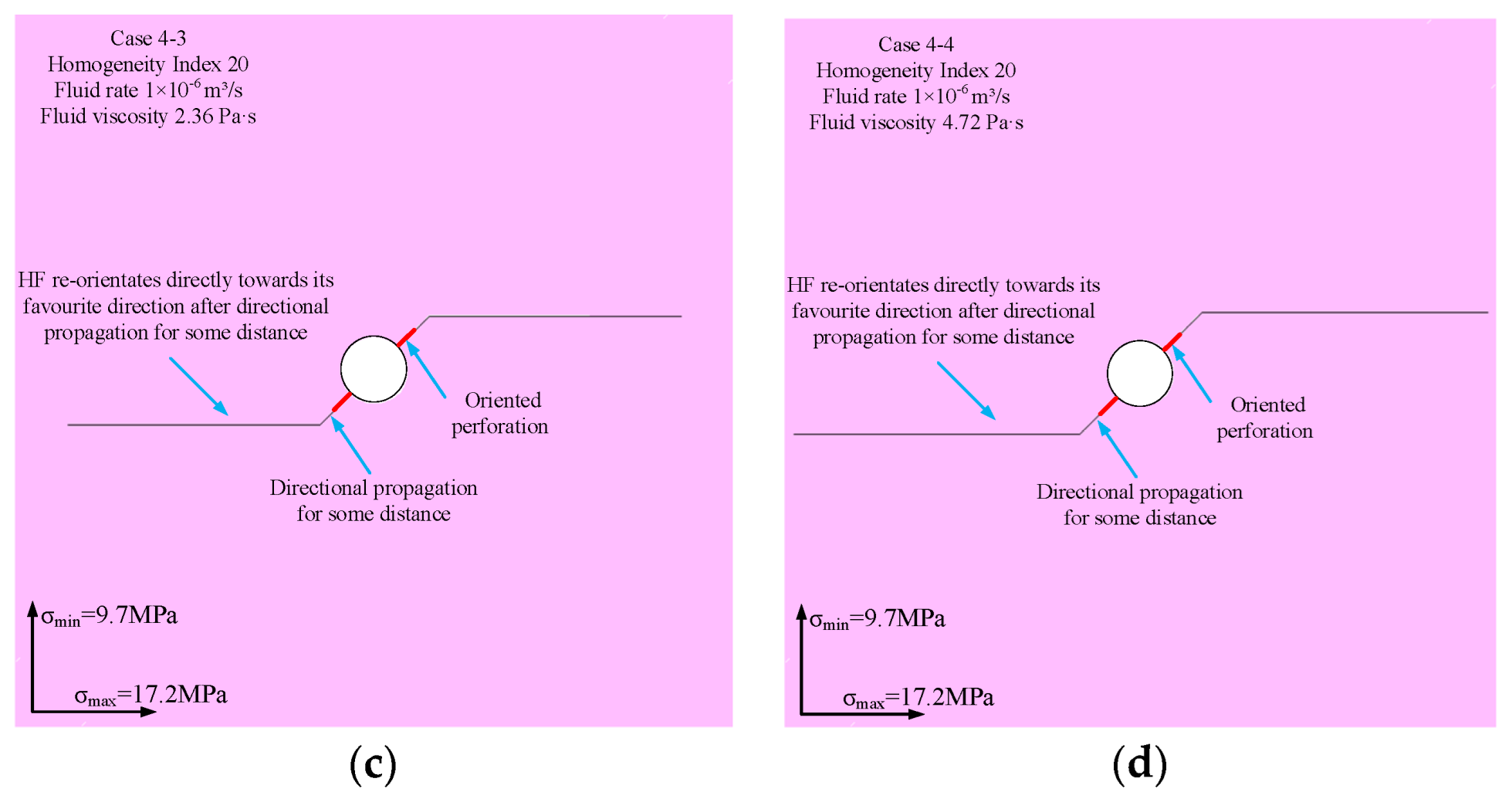
3.3. Effect of Fluid Viscosity

As can be seen from Section 3.2, only single-wing fractures will be generated in the heterogeneous rock specimens when fluid rates are lower than 1 × 10⁻⁶ m³/s (Figure 7a,b), while the HF will run through the relatively homogeneous rock specimen when the flow rate is higher than 1 × 10⁻⁶ m³/s (Figure 8d). Therefore, the fluid rate in this section is fixed at 1 × 10⁻⁶ m³/s to analyse the effect of fluid viscosity on HF re-orientation.

Table 7. Modelling scenarios to study the effect of fluid viscosity on HF re-orientation in heterogeneous rocks.

Modelling Scenarios	Modelling Cases	Fluid Rate (m³/s)	Fluid Viscosity (Pa·s)	Perforation Angle	Differential Stress (MPa)	Homogeneity Index
Scenario 3	Case 3–1	1 × 10−6	0.59	45°	7.5 MPa	2
	Case 3–2		1.18
	Case 3–3		2.36
	Case 3–4		4.72
Scenario 4	Case 4–1	1 × 10−6	0.59	45°	7.5 MPa	20
	Case 4–2		1.18
	Case 4–3		2.36
	Case 4–4		4.72

provides simulation scenarios for the study. Figure 9 and Figure 10 provide the HF propagation trajectories under different fluid viscosity when the homogeneity indexes are equal to 2 (scenario 3) and 20 (scenario 4), respectively. Obviously, the influence of fluid viscosity on HF re-orientation is similar to that of fluid rate: Whether in heterogeneous rocks or relatively homogeneous rocks, increasing fluid viscosity will improve the guided effect of perforations on HF paths and promote HF propagation along the perforation direction. However, the fluid viscosity dictates the HF re-orientation trajectory in heterogeneous rocks, whereas the differential stress seems to be a more significant factor in relatively homogeneous rocks and the impact of differential stress on HF re-orientation can be weakened by increasing fluid viscosity.

The findings reveal that the influence laws and principles of fluid viscosity on HF re-orientation are similar to those of fluid rate in both heterogeneous and relatively homogeneous rocks. The increase in flow rate or fluid viscosity gradually diminishes the lateral fluid leak-off, which significantly increases the volume of fluid flowing along the perforation direction, thereby enhancing the guidance of perforation on HF propagation and improving the fracturing performance. Besides, the HF propagation trajectory does not change when the fluid viscosity and fluid rate are changed within a reasonable range under the same homogeneity index and the constant product of fluid viscosity and fluid rate. (See Figure 7b and Figure 9a; Figure 7c and Figure 9b; Figure 8b and Figure 10a; Figure 8c and Figure 10b).

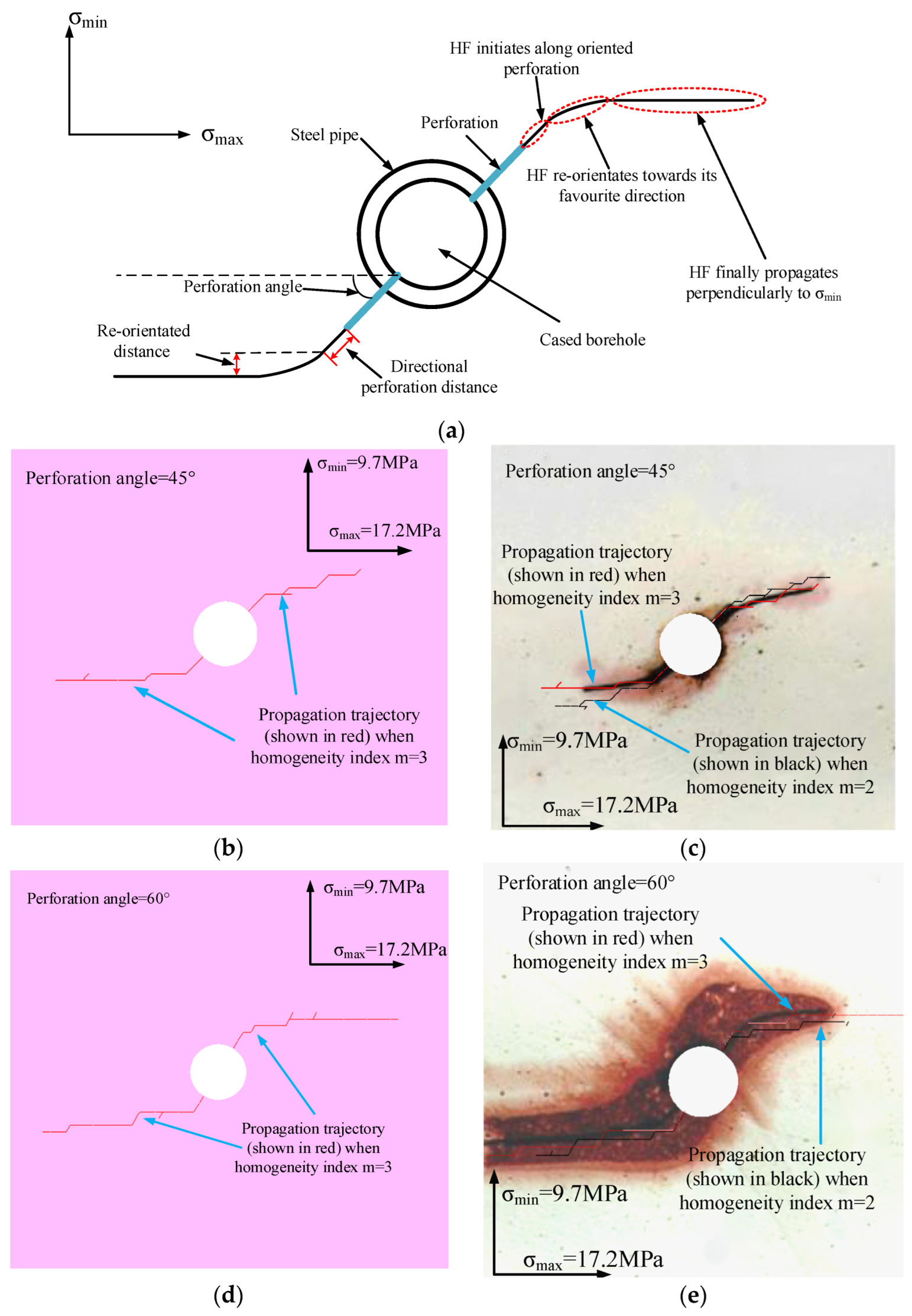
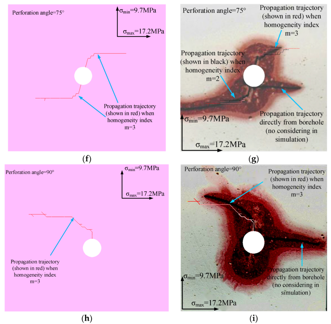
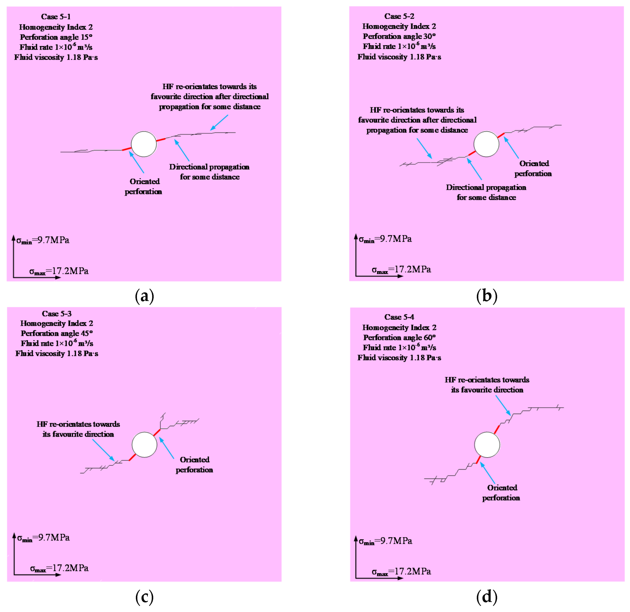
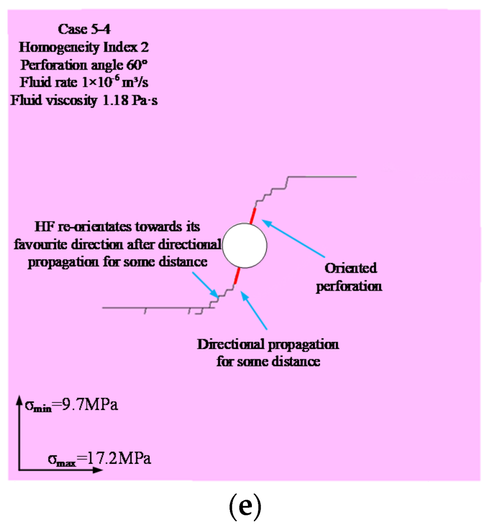
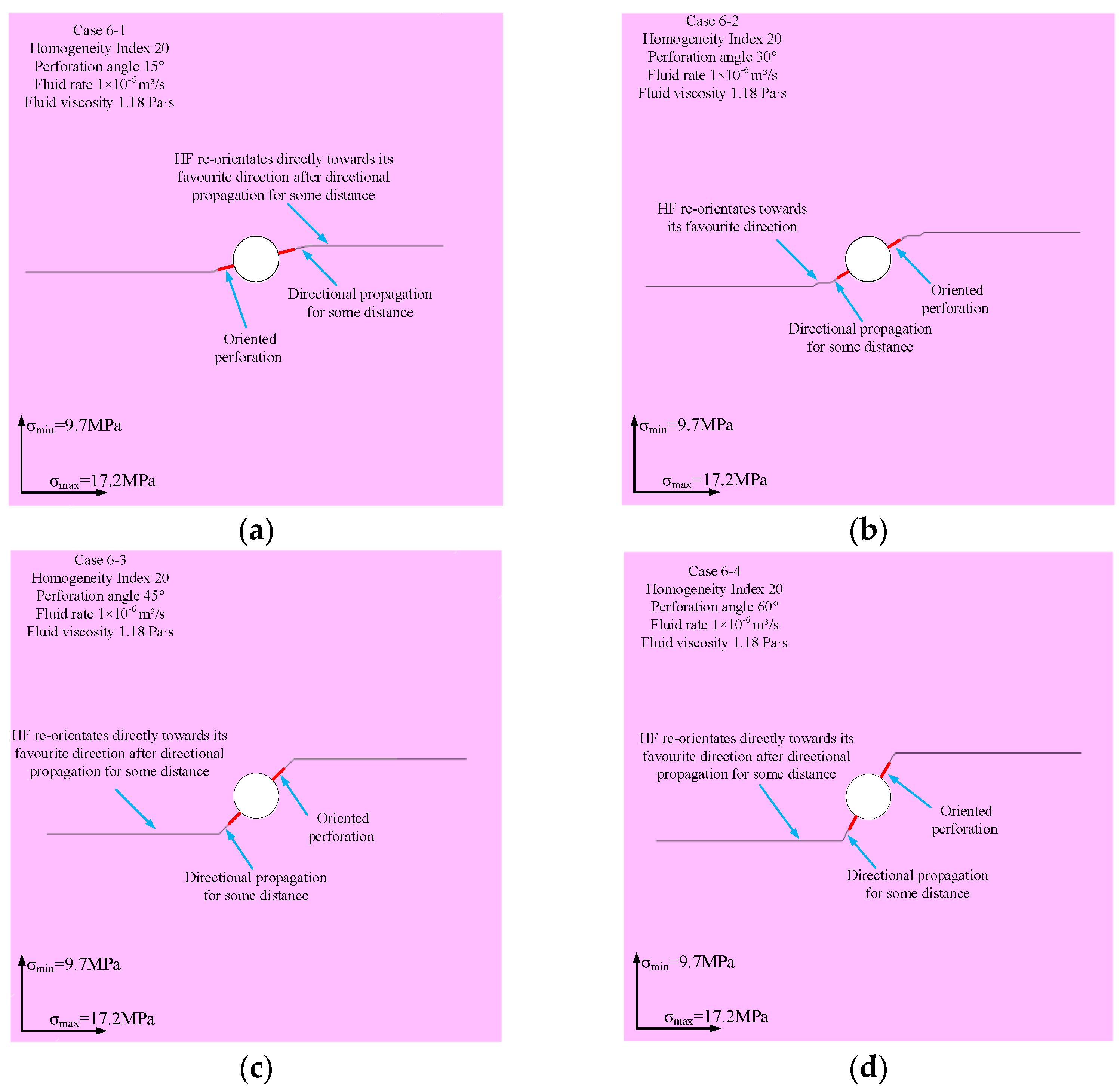
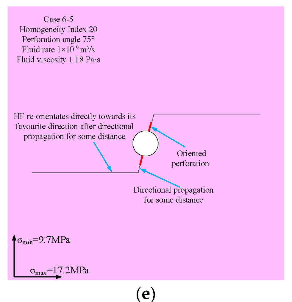
3.4. Effect of Perforation Angle

In this section, hydraulic fracturing at the perforation angles of 15°, 30°, 45°, 60° and 75° is simulated when the homogeneity indexes are 2 and 20, respectively. According to the simulation results in Section 3.2 and Section 3.3, the injection parameters here are 1 × 10⁻⁶ m³/s and 1.18 Pa·s.

Table 8. Modelling scenarios to study the effect of perforation angle on HF re-orientation in heterogeneous rocks.

Modelling Scenarios	Modelling Cases	Fluid Rate (m³/s)	Fluid Viscosity (Pa·s)	Perforation Angle	Differential Stress (MPa)	Homogeneity Index
Scenario 5	Case 5–1	1 × 10−6	1.18	15°	7.5 MPa	2
	Case 5–2			30°
	Case 5–3			45°
	Case 5–4			60°
	Case 5–5			75°
Scenario 6	Case 6–1	1 × 10−6	1.18	15°	7.5 MPa	20
	Case 6–2			30°
	Case 6–3			45°
	Case 6–4			60°
	Case 6–5			75°

provides the details of scenarios 5 and 6. Figure 11 and Figure 12 are the simulated results of these scenarios, respectively. Figure 11 illustrates that the re-orientation distance gradually increases by increasing the perforation angle in heterogeneous rocks (m = 2). It is worth noting that the perforation angle of 45° appears to be a critical angle. When perforation angles are less than 45°, the HF re-orientation distances are very short and HFs initiating from perforations rapidly re-orientate towards their favorite directions (Figure 11a,b), whereas HFs undergo obvious re-orientation processes and the re-orientation distance increases rapidly with the increase of perforation angle when perforation angles are greater than 45° (Figure 11c–e). Figure 12 lists the HF propagation trajectories of different perforation angles in relatively homogeneous rocks (m = 20). Obviously, the change of perforation angle has little influence on the HF re-orientation process in relatively homogeneous rocks. Although HFs undergo certain directional propagation distances, the distances are nearly equal. Therefore, this is more likely to be the cause of high fluid viscosity and fluid rate.

Figure 11 and Figure 12 suggest that the use of large perforation angles is efficient in guiding HF propagation within certain distances if the rock is relatively heterogeneous. However, the control of perforations over HF propagation might be limited in relatively homogeneous rocks. He et al. [5] believes that borehole arrangements under these circumstances should consider the direction of in-situ stress. The borehole axis should be aligned with the minimum in-situ stress direction if a series of radial HFs are required or perpendicular to the minimum in-situ stress direction if a series of axial HFs are expected. Other strategies are suggested, such as weakening the effect of differential stress by increasing the fluid rate or fluid viscosity to improve the guidance effect of perforation on HFs.

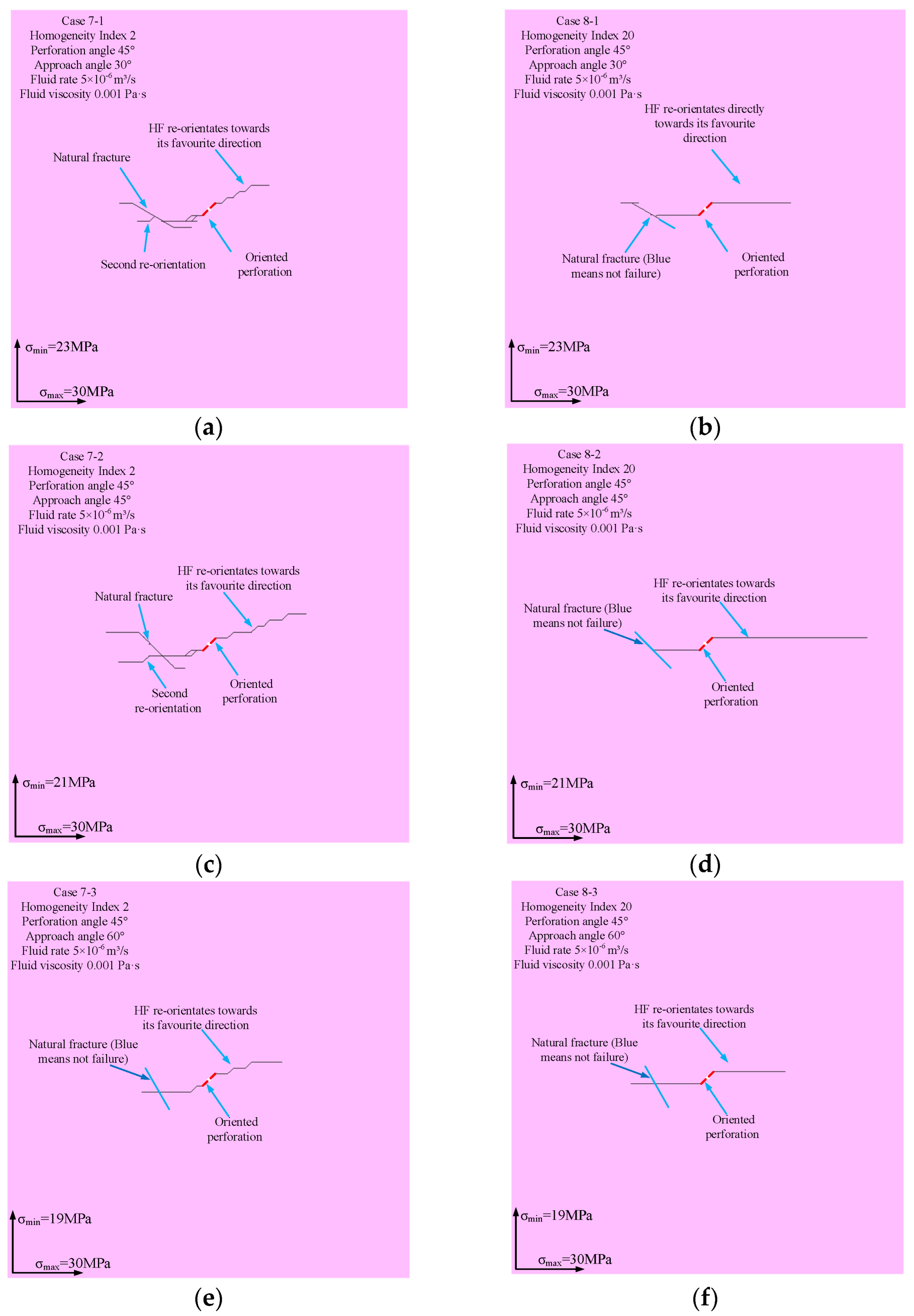
3.5. Effect of Natural Fracture

The T-W model is utilized to investigate the mechanical behavior of HFs after encountering NFs when the homogeneity indexes are 2 and 20, respectively, to analyse the influence of NF on HF re-orientation in heterogeneous rocks.

Table 9. Modelling scenarios to study the effect of NF on HF re-orientation in heterogeneous rocks.

Modelling Scenarios	Modelling Cases	Fluid Rate (m³/s)	Fluid Viscosity (Pa·s)	Perforation Angle	σmax (MPa)	σmin (MPa)	Approach Angle of NF	Homogeneity Index
Scenario 7	Case 7–1	5 × 10−6	0.001	45°	30	23	30°	2
	Case 7–2				30	21	45°
	Case 7–3				30	19	60°
Scenario 8	Case 8–1	5 × 10−6	0.001	45°	30	23	30°	20
	Case 8–2				30	21	45°
	Case 8–3				30	19	60°

gives the relevant parameter settings in simulation scenarios 7 and 8, in which the approach angles are 30°, 45° and 60° (which are consistent with the selection of Zangeneh et al. [12]), while the perforation angle is fixed at 45°. Figure 13 provides the simulation results of scenarios 7 and 8. The rock is relatively homogeneous (m = 20) in cases 8–1, 8–2, and 8–3 (Figure 13b,d,f). The results indicate that HFs propagate directly towards the σ_max direction once they initiate from perforations, and the mechanical behaviors of HFs after encountering NFs are no different from those in the previous study [12]. However, HFs first undergo certain re-orientation distances, and then exhibit unusual behaviors after encountering NFs in cases 7–1, 7–2, and 7–3 (m = 2) (Figure 13a,c,e). The NF is not only opened, but also induces secondary HF re-orientation in the middle of the NF when the approach angle is 30° (Figure 13a). Besides, when the approaching angle is 45°, the HF is not arrested. On the contrary, the NF is opened and the HF reorientates again in the middle and the tip of the NF (Figure 13c). The above phenomena may be caused by the low micro-properties of the contact elements at the point where HFs encounter NFs in heterogeneous rocks.

The findings support that rock heterogeneity significantly influences the mechanical behavior of HFs after encountering NFs. In heterogeneous rocks, HFs initiating from artificial weaknesses will have secondary re-orientation if HFs can open NFs and propagate along them (Figure 13a,c), which is equivalent to increasing the HF re-orientation distance.

4. Discussion

The heterogeneity of rock micro-properties affect the reliability of hydraulic fracturing numerical simulations, and selecting a reasonable method to represent heterogeneous rocks is the premise of numerical simulations (Figure 4b–g). In this paper, the Weibull distribution is adopted to reasonably represent the micro-properties of heterogeneous rocks, so as to obtain the complex and asymmetric HF propagation trajectories (Figure 7, Figure 9 and Figure 11), which are closer to the HF geometry detected in field applications by micro-seismic waves [41].

The findings (Section 3.2, Section 3.3, Section 3.4 and Section 3.5) in this paper show that the degree of rock heterogeneity needs to be determined first, which is helpful to select reasonable construction conditions. For example, in heterogeneous rocks, the HF propagation paths are more likely to be controlled by directional perforations, large perforation angles and high injection parameters highlight this effect (Figure 7, Figure 9 and Figure 11). In homogeneous rocks, however, the change of perforation angle does not have an impact on HF re-orientation (Figure 12). On the contrary, the differential stress and injection parameters are more able to direct the propagation path of hydraulic fracturing. The high fluid viscosity or high fluid rate is recommended to improve the effect of perforation on guiding the HF propagation paths (Figure 8 and Figure 10). Moreover, the effect of differential stress can be attenuated by modulating the relative direction between the borehole axis and the minimum in-situ stress in relatively homogeneous rocks.

On the other hand, NFs are another important factor influencing the HF re-orientation trajectories. NFs that are opened can induce secondary HF re-orientation in heterogeneous rocks (Figure 13a,c), which needs to be considered when designing hydraulic fracturing using artificial weaknesses.

5. Conclusions

Many factors affect HF re-orientation from artificial weaknesses, including rock heterogeneity, injection parameters, perforation angle and NF, which have either synergetic or competitive effects under different circumstances. Based on the UDEC T-W modeling method, the effects of fluid viscosity, fluid rate, perforation angle and NF on HF re-orientation from artificial weaknesses in heterogeneous rocks are studied. The main conclusions are as follows:

(1)

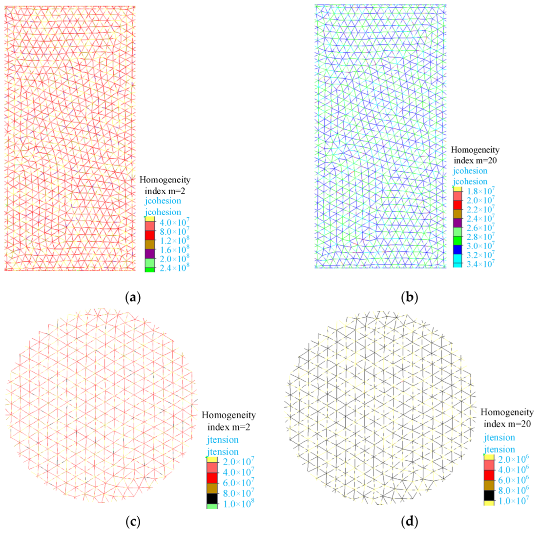
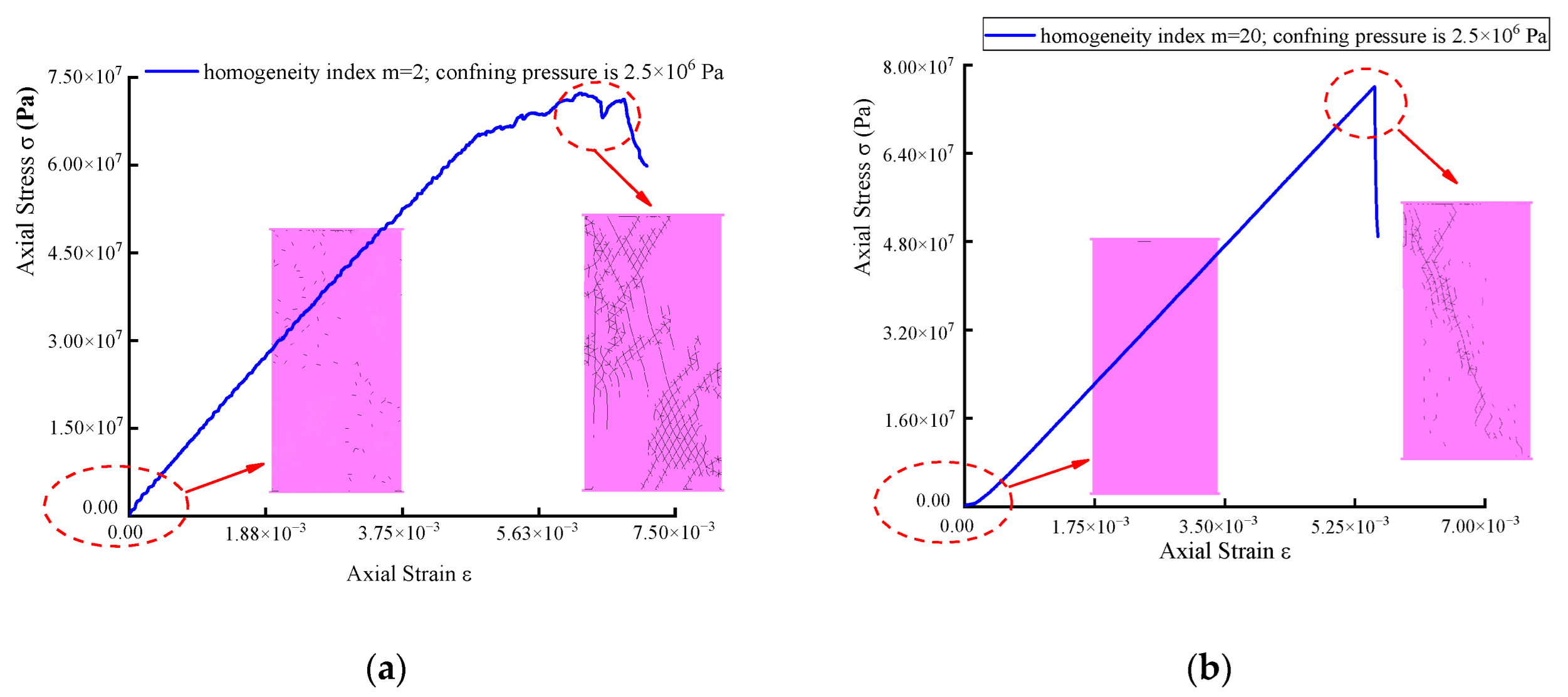
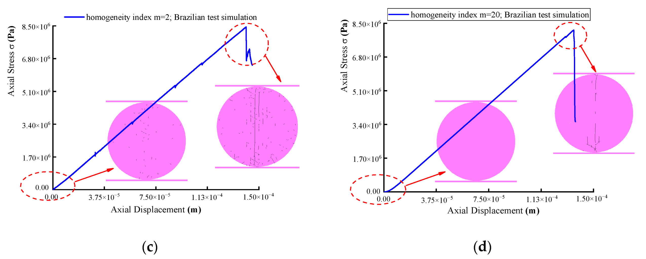
Variations in rock heterogeneity greatly affect the distributions of contact micro-properties (Figure 2), and thus influence the macroscopic and microscopic mechanical responses of the models (Figure 3). Generally, a slight disturbance will cause the failed contact elements in the model with low homogeneity degrees, which will result in generating randomly distributed failure contact elements that are the preferred pathways of HF propagation. This reveals the reason why HFs in heterogeneous rocks always propagate randomly and distribute asymmetrically when using the T-W method.

(2)

The Weibull distribution measures the homogeneity degree of rocks by means of the homogeneity index m, and the proper selection of homogeneity index is the premise of researches. The simulation results with the homogeneity index of 3 are closer to the experimental results than those with the homogeneity index of 2 when taking advantage of the experiments of Abass et al. [20,23] to validate the T-W modeling method. Moreover, by reproducing the numerical simulation of Zangeneh et al. [12], the T-W modeling method is also applicable to simulate the influence of rock heterogeneity on hydraulic fracture re-orientation in naturally fractured reservoirs.

(3)

The rock heterogeneity affects the effects of fluid rate, fluid viscosity and perforation angle on HF re-orientation from artificial weaknesses. The HF re-orientation distance increases obviously and the guidance of perforation on HF propagation is enhanced with the increase of fluid rate, fluid viscosity and perforation angle in heterogeneous rocks. In contrast, the differential stress is the dominant influencing factor in relatively homogeneous rocks, causing HFs to rapidly re-orientate from the artificial weakness towards the theoretical prediction. However, increasing the fluid viscosity and fluid rate can weaken the impact of differential stress.

(4)

Natural fractures are another factor influencing the HF re-orientation trajectory. In heterogeneous rocks, NFs opened by HFs will induce secondary HF re-orientation.

References

1. Clark, J. A hydraulic process for increasing the productivity of wells. J. Pet. Technol. 1949, 1, 1–8. [Google Scholar] [CrossRef]
2. He, Q.Y.; Suorineni, F.T.; Oh, J. Modeling interaction between natural fractures and hydraulic fractures in block cave mining. In Proceedings of the 49th US rock Mechanics/Geomechanics Symposium, San Francisco, CA, USA, 29 June 2015. [Google Scholar]
3. Dunlop, E.C.; Salmachi, A.; McCabe, P.J. Investigation of increasing hydraulic fracture conductivity within producing ultra-deep coal seams using time-lapse rate transient analysis: A long-term pilot experiment in the Cooper Basin, Australia. Int. J. Coal Geol. 2020, 220, 103363. [Google Scholar] [CrossRef]
4. Cipolla, C.L.; Warpinski, N.R.; Mayerhofer, M.J. Hydraulic Fracture Complexity: Diagnosis, Remediation and Exploitation. In Proceedings of the SPE Asia Pacific Oil and Gas Conference and Exhibition, Perth, Australia, 20–22 October 2008. [Google Scholar]
5. He, Q.Y.; Zhu, L.; Li, Y.C.; Li, D.Q.; Zhang, B.Y. Simulating Hydraulic Fracture Re-orientation in Heterogeneous Rocks with an Improved Discrete Element Method. Rock Mech. Rock Eng. 2021, 54, 2859–2879. [Google Scholar] [CrossRef]
6. Lin, J.; Xu, C.; Yang, J. Study on the influence of pump flow rate on the deflection of hydraulic fracturing cracks in longitudinal flume cutting. J. Chin. Coal Soc. 2020, 45, 2804–2812. [Google Scholar]
7. He, Q.Y.; Suorineni, F.T.; Oh, J. Review of hydraulic fracturing for preconditioning in cave mining. Rock Mech. Rock Eng. 2016, 49, 4893–4910. [Google Scholar] [CrossRef]
8. He, Q.Y.; Suorineni, F.T.; Oh, J. Strategies for creating prescribed hydraulic fractures in cave mining. Rock Mech. Rock Eng. 2017, 50, 967–993. [Google Scholar] [CrossRef]
9. Hubbert, M.K.; Willis, D.G. Mechanics of hydraulic fracturing. Trans. AIME 1957, 210, 153–168. [Google Scholar] [CrossRef]
10. Daneshy, A.A. Hydraulic fracture propagation in the presence of planes of weakness. In Proceedings of the SPE-European Spring Meeting 1974 of the Society of Petroleum Engineers of AIME, Amsterdam, The Netherlands, 29–30 May 1974. [Google Scholar]
11. Behnia, M.; Goshtasbi, K.; Marji, M.F.; Golshani, A. Numerical simulation of interaction between hydraulic and natural fractures in discontinuous media. Acta Geotech. 2015, 10, 533–546. [Google Scholar] [CrossRef]
12. Zangeneh, N.; Eberhardt, E.; Bustin, R.M. Investigation of the influence of natural fractures and in situ stress on hydraulic fracture propagation using a distinct-element approach. Can. Geotech. J. 2015, 52, 926–946. [Google Scholar] [CrossRef] [Green Version]
13. Huang, L.K.; Liu, J.J.; Zhang, F.S.; Dontsov, E.; Damjanac, B. Exploring the influence of rock inherent heterogeneity and grain size on hydraulic fracturing using discrete element modeling. Int. J. Solids Struct. 2019, 176, 207–220. [Google Scholar] [CrossRef]
14. He, F.F.; Zhang, R.X.; Kang, T.H.; Kang, J.T.; Guo, J.Q. Dynamic propagation model for oriented perforation steering fracturing cracks in low permeability reservoirs based on microelement method. Chin. J. Rock Mech. Eng. 2020, 39, 782–792. [Google Scholar]
15. Huang, B.X.; Yu, B.; Feng, F.; Li, Z.; Wang, Y.Z.; Liu, J.R. Field investigation into directional hydraulic fracturing for hard roof in Tashan Coal Mine. J. Coal Sci. Eng. 2013, 19, 153–159. [Google Scholar] [CrossRef]
16. Behrmann, L.A.; Elbel, J.L. Effect of Perforations on Fracture Initiation. J. Pet. Technol. 1991, 43, 608–615. [Google Scholar] [CrossRef]
17. Jefrey, R.G.; Chen, Z.R.; Zhang, X.; Bunger, A.P.; Mills, K.W. Measurement and analysis of full-scale hydraulic fracture initiation and reorientation. Rock Mech Rock Eng. 2015, 48, 2497–2512. [Google Scholar] [CrossRef]
18. Vahab, M.; Akhondzadeh, S.; Khoei, A.R.; Khalil, A. An X-FEM investigation of hydro-fracture evolution in naturally-layered domains. Eng. Fract. Mech. 2018, 191, 187–204. [Google Scholar] [CrossRef]
19. Lekontsev, Y.M.; Sazhin, P.V. Directional hydraulic fracturing in difficult caving roof control and coal degassing. J. Min. Sci. 2014, 50, 914–917. [Google Scholar] [CrossRef]
20. Abass, H.H.; Meadows, D.L.; Brumley, J.L.; Hedayati, S.; Venditto, J.J. Oriented perforations-a rock mechanics view. In Proceedings of the SPE Annual Technical Conference and Exhibition, New Orleans, LA, USA, 24 September 1994. [Google Scholar]
21. Jefrey, R.; Mills, K. Hydraulic fracturing applied to inducing longwall coal mine goaf falls. In Proceedings of the 4th North American Rock Mechanics Symposium, Seattle, WA, USA, 31 July–3 August 2000. [Google Scholar]
22. Elbel, J.L.; Mack, M.G. Re-fracturing: Observations and theories. In Proceedings of the SPE Production Operations Symposium, Oklahoma City, OK, USA, 21–23 May 1993. [Google Scholar]
23. Abass, H.H.; Hedayati, S.; Meadows, D. Nonplanar fracture propagation from a horizontal wellbore: Experimental study. SPE Prod. Facil. 1996, 11, 133–137. [Google Scholar] [CrossRef]
24. Sesetty, V.; Ghassemi, A. A numerical study of sequential and simultaneous hydraulic fracturing in single and multi-lateral horizontal wells. J. Pet. Sci. Eng. 2015, 132, 65–76. [Google Scholar] [CrossRef]
25. He, Q.Y.; Suorineni, F.T.; Ma, T.; Oh, J. Parametric study and dimensional analysis on prescribed hydraulic fractures in cave mining. Tunn. Undergr. Space Technol. 2018, 78, 47–63. [Google Scholar] [CrossRef]
26. Weibull, W. A statistical distribution function of wide applicability. J. Appl. Mech. 1951, 18, 293–297. [Google Scholar] [CrossRef]
27. Gao, F.Q.; Stead, D. The application of a modified Voronoi logic to brittle fracture modelling at the laboratory and field scale. Int. J. Rock Mech. Min. Sci. 2014, 68, 1–14. [Google Scholar] [CrossRef]
28. Chen, W.; Konietzky, H.; Liu, C.; Tan, X. Hydraulic fracturing simulation for heterogeneous granite by discrete element method. Comput Geotech. 2018, 95, 1–15. [Google Scholar] [CrossRef]
29. Chen, S.; Yue, Z.Q.; Tham, L.G. Digital image-based numerical modeling method for prediction of inhomogeneous rock failure. Int. J. Rock Mech. Min. Sci. 2004, 41, 939–957. [Google Scholar] [CrossRef]
30. Fenton, G.A.; Griffifiths, D.V. Risk Assessment in Geotechnical Engineering; Wiley: Hoboken, NJ, USA, 2008. [Google Scholar]
31. Yang, T.H.; Tham, L.G.; Tang, C.A.; Liang, Z.Z.; Tsui, Y. Infuence of heterogeneity of mechanical properties on hydraulic fracturing in permeable rocks. Rock Mech. Rock Eng. 2004, 37, 251–275. [Google Scholar] [CrossRef]
32. He, Q.Y.; Suorineni, F.T.; Ma, T.; Oh, J. Effect of Discontinuity Stress Shadows on Hydraulic Fracture Re-orientation. Int. J. Rock Mech. Min. Sci. 2017, 91, 179–194. [Google Scholar] [CrossRef]
33. Kazerani, T.; Zhao, J. Micromechanical parameters in bonded particle method for modelling of brittle material failure. Int. J. Numer. Anal. Meth. Geomech. 2010, 34, 1877–1895. [Google Scholar] [CrossRef]
34. Zhang, S.; Xu, J.H.; Chen, L.; Shimada, H.; Zhang, M.W.; He, H.H. The Effects of Precrack Angle on the Strength and Failure Characteristics of Sandstone under Uniaxial Compression. Geofluids 2021, 2021, 7153015. [Google Scholar] [CrossRef]
35. Blanton, T.L. An experimental study of interaction between hydraulically induced and pre-existing fractures. In Proceedings of the SPE/DOE Unconventional Gas Recovery Symposium of the Society of Petroleum Engineers, Pittsburgh, PA, USA, 16–18 May 1982. [Google Scholar]
36. Dusseault, M.B.; McLennan, J.; Shu, J. Massive multi-stage hydraulic fracturing for oil and gas recovery from low mobility reservoirs in China. Petrol. Drill. Tech. 2011, 39, 6–16. [Google Scholar]
37. Kolawole, O.; Ispas, I. Interaction between hydraulic fractures and natural fractures: Current status and prospective directions. J. Petrol. Explor. Prod. Technol. 2020, 10, 1613–1634. [Google Scholar] [CrossRef] [Green Version]
38. McLellan, P.J.; Cormier, K. Borehole Instability in Fissile, Dipping Shales, Northeastern British Columbia. In Proceedings of the SPE Gas Technology Symposium, Calgary, AB, Canada, 28 April 1996. [Google Scholar]
39. Lecampion, B.; Zia, H. Slickwater hydraulic fracture propagation: Near-tip and radial geometry solutions. J. Fluid Mech. 2019, 880, 514–550. [Google Scholar] [CrossRef]
40. Zhao, X.Y.; Wang, T.; Elsworth, D.; He, Y.L.; Zhou, W.; Zhuang, L.; Zeng, J.; Wang, S.F. Controls of natural fractures on the texture of hydraulic fractures in rock. J. Petrol. Sci. Eng. 2018, 165, 616–626. [Google Scholar] [CrossRef]
41. Vermylen, J.; Zoback, M.D. Hydraulic fracturing, microseismic magnitudes, and stress evolution in the Barnett Shale. In Proceedings of the SPE Hydraulic Fracturing Technology Conference, The Woodlands, TX, USA, 24 January 2011. [Google Scholar]
Figure 1. Model schematic diagram of validation case 1 [5].
Machines 10 00152 g001
Figure 2. Contact cohesion and contact tensile strength distributions after calibration: (a) contact cohesion distributions under the confining pressure of 2.5 × 10⁶ Pa when the homogeneity index is 2; (b) contact cohesion distributions under the confining pressure of 2.5 × 10⁶ Pa when the homogeneity index is 20; (c) contact tension strength distributions under the Brazilian test simulation when the homogeneity index is 2; (d) contact tension strength distributions under the Brazilian test simulation when the homogeneity index is 20.
Machines 10 00152 g002
Figure 3. Monitoring curves and model failure modes: (a) full stress−strain curve and failure mode of the confined compression test simulation under the confining pressure of 2.5 × 10⁶ Pa when the homogeneity index is 2; (b) full stress−strain curve and failure mode of the confined compression test simulation under the confining pressure of 2.5 × 10⁶ Pa when the homogeneity index is 20; (c) displacement−stress curve and failure mode of the Brazilian test simulation when the homogeneity index is 2; (d) displacement−stress curve and failure mode of the Brazilian test simulation when the homogeneity index is 20.
Machines 10 00152 g003aMachines 10 00152 g003b
Figure 4. Validation results and comparison: (a) schematic of HF re-orientation; (b) the simulation result at a perforation angle of 45° when the homogeneity index is 3; (c) the simulation result (red line) when the homogeneity index is 3 is compared with the simulation result (black line) of He et al. [5] and the experimental result of Abass et al. [20,23] (perforation angle = 45°); (d) the simulation result at a perforation angle of 60° when the homogeneity index is 3; (e) the simulation result (red line) when the homogeneity index is 3 is compared with the simulation result (black line) of He et al. [5] and the experimental result of Abass et al. [20,23] (perforation angle = 60°); (f) the simulation result at a perforation angle of 75° when the homogeneity index is 3; (g) the simulation result (red line) when the homogeneity index is 3 is compared with the simulation result (black line) of He et al. [5] and the experimental result of Abass et al. [20,23] (perforation angle = 75°); (h) the simulation result at a perforation angle of 90° when the homogeneity index is 3; (i) the simulation result (red line) when the homogeneity index is 3 is compared with the experimental result of Abass et al. [20,23] (perforation angle = 90°).
Machines 10 00152 g004aMachines 10 00152 g004b
Figure 5. Model schematic diagram of validation case 2 [12].
Machines 10 00152 g005
Figure 6. The comparison between simulation results of T-W modeling method (m = 100) and the simulation records of Zangeneh et al. [12]: (a) T-W modeling method simulation result at the approach angle of 30° when the differential stress is 7 MPa; (b) simulation result of Zangeneh et al. [12] at the approach angle of 30° when the differential stress is 7 MPa; (c) T-W modeling method simulation result at the approach angle of 45° when the differential stress is 9 MPa; (d) simulation result of Zangeneh et al. [12] at the approach angle of 45° when the differential stress is 9 MPa; (e) T-W modeling method simulation result at the approach angle of 60° when the differential stress is 11 MPa; (f) simulation result of Zangeneh et al. [12] at the approach angle of 60° when the differential stress is 11 MPa.
Machines 10 00152 g006
Figure 7. The relationship between HF re-orientation and fluid rate when the homogeneity index is equal to 2: (a) fluid rate is 1 × 10⁻⁷ m³/s; (b) fluid rate is 5 × 10⁻⁷ m³/s; (c) fluid rate is 1 × 10⁻⁶ m³/s; (d) fluid rate is 5 × 10⁻⁶ m³/s.
Machines 10 00152 g007
Figure 8. The relationship between HF re-orientation and fluid rate when the homogeneity index is equal to 20: (a) fluid rate is 1 × 10⁻⁷ m³/s; (b) fluid rate is 5 × 10⁻⁷ m³/s; (c) fluid rate is 1 × 10⁻⁶ m³/s; (d) fluid rate is 5 × 10⁻⁶ m³/s.
Machines 10 00152 g008aMachines 10 00152 g008b
Figure 9. The relationship between HF re-orientation and fluid viscosity when the homogeneity index is equal to 2: (a) fluid viscosity is 0.59 Pa·s; (b) fluid viscosity is 1.18 Pa·s; (c) fluid viscosity is 2.36 Pa·s; (d) fluid viscosity is 4.72 Pa·s.
Machines 10 00152 g009
Figure 10. The relationship between HF re-orientation and fluid viscosity when the homogeneity index is equal to 20: (a) fluid viscosity is 0.59 Pa·s; (b) fluid viscosity is 1.18 Pa·s; (c) fluid viscosity is 2.36 Pa·s; (d) fluid viscosity is 4.72 Pa·s.
Machines 10 00152 g010aMachines 10 00152 g010b
Figure 11. The relationship between HF re-orientation and perforation angle when the homogeneity index is 2: (a) perforation angle is 15°; (b) perforation angle is 30°; (c) perforation angle is 45°; (d) perforation angle is 60°; (e) perforation angle is 75°.
Machines 10 00152 g011aMachines 10 00152 g011b
Figure 12. The relationship between HF re-orientation and perforation angle when the homogeneity index is 20: (a) perforation angle is 15°; (b) perforation angle is 30°; (c) perforation angle is 45°; (d) perforation angle is 60°; (e) perforation angle is 75°.
Machines 10 00152 g012aMachines 10 00152 g012b
Figure 13. The relationship between HF re-orientation and NFs: (a) the approach angle is 30°, the differential stress is 7 MPa and the homogeneity index is 2; (b) the approach angle is 30°, the differential stress is 7 MPa and the homogeneity index is 20; (c) the approach angle is 45°, the differential stress is 9 MPa and the homogeneity index is 2; (d) the approach angle is 45°, the differential stress is 9 MPa and the homogeneity index is 20; (e) the approach angle is 60°, the differential stress is 11 MPa and the homogeneity index is 2; (f) the approach angle is 60°, the differential stress is 11 MPa and the homogeneity index is 20.
Machines 10 00152 g013