Article

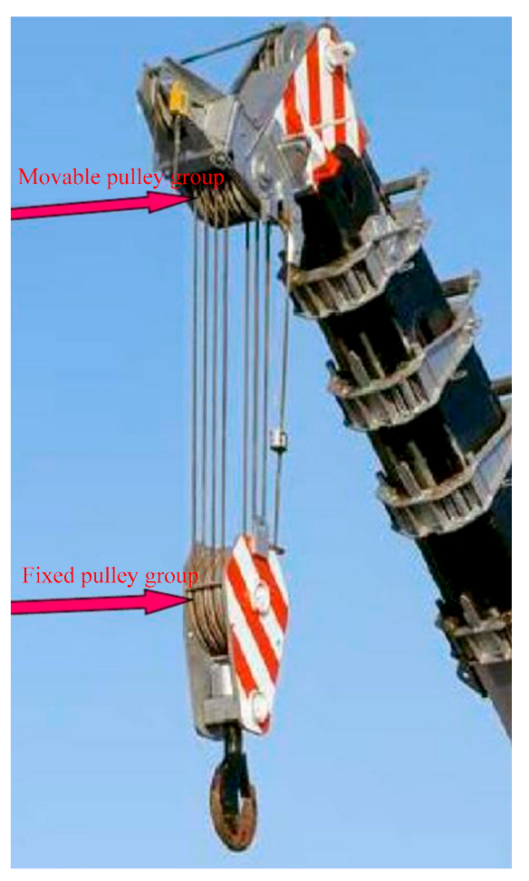
Optimal Placement of Sensors Based on Data Fusion for Condition Monitoring of Pulley Group under Speed Variation Condition

1
School of Mechanical Engineering, Anyang Institute of Technology, Anyang 455000, China
2
School of Mechanical Engineering, Xi’an Jiaotong University, Xi’an 710049, China
3
Mechanical and Electrical Engineering Department, Yuncheng University, Yuncheng 044000, China
*
Author to whom correspondence should be addressed.
Machines 2022, 10(2), 148; https://doi.org/10.3390/machines10020148
Submission received: 1 January 2022 / Revised: 14 February 2022 / Accepted: 15 February 2022 / Published: 17 February 2022
(This article belongs to the Special Issue Advances in Bearing Modeling, Fault Diagnosis, RUL Prediction)

Abstract

:
Pulley group plays an important role in the transmission of large mechanical equipment. To obtain informative data for condition monitoring, it is very important to optimize sensor placement on the pulley group. However, due to sharp speed fluctuation, heavy load and complex internal structure, sensor placement for acquiring optimal monitoring points is still a challenging task. Therefore, a novel sensor optimization method based on data fusion is proposed. In this method, the Kalman filter is firstly used to refine the collected signal for dealing with the variable noises. Subsequently, the variable periodicity strength of the signal is calculated to recognize the non-stationary characteristics of the measured signal. A data fusion technique based on maximum likelihood estimation (MLE) is then introduced to estimate sensitive components from the multi-source sensor signals for finding out optimal sensor placement points. The method is validated experimentally on a test rig of the pulley group with variable speed conditions. Analysis results show that the proposed method can recognize the optimal sensor placement points for the pulley group.

1. Introduction

The pulley group is the key structural component for transferring force and displacement in large mechanical equipment [1,2,3]. It can adjust the torque and motion with efficiency according to the specific need of users. In general, the pulley group works under heavy load and sharp speed fluctuation, which may lead to cause pulley failure and affect the safe operation of machinery. Therefore, it is very important to monitor the condition of the pulley group. Due to the long and complex vibration transmission path, selecting an appropriate data acquisition position plays a vital role in this process. Although sensor placement has long been investigated, those methods are rarely applicable to monitor pulley groups for the following reasons:
Firstly, it is always affected by environmental interference during the operation of machinery, and noise is a factor that should not be ignored [4]. Particularly, the pulley group usually suffers from strong variable load and sharp speed fluctuation in industrial applications. Thus, the noise interference experiences a sudden change in magnitude, and the corresponding power spectrum density (PSD) would not obey uniform distribution, as is assumed in the previous method [5,6]. It exhibits a strong non-Gaussian characteristic [7]. Therefore, a tool that can automatically track non-stationary changes and eliminate noise is needed here, since a conventional band-pass filter cannot eliminate noise interference from non-Gaussian characteristics [8].
Secondly, periodicity strength is a well adopted index for selecting the optimal measurement points. With this indicator, the optimal sensor location is determined by comparing the periodicity strengths of different measuring points [9,10,11]. However, this method is not suitable for sensor optimization under variable speed conditions, since the components of interest are smeared severely due to the frequency modulation effect in this condition.
Finally, the pulley group typically has several pullers on one axis, and it is also composed of movable and fixed forms together [12,13], as shown in Figure 1. Therefore, the measured signal is a mixture of vibrations from different sources. Since the traditional sensor optimal placement method is only applicable to single sources [14,15], they are no longer effective for the actuators with multi excitation sources, such as the pulley group. Moreover, the internal structure and transfer path of the pulley group are also very complex. This further hinders the optimal sensor placement for the pulley group [16,17].
Pulley groups usually work in harsh environments in industrial applications, and generally are fixed in a machine. Figure 2 shows the working conditions of pulley groups. To acquire the effective monitored data for the pulley group, sensor placement has the following requirements: (i) Health condition monitoring for the pulley group should be carried out by collecting the most comprehensive monitoring data with the least number of sensors, thus achieving the goal of adequate allocation for monitoring resources. (ii) The collecting health condition data should be reliable and effective so as to accurately grasp the running state of the pulley group, thereby providing a guarantee for the safe operation of machinery.
The above two targets put forward the requirement of economic practicability in industrial production for sensor optimal placement of the pulley group. Therefore, this paper takes into account the difficulties of a sensor configuration for the pulley group and proposes an optimal sensor placement technique based on data fusion. In this method, the Kalman filter is employed to deal with the non-stationary noise interference. Then, the variable periodicity strength of the denoised signal is processed by signal weighting to enhance the health condition characteristics of the monitored pulley group. Subsequently, the data fusion based on a maximum likelihood estimation (MLE) is introduced to produce the optimal sensitive signal of sensors. Finally, correlation analysis between the estimated sensitive signal and sensor collected signals is found to evaluate the optimal locations. In this way, the best sensor placements can be successfully identified for the health condition monitoring of the pulley group. Moreover, to verify the effectiveness of the achieved results, order spectrum analysis was performed in the proposed method.
The remaining of this paper is organized as follows. Theory background that forms the basis of the proposed sensor optimal placement technique is described in Section 2. The detail of the proposed method is provided in Section 3. The experiment results and statistic data analysis on a health condition monitoring of the pulley block under speed variation, are given in Section 4. The conclusion is drawn in Section 5.

2. Background of Theory

In this section, three theoretical aspects are introduced. They compose the basis of sensors’ optimal placement to the pulley group under speed variation conditions. The first approach is the Kalman filter, which can extract signals from non-stationary noise. Further, it is robust to the non-uniform distribution of PSD for non-stationary noise. The second method is the autocorrelation coefficient, which is capable of achieving the variable periodic strength for speed changing process. The last one is maximum likelihood estimation, which can estimate the sensitive signal in the condition of the existing multi-signal excitation source. The three techniques are detailed in the following, respectively.

2.1. Refining Signal by Kalman Filter

Under the variable conditions of speed and load, noise interference is changing with the signal. The corresponding PSD would not obey uniform distribution. Consequently, the conventional band-pass filter cannot handle noises in this condition for refining signal [18,19,20]. In view of this, the Kalman filter is employed to refine signals for dealing with noise interference due to its robust performance for the speed fluctuation and characteristic of excellent tracking signal [21,22,23].
For a discrete-time signal corrupted noise y ^ n , n = 1 , 2 , , N , the refined signal can be predicted as:
y n = F n y n 1 + B n u n
where y n 1 is the best refined signal in n − 1 th discrete point. y n is the coarse signal in nth discrete point according to y n 1 . F n is the signal transform matrix. B n is the control matrix. u n is the manipulated variable. Here, since the noise interference is a fluctuant condition, F n is a proportion matrix followed with speed variation.
Then, the signal transform equation can be calculated by:
P n = F n P n 1 F n T + Q
where P n 1 is the covariance of the predicted signal at the previous point. P n is the predicted covariance of the current discrete point based on P n 1 . Q denotes disturbance caused by the refinement model.
Therefore, the optimal refined signal can be denoted as:
y n = y n + K n z n H y n
where z n is the signals of current discrete point collected by sensors. H denotes the relationship between the current discrete point state and the signal acquired by the sensor. K n represents Kalman Gain and it can be calculated by:
K n = P n H T H P n H T + R 1
where R is the covariance of the collected signal by sensor.
To refine the next discrete point signal, the update equation is defined as:
P n + 1 = I K n + 1 H P n + 1
where I is the unit matrix.
Since the state of the sensor is fixed and the sampling interval is tiny in the process of data collection, the values of F n and H can be taken as 1, respectively. Meanwhile, there is no change of sensors during signal acquisition. Therefore, the values of B n and u n are set to 0, namely:
y n = F n y n 1
As a result, the refined non-stationary signal y n can be achieved according to the Kalman filter.

2.2. Variable Periodicity Strength Calculation

In the condition of speed variation, the signal exhibits a non-stationary characteristic, and its frequency spectrum appears as frequency modulation and spectral smearing [24,25]. Therefore, the periodicity of the signal is changing with speed variation. To deal with the variable condition, the rotor rotating a circle around the shaft is considered to be a complete period. Obviously, this is a period that varies with the speed of rotation. Moreover, the number of variable periods can be measured by an optical electronic transducer, which produces one pulse per revolution. In consequence, the variable periodicity strength of the signal can be calculated by the autocorrelation coefficient [9,26].
A refined signal with N discrete points can be defined as:
y n = y 0 , y 1 , y 2 , , y N 1 , n = 0 , 1 , 2 , , N 1
There are k pulses, and its variable periodicity strength can be calculated by:
C k = 1 N k σ x σ s n = 0 N k 1 y n μ x y n + k μ s
where μ x and μ s denote mean values of signal y n and y n + k , respectively. σ x and σ s are variances of signal y n and y n + k , respectively. Due to the non-stationary of signal, the trend of C k is towards to 1.

2.3. Maximum Likelihood Estimation

The pulley group usually contains some pulley components, thereby producing multiple signal excitation sources. In the test process, the collected signal measures information fused in all the excitation sources. It is a major difficulty to recognize sensitive signals containing health condition information from those signal sources comprised faults. Due to the feature of abnormal estimation [27], maximum likelihood estimation (MLE) is introduced to estimate the sensitive signal according to fused information [9,28]. For all the signals acquired from sensors, the ensemble of M discrete signals is given as follows:
Y n = y 1 n y 2 n y M n , n = 0 , 1 , 2 , , N 1
where y M n denotes signal collected by the Mth sensor. n is the discrete point of signal.
For the ith sensor, y i n is the output at discrete point n. Therefore, the collected signal y i n can be represented in the following form:
y i n = s n + w i n , i = 1 , 2 , , M
where s n is the signal, which is only contained condition information. w i n denotes the residual non-stationary noise interference after processing by the Kalman filter. Then, y i n is mapped into vector space:
y n = 1 s n + w n
where 1 R M is the unit matrix of transforming signal into vector. Here, w n = w 1 n w 2 n w M n is denoted as a noise vector of 1 × M.
Therefore, the sensitive signal of the sensor can be estimated by MLE:
s ¯ n = arg max s n p w n s n
where p w n s n is the likelihood function, which denotes the probability density function of non-stationary noise interference in the acquired signal by the sensor.
Rewriting Equation (11), the vector of noise interference can be obtained as follows:
w n = y n 1 s n
In consequence, the likelihood function can be given as [29]:
p w n s n = p w 1 n , w 2 n , w M n s n = p w 1 n s n × p w 2 n s n × × p w M n s n = i = 1 M 1 2 π σ i 2 exp 1 2 σ i 2 y i n s n 2
where σ i 2 denotes variance of the ith sensor collected signal.
Subsequently, taking logarithm to likelihood function can acquire the following equation:
log p w n s n = i = 1 M log 1 2 π σ i 2 y i n s n 2 2 σ i 2
To maximize the likelihood function of the signal, the first derivative of the logarithm is set to 0, namely:
s p w n s n = i = 1 M 1 σ i 2 y i n s n = 0
Finally, the sensitive signal of fusing all the sources can be given as follows:
s ¯ n = i = 1 M 1 σ i 2 1 i = 1 M 1 σ i 2 y i n , n = 1 , 2 , , N 1

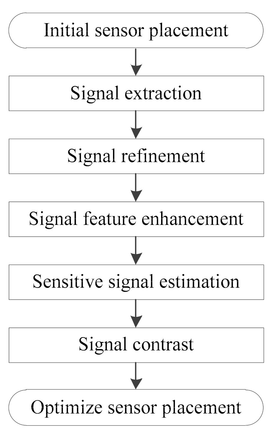
3. Procedure of the Proposed Optimal Sensor Placement Technique

To deal with the optimal placement of sensors for the pulley group under speed variation conditions, the proposed data fusion method is detailed in this section. The process is elaborated in Figure 3.

3.1. Initial Sensor Placement

The placement of initial measuring points is important in the optimal sensor placement. Based on different theories, it can be divided into two categories, sensor placement based on knowledge inference, and the analytical model [30,31]. According to the structure feature and non-stationary operating conditions of the real pulley group, there are the following factors: (1) The most vulnerable position where the pulley block is most likely to be damaged by force during operation are factors to be considered. (2) The nearest points in the parallel and orthogonal directions of the pulley shaft, i.e., the position and direction of the pulley block under the maximum rope force during operation are factors to be considered. Therefore, M sensors are arranged to the initial locations. In this process, sensors are arranged to build a wide and complete monitoring network, which lays the foundation for the subsequent optimal configuration of sensors.

3.2. Signal Extraction

Since all the sensors are on the same data acquisition card in the monitoring process for the pulley group, they are synchronized in terms of time instant. However, they are asynchronous on the phase due to the speed fluctuation. In this step, the ith sensor ( i 1 , M ) is assumed to have measured N points signal x i n ( n = 0 , 1 , , N 1 ) during the collection.
Since the collected signals are disturbed by the transmission path and noise, there are some differences in the process of oscillation and attenuation. Therefore, the collected signals are normalized before further processing.
As the median value is not affected by the attenuation process of amplitude, it is employed to represent the general level of data in this work. In addition, the signal peaks in x i n can be acquired by finding the rising edge or fail edge. Therefore, the median value of signal peaks is given as:
R i = m e d i a n p 1 , p 2 , , p j
Due to the effect of speed variation, the signal amplitude has experienced a process of up and coast down. As a result, to enhance the signal quality, the normalization factor of the ith sensor signal is determined as follows:
a i = max i = 1 , , M R i / R i
Therefore, the normalized signal for each sensor can be given as:
y ^ i n = a i x i n , n = 0 , 1 , , N 1

3.3. Signal Refinement

Though the amplitude of non-stationary noise interference has some reduction after signal normalization, the noise effect still cannot be ignored. Here, the Kalman filter with the time-varying feature detailed in Section 2.1 is used to process the normalized signal. In this way, the refined normalized signal y i n can be acquired.

3.4. Signal Feature Enhancement

Weighting can enhance the signal characteristics [32,33,34], therefore being performed to the variable periodicity strength elaborated in Section 2.2. After that, the proportion of single variable periodicity strength C i k in all the acquired signals can be shown as:
W i = C i i = 1 M C i
where M is the number of sensors, and i = 1 M W i = 1 .

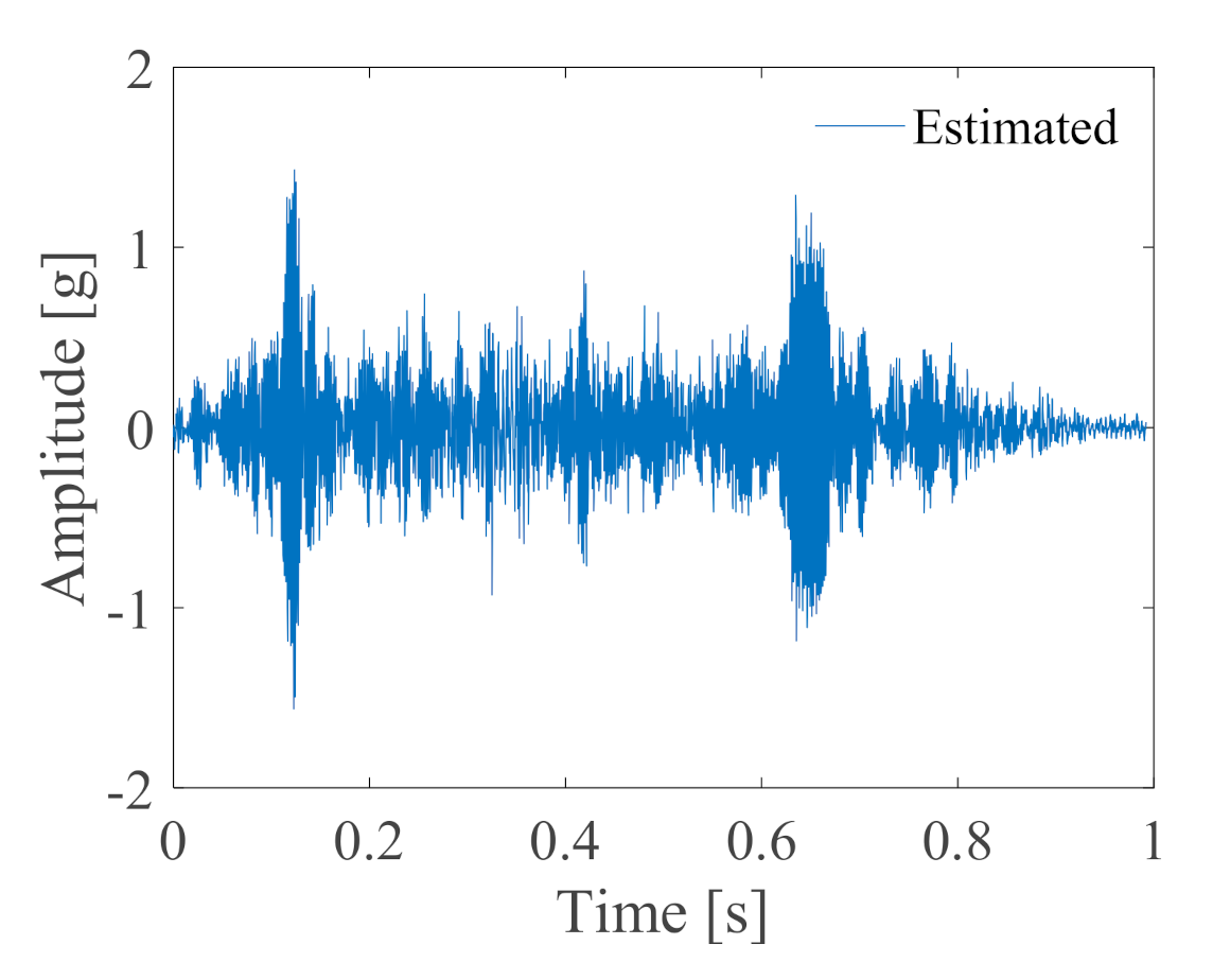
3.5. Sensitive Signal Estimation

After the aforementioned process, MLE is employed to the refined normalized signal y i n for estimating the sensitive signal. The detailed calculation is described in Section 2.3. To improve the estimated precision, the weighted factor W i achieved by the last steps are added into MLE. Therefore, the estimated sensitive signal is achieved by:
s ^ n = i = 1 M W i σ i 2 1 i = 1 M W i σ i 2 y i n , n = 1 , 2 , , N 1

3.6. Signal Contrast

In this step, correlation analysis based on parameter estimation [35,36] is performed between the estimated sensitive signal and the collected signals by sensors to evaluate the optimal loading position. In consequence, the contrast by a correlation coefficient of two signals is accomplished by the following equation:
r s ^ n , y i n = C o v s ^ n , y i n V a r s ^ n V a r y i n
where C o v s ^ n , y i n is the covariance between the estimated sensitive signal s ^ n and the collected signal y i n . V a r denotes variance.

3.7. Sensors Placement Evaluation

To find out effective sensor loading locations, signal contrast results about value r s ^ n , y i n are checked. As a result, the greater the value r s ^ n , y i n , the greater the correlation between the estimated sensitive signal and ith collected sensor signal. Namely, the position of the ith sensor is closer to the key monitoring point.
Through many tests, the correlation coefficient between the estimated sensitive signal and each collected sensor signal is obtained. Then, the optimal sensor location can be obtained by statistical analysis.

4. Experimental Validations on Transient Conditions

4.1. Experiment Setup

In view of the difficulty in monitoring the pulley group of large mechanical equipment, in this step, a test rig simulating the pulley block in the crane was employed to verify the proposed method. The test rig system is shown in Figure 4. It contains four parts: the servo motor with 1.5 KW, the servo drive system, the pulley group system, and the load system. Moreover, a coco-80 dynamic signal acquisition instrument is used to collect signals. KISTLER acceleration transducers and a tachometer transducer are mounted on the test rig for measurement. In the pulley group, the angular contact ball bearings are connected to the inner ring of the pulley through an interference fit. The geometric parameters of bearing are listed in Table 1. The normalized bearing characteristic frequency (NBCFs), in order, contained ball pass frequency of outer race (BPFO), ball pass frequency of inner race (BPFI) and ball spin frequency (BSF), are given in Table 2.
In this process, bearings with outer and inner damages are used to simulate the monitored faults. Figure 5 shows the corresponding fault bearings. The fault degrees are the depth of bearing damage, which is 0.15 mm and 0.05 mm, respectively. The faulty bearing is assembled in the first pulley shown in Figure 4. The speed variation conditions are conducted by six types, and the maximum rotation speed of the pulley is ranging from 1200 to 2500 (rpm). The sampling frequency is set to 25.6 kHz during the test. Sensors are initially arranged in the positions shown in Figure 4. A tachometer provided pulse signals to measure the variable period.

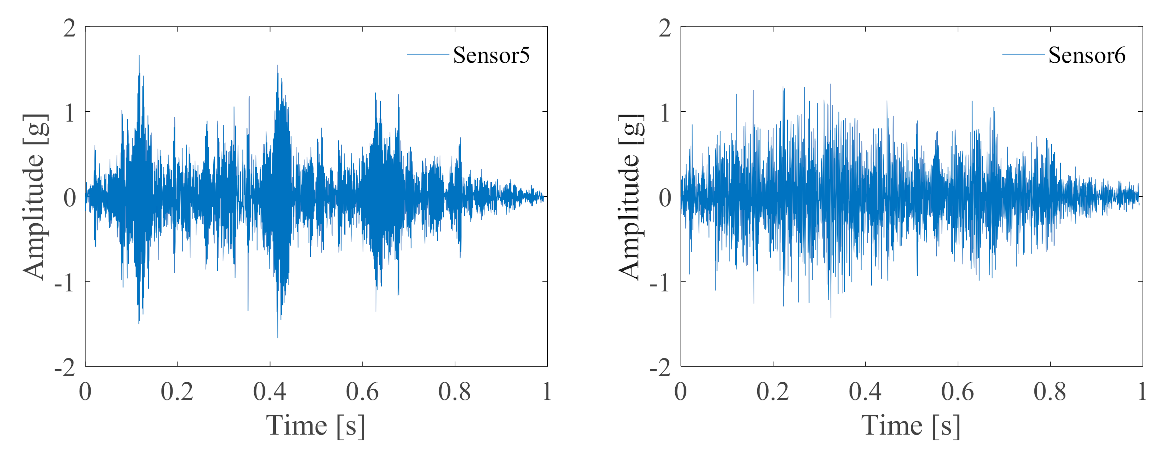
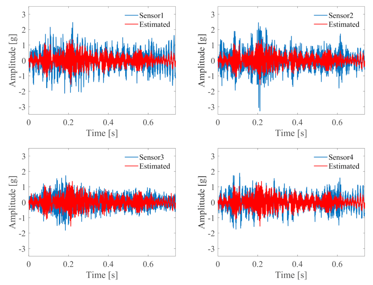
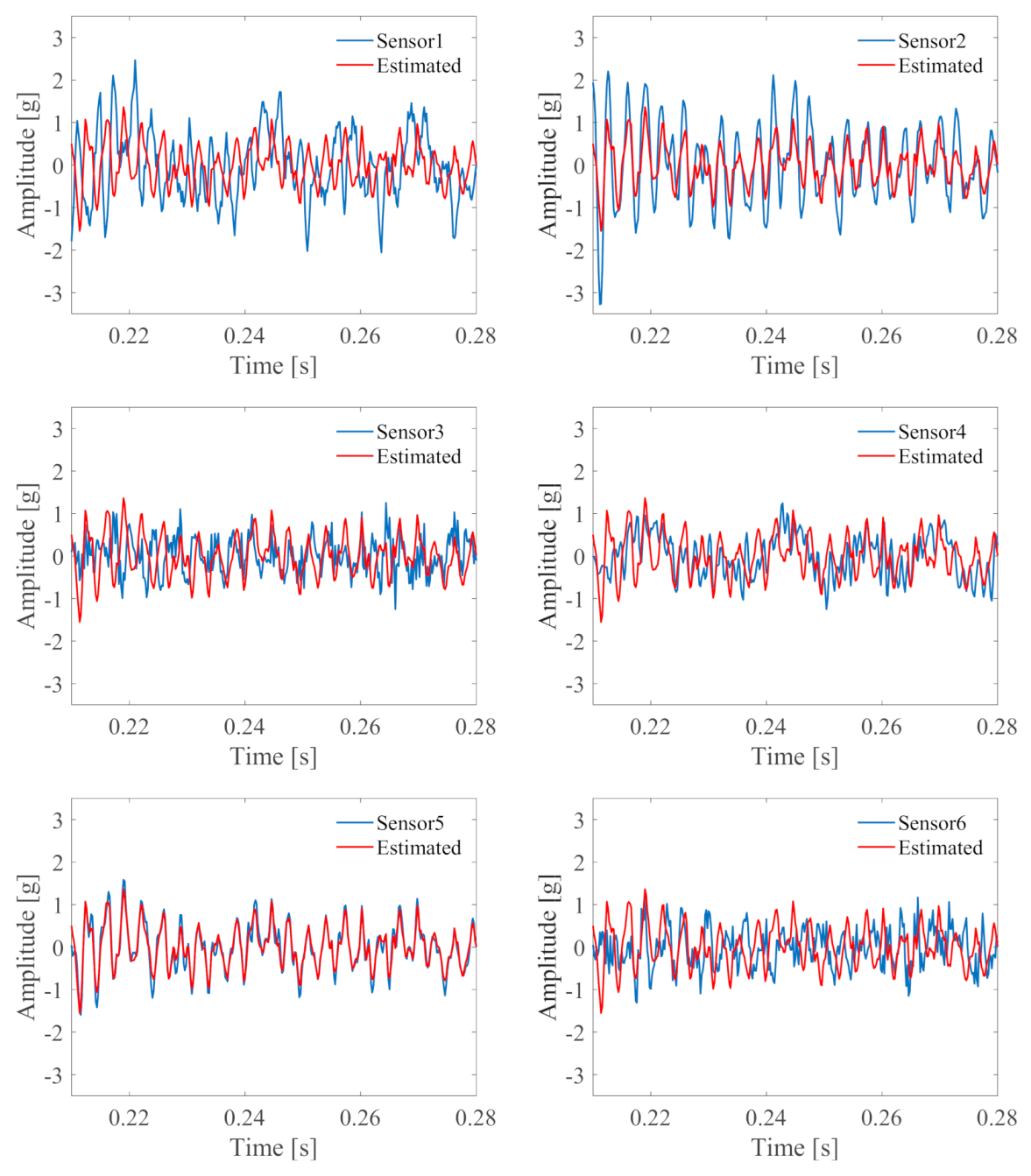
4.2. Data Processing and Verification

In this experiment, an outer fault with a depth of 0.15 mm is analyzed under the maximum rotation speed of 2000 (rpm). Figure 6 gives the corresponding pulse signal, which denotes that this bearing signal has 23 variable periods. The pulley group experiences a fast speed-up and coast-down process. Signals are collected by sensors as described above. Through extraction and refinement, the processed signals are given in Figure 7. Then, the sensitive signal is estimated by MLE, and it is illustrated in Figure 8.
Subsequently, the estimated sensitive signal is performed correlation analysis with the collected signals for contrasting. The correlation coefficients are obtained by r 1 = 0.5829 , r 2 = 0.02877 , r 3 = 0.14892 , r 4 = 0.92297 , r 5 = 0.16231 and r 6 = 0.034755 . From those values, the maximum correlation is the fourth sensor. The contrasting results are shown in Figure 9, respectively. To present clearly, the zoomed signals in 0.62–0.67 s are extracted to display in Figure 10. From this figure, the signal of the fourth sensor well agrees with the estimated one. Therefore, it can be concluded that the collected fourth signal is the best one in this test process.
To further validate the effectiveness, order spectrum analysis [37,38] is employed for the collected signals. Figure 11 shows the corresponding envelope order spectrums of those bearing signals. From this figure, BPFO can be clearly identified. In particular, the amplitude of the order spectrum acquired from the fourth signal is higher than the others. It just proves the conjecture that the fourth sensor placement point is the optimal location for this test experiment. Therefore, the conjecture for the optimal sensor in this test process is right. Finally, many independent tests are performed to analyze the correlation between the estimated signal and sensors’ collected signals under different maximum rotation speeds. The data statistics of correlation are given in Table 3. From the statistical results, it can reveal that the effective sensor placements are located in the first, second, fourth, and fifth sensors. Hence, the four sensor placement points might be ideal for this bearing health condition monitoring.
The above tests are only outer race fault monitoring of bearing in the pulley group. Next, the inner race fault tests are used to verify the proposed method. A defective bearing with a depth of 0.05 mm in the inner race is installed on the first pulley. Sensor placement is still adopted in the above initial scheme. Figure 12 shows the collected pulse signal, thereby obtaining the number of variable periods. The signals acquired by sensors are performed refinement operation according to the Kalman filter. The results are given in Figure 13. Via the MLE algorithm, the sensitive signal is estimated and illustrated in Figure 14.
Then, signal contrast is implemented between the estimated sensitive signal and the collected signals. The compared results are given in Figure 15. The corresponding correlation coefficients of contrasted signals are r 1 = 0.030564 , r 2 = 0.57096 , r 3 = 0.023839 , r 4 = 0.36198 , r 5 = 0.92309 and r 6 = 0.036917 , respectively. The maximum correlation is the fifth sensor. Moreover, Figure 16 shows the zoomed signals in 0.21–0.28 s. It is clear that the estimated sensitive signal is heavily agreeing with the collected signal of sensor 5. Therefore, it is reasonable to conclude that the best placement is the location of sensor 5 in this test experiment.
Subsequently, order spectrum analysis is further used to verify the correctness of the conjectural optimal sensor placement point, and the envelope order spectrums that come from the collected bearing signals are shown in Figure 17. From this figure, the maximum amplitude of the order spectrum is the fifth collected signal, while the others do not even show any NBCFs. This is exactly the same as the previous reasoning about optimal sensor placement. To effectively check out all the sensor sensitive location points, a great deal of test experiments have been carried out. The data statistical results of correlation analysis between the estimated sensitive signal and the collected signals are given in Table 4. It is clearly shown the maximum correlation coefficients are concentrated in the first, second, fourth, and fifth sensors. Therefore, it can be concluded that these acquired optimal sensor placement points might be considered in the test process.
Based on the data statistical results of the aforementioned correlation coefficients, the optimal sensor placement for the health condition monitoring of the pulley group can be concluded as the first, second, fourth, and fifth sensors. Therefore, the proposed optimal sensor placement technique can help to check out the optimal health condition monitoring points for the pulley group under speed variation.

5. Conclusions

This paper proposed a sensor optimization method for pulley group condition monitoring under speed variations. After the refinement based on the Kalman filter, the non-stationary noise interference is reduced. Then, variable periodicity strength calculated by autocorrelation analysis of the collected signal is performed to recognize the signal characteristic. Subsequently, the sensitive signal with maximum fault features is estimated by MLE. Finally, correlation analysis is implemented between the estimated sensitive signal and the collected signals to find out the optimal sensor placements. To verify the obtained results, order spectrum analysis is performed on the collected signals. Through the data statistics of many experiments, all the sensitive sensor layout points are identified. In the experiment, the proposed sensor optimal placement algorithm is applied to the bearing condition monitoring of the pulley group under speed fluctuation. It is found that the effective placements of sensors can be more accurately identified by this method.

6. Discussions

In this paper, a method of optimal selection of sensor measuring points for monitoring actual pulley blocks is proposed. Through this work, we can provide a method to select the best measuring point for monitoring the pulley block with a similar shape in the actual project. Meanwhile, a technical solution for the optimal placement of sensors under the same working condition based on this technology can be provided. However, since this method is designed to solve practical engineering problems, it is difficult to construct a theoretical model of monitoring objects, which makes it impossible to compare and verify the methods. At the same time, due to the need for practical engineering, there is still a lack of further research on the innovation of methods. Therefore, in future research, we should deepen the construction of practical engineering and theoretical models, draw lessons from existing methods and technologies, focus on problems, and make more in-depth theoretical innovations.

Author Contributions

Conceptualization, J.W. and Y.Z.; methodology, J.W. and Y.Z.; software, J.W. and H.M.; validation, J.W., Y.W. and X.X.; formal analysis, J.W.; investigation, J.W. and Y.Z.; resources, J.W. and Y.Z.; data curation, J.W. and Y.Z.; writing—original draft preparation, J.W. and Y.Z.; writing—review and editing, J.W. and Y.Z.; visualization, J.W. and X.X; supervision, J.W. and Y.Z.; project administration, J.W. and H.M.; funding acquisition, J.W. and Y.Z. All authors have read and agreed to the published version of the manuscript.

Funding

This work is supported financially by the National Natural Science Foundation of China (Grant No. 51775411) and the Key Scientific and Technological Project of Henan Province (Grant No. 202102210264).

Data Availability Statement

Not applicable.

Acknowledgments

Comments and suggestions from the editor and reviewers are very much appreciated.

Conflicts of Interest

The authors declare no conflict of interest.

References

  1. Jiang, K.; Zhou, Y.; Han, L.; Li, L.; Liu, Y.; Hu, S. Design of a high-resolution instantaneous torque sensor based on the double-eccentric modulation principle. IEEE Sens. J. 2019, 19, 6595–6601. [Google Scholar] [CrossRef]
  2. Urda, P.; Aceituno, J.F.; Muñoz, S.; Escalona, J.L. Artificial neural networks applied to the measurement of lateral wheel-rail contact force: A comparison with a harmonic cancellation method. Mech. Mach. Theory 2020, 153, 103968. [Google Scholar] [CrossRef]
  3. Li, C.; Liu, X.; Tang, Q.; Chen, Z. Modeling and nonlinear dynamics analysis of a rotating beam with dry friction support boundary conditions. J. Sound Vib. 2021, 498, 115978. [Google Scholar] [CrossRef]
  4. Ghayem, F.; Rivet, B.; Farias, R.C.; Jutten, C. Robust Sensor Placement for Signal Extraction. IEEE Trans. Signal Process. 2021, 69, 4513–4528. [Google Scholar] [CrossRef]
  5. Martin, R. Noise power spectral density estimation based on optimal smoothing and minimum statistics. IEEE Trans. Speech Audio. Process. 2001, 9, 504–512. [Google Scholar] [CrossRef] [Green Version]
  6. Tan, Y.; Guo, L.; Gao, H.; Zhang, L. Deep Coupled Joint Distribution Adaptation Network: A Method for Intelligent Fault Diagnosis Between Artificial and Real Damages. IEEE Trans. Instrum. Meas. 2020, 70, 1–12. [Google Scholar] [CrossRef]
  7. Krause, A.; Singh, A.; Guestrin, C. Near-optimal sensor placements in Gaussian processes: Theory, efficient algorithms and empirical studies. J. Mach. Learn. Res. 2008, 9, 235–248. [Google Scholar]
  8. Zhang, H.; Ayoub, R.; Sundaram, S. Sensor selection for Kalman filtering of linear dynamical systems: Complexity, limitations and greedy algorithms. Automatica 2017, 78, 202–210. [Google Scholar] [CrossRef]
  9. Duro, J.A.; Padget, J.A.; Bowen, C.R.; Kim, H.A.; Nassehi, A. Multi-sensor data fusion framework for CNC machining monitoring. Mech. Syst. Signal Processing 2016, 66, 505–520. [Google Scholar] [CrossRef] [Green Version]
  10. Fortino, G.; Galzarano, S.; Gravina, R.; Li, W. A framework for collaborative computing and multi-sensor data fusion in body sensor networks. Inf. Fusion 2015, 22, 50–70. [Google Scholar] [CrossRef]
  11. Downey, A.; Hu, C.; Laflamme, S. Optimal sensor placement within a hybrid dense sensor network using an adaptive genetic algorithm with learning gene pool. Struct. Heal. Monit. 2018, 17, 450–460. [Google Scholar] [CrossRef] [Green Version]
  12. Bayat, A.; Shaaban, H.; Giakas, G.; Lees, V.C. The pulley system of the thumb: Anatomic and biomechanical study. J. Hand Surg. 2002, 27, 628–635. [Google Scholar] [CrossRef]
  13. Liu, X.; El Naggar, M.H.; Wang, K.; Wu, J. Three-dimensional axisymmetric analysis of pile vertical vibration. J. Sound Vib. 2021, 494, 115881. [Google Scholar] [CrossRef]
  14. Isaacs, J.T.; Klein, D.J.; Hespanha, J.P. Optimal sensor placement for time difference of arrival localization. In Proceedings of the Proceedings of the 48h IEEE Conference on Decision and Control (CDC) Held Jointly with 2009 28th Chinese Control Conference, Shanghai, China, 15–18 December 2019; pp. 7878–7884. [Google Scholar]
  15. Liu, C.Q.; Ding, Y.; Chen, Y. Optimal coordinate sensor placements for estimating mean and variance components of variation sources. IIE Trans. 2005, 37, 877–889. [Google Scholar] [CrossRef]
  16. Yi, T.-H.; Li, H.-N.; Gu, M. A new method for optimal selection of sensor location on a high-rise building using simplified finite element model. Struct. Eng. Mech. 2011, 37, 671–684. [Google Scholar] [CrossRef]
  17. Argyris, C.; Papadimitriou, C.; Panetsos, P. Bayesian Optimal Sensor Placement for Modal Identification of Civil Infrastructures. J. Smart Cities 2017, 2, 69–86. [Google Scholar] [CrossRef]
  18. Zhao, M.; Lin, J.; Wang, X.; Lei, Y.; Cao, J. A tacho-less order tracking technique for large speed variations. Mech. Syst. Signal Process. 2013, 40, 76–90. [Google Scholar] [CrossRef]
  19. Jiang, K.; Zhou, Y.; Chen, Q.; Han, L. In Processing Fault Detection of Machinery Based on Instantaneous Phase Signal. IEEE Access 2019, 7, 123535–123543. [Google Scholar] [CrossRef]
  20. Guo, L.; Lei, Y.; Li, N.; Yan, T.; Li, N. Machinery health indicator construction based on convolutional neural networks considering trend burr. Neurocomputing 2018, 292, 142–150. [Google Scholar] [CrossRef]
  21. Piat, E.; Abadie, J.; Oster, S. Nanoforce estimation based on Kalman filtering and applied to a force sensor using diamagnetic levitation. Sensors Actuators A Phys. 2012, 179, 223–236. [Google Scholar] [CrossRef] [Green Version]
  22. Wu, J.; Wang, Z.; Zhang, L. Unbiased-estimation-based and computation-efficient adaptive MPC for four-wheel-independently-actuated electric vehicles. Mech. Mach. Theory 2020, 154, 104100. [Google Scholar] [CrossRef]
  23. Ricciardi, T.R.; Wolf, W.R.; Moffitt, N.J.; Kreitzman, J.R.; Bent, P. Numerical noise prediction and source identification of a realistic landing gear. J. Sound Vib. 2021, 496, 115933. [Google Scholar] [CrossRef]
  24. Wu, J.; Zi, Y.; Chen, J.; Zhou, Z. A modified tacho-less order tracking method for the surveillance and diagnosis of machine under sharp speed variation. Mech. Mach. Theory 2018, 128, 508–527. [Google Scholar] [CrossRef]
  25. Schmidt, S.; Heyns, P.; De Villiers, J. A tacholess order tracking methodology based on a probabilistic approach to incorporate angular acceleration information into the maxima tracking process. Mech. Syst. Signal Process. 2018, 100, 630–646. [Google Scholar] [CrossRef] [Green Version]
  26. Jing, L.; Zhao, M.; Li, P.; Xu, X. A convolutional neural network based feature learning and fault diagnosis method for the condition monitoring of gearbox. Measurement 2017, 111, 1–10. [Google Scholar] [CrossRef]
  27. Myung, I.J. Tutorial on maximum likelihood estimation. J. Math. Psychol. 2003, 47, 90–100. [Google Scholar] [CrossRef]
  28. Fisher, M.R.A. On the mathematical foundations of theoretical statistics. Phil. Trans. R. Soc. Lond. A 1922, 222, 309–368. [Google Scholar]
  29. Pan, J.-X.; Fang, K.-T. Maximum Likelihood Estimation, Growth Curve Models and Statistical Diagnostics; Springer: Berlin/Heidelberg, Germany, 2002; pp. 77–158. [Google Scholar]
  30. Ghayem, F.; Rivet, B.; Jutten, C.; Farias, R.C. Gradient-based algorithm with spatial regularization for optimal sensor placement. In Proceeding of the ICASSP 2020–2020 IEEE International Conference on Acoustics, Speech and Signal Processing (ICASSP), Barcelona, Spain, 4–8 May 2020; pp. 5655–5659. [Google Scholar]
  31. Lee, K.; Byun, N.; Shin, D.H. A Damage Localization Approach for Rahmen Bridge Based on Convolutional Neural Network. KSCE J. Civ. Eng. 2019, 24, 1–9. [Google Scholar] [CrossRef]
  32. Zeng, Q.; Vasudevan, V.; Ramanathan, C.; Jia, P. Non-Local Mean Filtering for Electrophysiological Signals. U.S. Patent No. 9,974,458, 22 May 2018. [Google Scholar]
  33. Dietrich, P.F.; Davi, G.S.; Friday, R.J. Location of Wireless Nodes Using Signal Strength Weighting Metric. U.S. Patent No. 7,116,988, 3 October 2006. [Google Scholar]
  34. Mabkhot, M.M.; Darmoul, S.; Al-Samhan, A.M.; Badwelan, A. A Multi-Criteria Decision Framework Considering Different Levels of Decision-Maker Involvement to Reconfigure Manufacturing Systems. Machines 2020, 8, 8. [Google Scholar] [CrossRef] [Green Version]
  35. Cohen, P.; West, S.G.; Aiken, L.S. Applied Multiple Regression/Correlation Analysis for the Behavioral Sciences; Psychology Press: New York, NY, USA, 2014. [Google Scholar]
  36. Mukaka, M.M. Statistics corner: A guide to appropriate use of correlation coefficient in medical research. Malawi. Med. J. 2012, 24, 69–71. [Google Scholar] [PubMed]
  37. Zhao, M.; Lin, J.; Xu, X.; Lei, Y. Tacholess Envelope Order Analysis and Its Application to Fault Detection of Rolling Element Bearings with Varying Speeds. Sensors 2013, 13, 10856–10875. [Google Scholar] [CrossRef]
  38. Jiang, K.; Han, L.; Zhou, Y. Quantitative evaluation of the impurity content of grease for low-speed heavy-duty bearing using an acoustic emission technique. Meas. Control 2019, 52, 1159–1166. [Google Scholar] [CrossRef] [Green Version]
Figure 1. Pulley group without shell.
Machines 10 00148 g001
Figure 2. Working conditions of pulley groups.
Machines 10 00148 g002
Figure 3. Flow chart of the data fusion method.
Machines 10 00148 g003
Figure 4. The test rig system of the Pulley group.
Machines 10 00148 g004
Figure 5. Fault bearings used in the experiment.
Machines 10 00148 g005
Figure 6. Pulse signal collected in outer race fault experiment.
Machines 10 00148 g006
Figure 7. Processed signals in outer race fault experiment.
Machines 10 00148 g007aMachines 10 00148 g007b
Figure 8. Estimated sensitive signal in outer race fault experiment.
Machines 10 00148 g008
Figure 9. Contrasted results between estimated and collected signals in outer race fault experiment.
Machines 10 00148 g009
Figure 10. Contrasted results zoomed in 0.62–0.67 s in outer race fault experiment.
Machines 10 00148 g010
Figure 11. Envelope order spectrums of the collected signals in outer race fault experiment.
Machines 10 00148 g011
Figure 12. Pulse signal in inner race fault experiment.
Machines 10 00148 g012
Figure 13. Processed signals in inner race fault experiment.
Machines 10 00148 g013
Figure 14. Estimated sensitive signal in inner race fault experiment.
Machines 10 00148 g014
Figure 15. Contrasted results between estimated and real signals in inner race fault experiment.
Machines 10 00148 g015aMachines 10 00148 g015b
Figure 16. Contrasted results zoomed in 0.21–0.28 s in inner race fault experiment.
Machines 10 00148 g016
Figure 17. Envelope order spectrums of the collected signals in inner race fault experiment.
Machines 10 00148 g017
Table 1. Parameters of angular contact ball bearing in the test.
Roller Diameter (mm)Pitch Diameter (mm)Contact Angle (Degree)Number of Rollers
625158
Table 2. NBCFs of the angular contact ball bearing.
ItemsNBCFs in Order
BPFO3.0727
BPFI4.9272
BSF1.9714
Table 3. Data managements about correlation coefficients for signal contrast (Outer race fault).
Sensor
123456
Fault deep 0.15 mm
Rotation speed: 1200 rpm
10.83780.651180.118720.794890.43821−0.092311
2−0.043148−0.218160.0836490.687460.26696−0.064068
30.811710.633770.117130.757720.39468−0.0821
40.881340.773050.102730.864650.65758−0.065752
Rotation speed: 1500 rpm
1−0.133190.184590.2272−0.141220.809720.17178
20.384690.86491−0.14787−0.0213570.0147710.24464
3−0.0042855−0.197810.25310.89836−0.21098−0.1662
4−0.11907−0.217350.273940.146330.837210.049634
Rotation speed: 1800 rpm
10.0147260.54459−0.171950.0762770.773620.33751
20.353030.44771−0.0963970.292010.824860.25566
30.198180.48196−0.214510.13790.80960.33548
4−0.120760.66541−0.23356−0.160560.600310.45627
Rotation speed: 2000 rpm
10.0520650.7064−0.048851−0.495950.576920.28651
2−0.5829−0.028770.148920.92297−0.162310.034755
30.486120.364570.0505860.532980.852740.15909
40.263480.53061−0.260520.284570.806960.30294
Rotation speed: 2200 rpm
10.332390.141540.065250.547390.85870.19482
20.702720.592150.144370.53196−0.22917−0.14489
30.339190.27357−0.036020.473370.94450.12273
40.4670.247030.0369920.644290.84770.16971
Rotation speed: 2500 rpm
10.853010.668820.176580.821620.28622−0.18471
20.850880.696990.18640.830020.44305−0.14017
30.83170.62770.0873780.772670.11598−0.10468
40.48575−0.0358840.213630.784740.226050.065409
Fault deep 0.05 mm
Rotation speed: 1200 rpm
1−0.56671−0.19487−0.024053−0.0545720.621780.38272
2−0.36415−0.27012−0.00837730.364070.664050.34641
30.7520.633080.0651640.45277−0.052138−0.23672
40.82170.654580.0319420.723590.28336−0.13674
Rotation speed: 1500 rpm
1−0.152530.331230.255960.267640.83146−0.020051
2−0.179530.168430.201280.627370.667170.07225
30.0843640.0460280.218140.76107−0.163350.10599
4−0.172270.445140.170060.740560.167860.0033331
Rotation speed: 1800 rpm
10.934670.43286−0.0413340.778310.24774−0.10228
20.897960.61790.0112830.840890.64185−0.054629
30.924330.68623−0.0477050.902950.55805−0.097335
40.902960.654490.0738670.860050.60988−0.076486
Rotation speed: 2000 rpm
10.907580.642510.000886410.857780.65353−0.12146
20.684430.632610.151010.33907−0.29137−0.16928
30.856860.63724−0.0104710.707410.3065−0.090043
4−0.523380.0420150.124850.92774−0.0816680.036343
Rotation speed: 2200 rpm
10.866250.682430.0617610.763090.28737−0.11667
20.866540.64276−0.102360.791730.1828−0.067055
30.839130.720180.0509050.728790.40057−0.086646
4−0.275760.316140.157220.808760.259020.027931
Rotation speed: 2500 rpm
10.911120.701280.00108630.886140.47057−0.11252
20.92646−0.0897780.078002−0.36902−0.0444640.036145
30.925460.61891−0.0568250.850570.39395−0.017999
40.899490.67274−0.0313940.851010.32548−0.026165
Table 4. Data management of correlation coefficients for signal contrast (Outer race fault).
Sensor
123456
Fault deep 0.15 mm
Rotation speed: 1200 rpm
10.852220.808940.146560.83170.7761−0.12351
20.6350.759660.0217780.15385−0.23207−0.15742
30.849310.809690.0976730.832210.7561−0.094068
40.579790.807720.393490.248280.30959−0.32808
Rotation speed: 1500 rpm
1−0.0898830.750020.0902070.52179−0.028005−0.012712
2−0.0471190.879010.10420.452170.20205−0.084225
30.54340.89041−0.00134360.328290.209080.00045367
40.611240.8546−0.108850.39090.10330.031138
Rotation speed: 1800 rpm
10.72290.76080.0127590.562290.40134−0.040798
20.699860.80329−0.0737160.447890.22955−0.056911
3−0.0730060.89297−0.081045−0.044191−0.216830.27441
40.626770.808440.0383520.26570.31363−0.059033
Rotation speed: 2000 rpm
10.280860.78433−0.0655030.568020.443630.13578
2−0.38273−0.0311480.063020.566220.279280.33542
3−0.148530.37444−0.0334630.652760.435240.28784
40.777260.79265−0.0107740.653490.36161−0.06578
Rotation speed: 2200 rpm
10.16433−0.409930.212640.505070.16620.23851
20.732820.794970.0287730.556050.25377−0.043044
30.65540.803580.0763630.393020.22082−0.098408
4−0.33601−0.23633−0.0731960.473260.53840.3367
Rotation speed: 2500 rpm
10.821710.791820.0259220.765550.4813−0.03199
20.789610.775210.0278780.714270.40341−0.066361
30.490030.149030.282020.544630.539120.19294
40.455720.154630.272970.515570.530710.22422
Fault deep 0.05 mm
Rotation speed: 1200 rpm
10.472240.396880.0031098−0.365720.70526−0.10261
20.731950.397990.056075−0.192510.33247−0.11556
30.850110.7358−0.240760.881440.855580.017053
40.649490.22980.11320.736720.49208−0.14148
Rotation speed: 1500 rpm
1−0.2455−0.132810.0649960.88644−0.0117250.079
2−0.242290.0817540.0457350.889460.0414050.12309
3−0.30565−0.0295880.0318720.88732−0.020270.14228
4−0.29568−0.148330.0226110.91927−0.1140.12348
Rotation speed: 1800 rpm
1−518560.128510.0316890.800880.236750.14782
2−0.544230.0350930.0122660.715990.225330.15864
30.7953−0.0519340.00107350.439610.261380.21675
40.74131−0.120230.0301040.67233−0.0859430.15108
Rotation speed: 2000 rpm
1−0.413930.43174−0.0812230.162170.728190.2286
2−0.465230.292170.151860.80546−0.020250.2303
30.688070.0052640.0331710.429760.293250.29485
4−0.67026−0.106620.0605860.77671−0.112050.21197
Rotation speed: 2200 rpm
1−0.49894−0.018890.0262080.91044−0.0654450.11508
20.594370.651670.0287770.469760.70036−0.13214
3−0.516330.031794−0.0010650.92324−0.120450.14602
4−0.459870.38318−0.157350.180960.783550.21148
Rotation speed: 2500 rpm
10.835510.628070.151120.600590.42709−0.1545
20.0305640.570960.0238390.361980.923090.036917
30.662330.62634−0.0476390.603110.7225−0.07839
4−0.159390.23821−0.14850.283160.910780.22182
Publisher’s Note: MDPI stays neutral with regard to jurisdictional claims in published maps and institutional affiliations.

