Article

A Novel Learning Based Non-Lambertian Photometric Stereo Method for Pixel-Level Normal Reconstruction of Polished Surfaces

1
State Key Laboratory of Fluid Power and Mechatronic Systems, School of Mechanical Engineering, Zhejiang University, Hangzhou 310027, China
2
Key Laboratory of Advanced Manufacturing Technology of Zhejiang Province, School of Mechanical Engineering, Zhejiang University, Hangzhou 310027, China
*
Author to whom correspondence should be addressed.
Machines 2022, 10(2), 120; https://doi.org/10.3390/machines10020120
Submission received: 9 January 2022 / Revised: 31 January 2022 / Accepted: 2 February 2022 / Published: 8 February 2022
(This article belongs to the Special Issue Precision Measurement and Machines)

Abstract

:
High-quality reconstruction of polished surfaces is a promising yet challenging task in the industrial field. Due to its extreme reflective properties, state-of-the-art methods have not achieved a satisfying trade-off between retaining texture and removing the effects of specular outliers. In this paper, we propose a learning based pixel-level photometric stereo method to estimate the surface normal. A feature fusion convolutional neural network is used to extract the features from the normal map solved by the least square method and from the original images respectively, and combine them to regress the normal map. The proposed network outperforms the state-of-the-art methods on the DiLiGenT benchmark dataset. Meanwhile, we use the polished rail welding surface to verify the generalization of our method. To fit the complex geometry of the rails, we design a flexible photometric stereo information collection hardware with multi-angle lights and multi-view cameras, which can collect the light and shade information of the rail surface for photometric stereo. The experimental results indicate that the proposed method is able to reconstruct the normal of the polished surface at the pixel level with abundant texture information.

1. Introduction

Surface quality inspection of products is an essential part of industrial manufacturing [1]. In recent years, 2D and 3D machine vision have become the mainstream methods to obtain the surface information of objects, enabling automatic surface defect detection and size measurement of industrial products [2,3,4,5]. However, obtaining information of surface with specular reflection is still a challenging task, especially in the industrial field [6]. Because the reflected light from the specular reflection area is more significant than the corresponding threshold of the camera sensors, the specular reflection area in the image obtained by the traditional 2D vision is overly highlighted and barely contains any useful information. In contrast, 3D vision can obtain the depth of the object surface and reflect the surface characteristics more comprehensively and concisely, thus becoming the commonly used method to replace 2D vision in the industrial field [7]. The mainstream 3D vision in the industrial field includes binocular stereo vision, structured light, time-of-flight (TOF), and so forth, which have been applied to 3D-dimension measurement and surface defect detection [8,9]. However, these methods are costly and can hardly deal with small surface defects.
In recent years, photometric stereo has become a very promising technology in 3D vision due to various outstanding advantages [10], among which three deserve our attention. The first is pixel-level resolution. Photometric stereo can reconstruct the normal of each pixel with rich texture information. The second is that it can handle specular reflections. Photometric stereo is a technology based on the reflection of the object surface. The normal of the specular reflection area can be regarded as the bisector of the viewing and light directions. Furthermore, the use of multiple images to reconstruct the normal map can greatly reduce the adverse effects of the highlighted area. The third is low cost. In terms of hardware, photometric stereo only requires one camera and multiple LED lights. Therefore, a large amount of research on photometric stereo has been carried out, and preliminary applications have been obtained in many fields, such as the detection of defects on the surface of strip steel [11].
The main problem that limits the development and application of photometric stereo is the estimation of non-Lambertian surface normals. The classic photometric stereo technology was developed based on the Lambertian reflectance model [12], but a pure Lambertian surface rarely exists in reality. As a result, numerous research papers have extended photometric stereo to non-Lamberttian fields. Non-Lambertian photometric stereo methods can be roughly divided into four categories. The first category is based on the method of removing outliers. The earliest non-Lambertian photometric stereo method believes that specular reflection rarely exists in photometric stereo, which is an abnormal value. Methods such as rank minimization [13], RANSAC [14], taking median values [15], expectation maximization [16], and sparse Bayesian regression [17] have been proposed to eliminate outliers in observations and estimate relatively accurate normal maps. However, such a method is only suitable for the case in which a small number of non-Lambertian regions exist. For materials with a large amount of specular reflection such as metal surfaces, these methods are no longer applicable. The second category is based on sophisticated reflectance models. These methods accurately estimate the surface normal by establishing the reflection model of the object surface, including many classic analysis models, such as the Blinn–Phong model [18], the Torrance–Sparrow model [19], the Ward model [20], the Cook–Torrance model [21] and so on. Some methods based on improved BRDF have been proposed, such as bivariate BRDF representations [22,23] and symmetry-based approach [24], which are used to characterize the reflection model of the object surface. However, these methods typically require a suitable optimization model, which is only suitable for limited materials, and it is difficult to propose a commonly used reflection model. The third category is the example-based method. If a ball of the same material is placed in the same scene, then the surface normal of the ball is already known, which turns the non-Lambertian problem into a matching problem [25]. Recently, Hertzmann et al. rendered balls of different materials to remove the limitation of physical reference balls [26]. However, these methods are too cumbersome and time-consuming. The fourth category is learning-based methods, which have emerged in recent years. In 2017, Santo et al. first introduced the deep fully connected network to photometric stereo, and learned the mapping between the corresponding pixel points in multiple observation images and the normal of the point in a pixel-wise manner [27]. However, this method requires a predefined light direction. When applied in an industrial scene, the light direction needs to be kept consistent with the one used during training. Ikehata et al. first introduced the convolutional neural network (CNN) to photometric stereo, merging all the input data of a single pixel into the intermediate representation, which is termed the observation map, and a CNN network was used to regress the surface normal [28]. Chen et al. first introduced the fully connected network into photometric stereo, and used the information of the entire image to directly estimate the normal map of the entire image [29]. Meanwhile, they proposed two widely used synthetic photometric stereo datasets. Cao et al. applied a three-dimensional convolutional neural network to photometric stereo, constructing inter- and intra-frame representations for accurate normal estimation of non-Lambertian objects for more accurate normal estimation results using significantly fewer parameters and performing robustly under both dense and sparse image capturing configurations [30]. Nevertheless, these methods still have some difficulties in dealing with polished surfaces with specular reflection.
In this paper, a novel learning-based photometric stereo method is proposed to solve the problem of specular reflection in non-Lambertian photometric stereo. We design a feature fusion convolutional neural network called FFCNN for estimating the normal map of objects. FFCNN combines the initial normal estimated by the L2 [12] method for the feature extraction of the convolutional neural network. Although CNN and maxpooling operations can extract salient features for estimating normal maps, for low-frequency information close to Lambertian reflection [22], the L2 method can reduce the influence of specular reflection areas in multiple images. The complementary advantages of CNN and L2 methods are well integrated to estimate more accurate normal maps. As a consequence, FFCNN can handle non-Lambertian surfaces very well, as well as objects that contain specular reflections. Compared with the state-of-the-art methods [30,31], our proposed FFCNN method can estimate the normal map more accurately.
Additionally, we apply our method to the surface normal estimation of rail welds after polishing, and we build a novel photometric stereo information collection system, which can adapt to the complex geometric surface of the rail. Experiments show that the estimated normal map contains abundant texture information in the presence of large specular reflection areas, validating the effectiveness and generalization of our method.

2. Materials and Methods

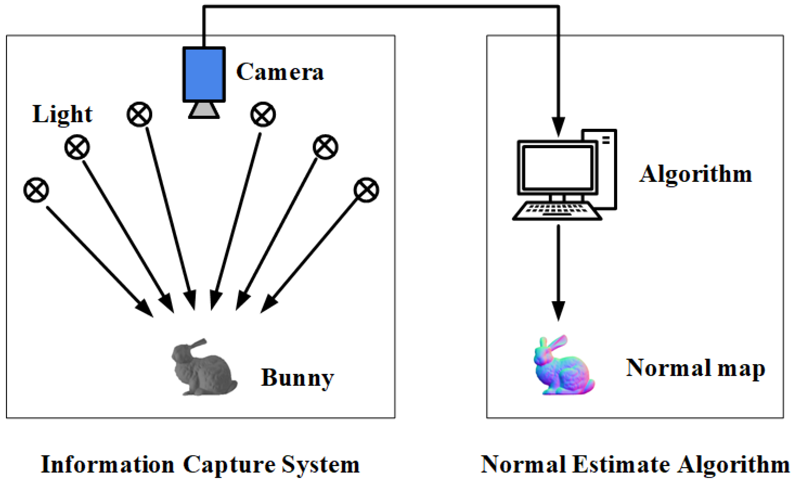
2.1. Principle of Photometric Stereo

Photometric stereo was proposed by Woodham in 1998 [12], and uses the light and shade information of the surface to analyze the light reflection model. Given images of the surface under different lighting directions with a fixed camera, the normal of the surface is calculated from the image brightness. Figure 1 shows a typical photometric stereo system, which consists of two parts: the photometric stereo information capture system and the photometric stereo normal estimate algorithm. The photometric stereo information acquisition system mainly includes a fixed camera and multiple LED lights. The camera captures a number of images when each light is sequentially turned on. The surface normal map can be solved from the acquired multiple images through the photometric stereo algorithm.
Early photometric stereo algorithms usually assumed an ideal Lambertian reflectance model [12], and the image acquisition process can be formulated as:
I = ρ max n l , 0 ,
where I represents the intensity of the captured image, ρ represents the surface albedo which is constant, n represents the surface normal which is a unit vector, l represents the lighting direction, and max n l , 0 denotes attached shadows. The normal map can be solved by Equation (1) with three or more images [12].
Unfortunately, most real-world objects are non-Lambertian. For non-Lambertian, the image forming formula can be written as [32]:
I = 0 Q ( λ ) E ( λ ) S ( λ ) d λ ,
where ( λ ) represents the spectral length, Q c ( λ ) represents spectral sensitivity of the camera, E ( λ ) represents the spectral distribution of the light, and S ( λ ) represents the spectral reflectance of the object surface.
Normally, it is difficult to directly solve the normal n through this formula. As mentioned in Section 1, many researches have been proposed to solve the problem of non-Lambertian surfaces. Our method belongs to the fourth category. We let the network directly learn the mapping between the normal map and the captured images. Our method will be discussed in detail in Section 2.2.

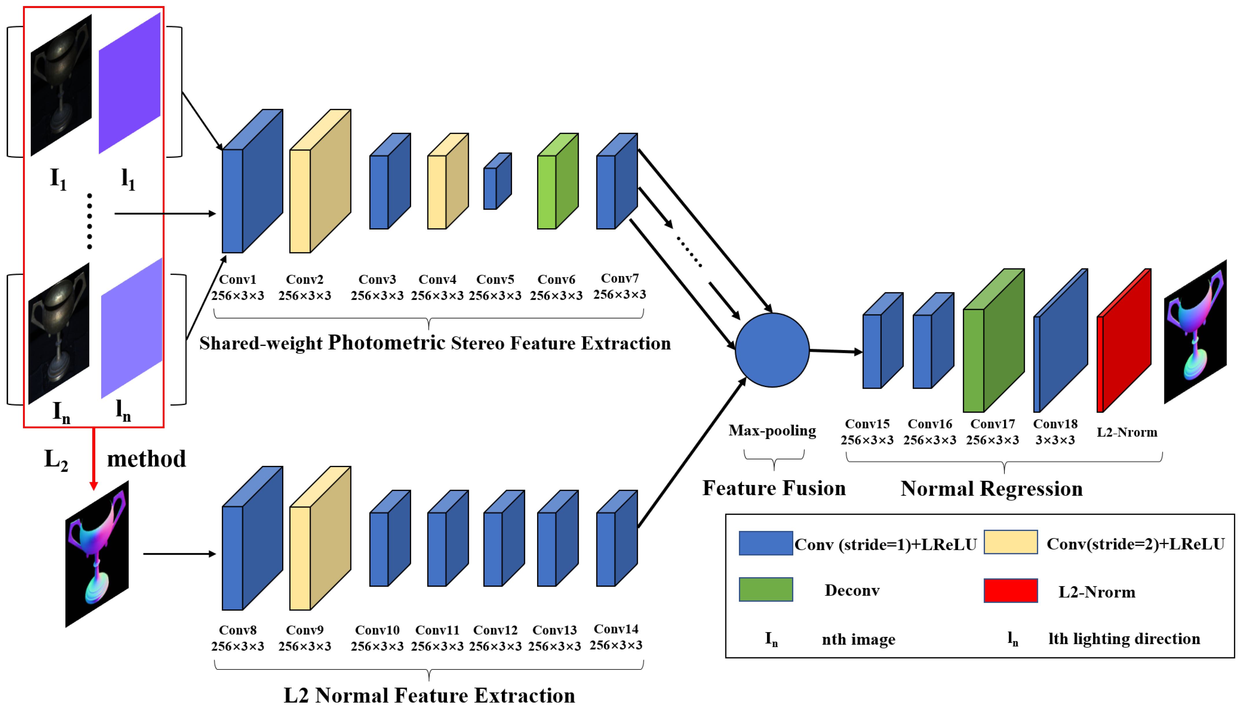
2.2. Learning Based Photometric Stereo: FFCNN

We adopt two commonly-used assumptions in photometric stereo, i.e., orthogonal cameras and directional lights. According to the semiparameter BRDF model [23,33], for most isotropic reflectances, the image formation equation of photometric stereo can be written as:
I = f B R D F n , v , l m a x ( n T l , 0 ) ,
where f B R D F represents the BRDF function, n represents the surface normal, l is the lighting direction, and v is the viewing direction, which is [ 0 , 0 , 1 ] .
For a Lambertian surface, the BRDF is a constant, and the L2 method (least square method) [12] can solve the surface normal well through three or more observations. However, the Lambertian surface barely exists. For a non-Lambertian surface, the problem of predicting normal n from the light source direction l and image brightness I is significantly more complicated because the BRDF function is unknown.
We design a learning-based approach to solve the problem of non-Lambertian. Instead of solving for n directly, we implicitly learn the mapping between input [ I , l ] and output n through the feature fusion convolutional neural network named FFCNN.
Firstly, we use a normalization strategy to process the image following [31]. Points at the same position in each image are processed as follows:
i 1 , , i m = i 1 i 1 2 + + i m 2 , , i m i 1 2 + + i m 2 ,
where i and i represent the value of original and processed points, i 1 and i m represents points in the same position on the first images and the m th images. This can remove the effect of reflectivity in low-frequency information, which is very close to Lambertian reflectance [22].
It should be noted that when the number of input images during the test time and the number of input images during the training are different, the scale of the data will be different. For example, when the pixel values of the image are all 1, the number of input images during training is q, the number of input images during training is t, and the ratio of the input value during testing to the image during training is q / t . We multiply the normalized image by a factor t / q during the test.
Meanwhile, the initial normal is calculated by the L2 method [12] as the input of the subnetwork, which can provide sufficient prior information for FFCNN network. Then we use the preprocessed images and initial normal as the input of FFCNN to estimate the accurate surface normal. It can be written as:
N = f [ I 1 , , I m ] , [ l 1 , , l m ] , N i n i t i a l ,
where f ( ) represents the FFCNN model, N represents the estimated normal map, [ I 1 , I m ] represents images from the first to the m th , [ l 1 , , l m ] represents the corresponding lighting directions, and N i n i t i a l represents normal map solved by L2 method.
As illustrated in Figure 2, our proposed FFCNN model consists of four major components including photometric stereo image feature extraction, L2 normal feature extraction, feature fusion and normal map estimation.
Given m images and m corresponding lighting directions, we expand each light direction into a lighting map with the same size as the image, and then concat the image and lighting map to obtain a 6 × H × W input image IL. Thus, we have m input matrix IL.
Then, the preprocessed data IL is fed into the network named FFCNN. We first deploy a photometric stereo feature extraction module to extract feature map F I L . All the input matrix IL are fed into the photometric stereo feature extraction network sequentially, which means they share the same weight. The shared-weight photometric stereo feature extractor module is composed of seven convolution layers with 256 channels. Downsampling is carried out at the second convolution layer and the fourth convolution layer, and up-sampling is carried out at the sixth convolution layer, which greatly increases the receptive field of the network and reduces the memory usage. Given m image-lighting data IL, m feature maps F I L are obtained by this module.
Then, we deploy an L2 normal feature extraction module to extract feature map F L 2 from the normal map solved by the L2 method [12]. Unlike the photometric stereo feature extraction module, only one down-sampling is performed at the second convolution layer in this module. The remaining 6 convolution layers are all convolution layers with 256 channels.
In the feature fusion module, m feature maps F I L and one feature map F L 2 are concatenated. Next, we apply max-pooling [29] to aggregate the features on each feature map, which means that only the maximum feature value is retained for each point. Maxpooling is widely used in photometric stereo, due to the removal of non-activated features, the influence of cast shadows can be eliminated.
Finally, a normal regression module is used to estimate the surface normal. Four convolution layers including an up-sampling convolution layer are used to achieve the same spatial dimensions as the input image. Finally, the L2-Normalization layer is used to normalize the estimated normal map.
In the FFCNN network, all convolutional layers are followed by a Leaky ReLU activation layer. Except for up-sampling layers, all convolution layers adopt kernels size with dimensions of 3 × 3 .
In the training stage, we calculate the cosine similarity error between the estimated normal and ground truth as the loss function as follows:
L = 1 H W i , j 1 N i , j · N ˜ i , j ,
where N i , j and N i , j represent the estimated normal and ground-truth, respectively. H and W are the height and width of the normal map, respectively. L is minimized using Adam with the suggested default settings. The more similar N i , j and N i , j are, the closer L is to 0.

3. Dataset and Implementation Details
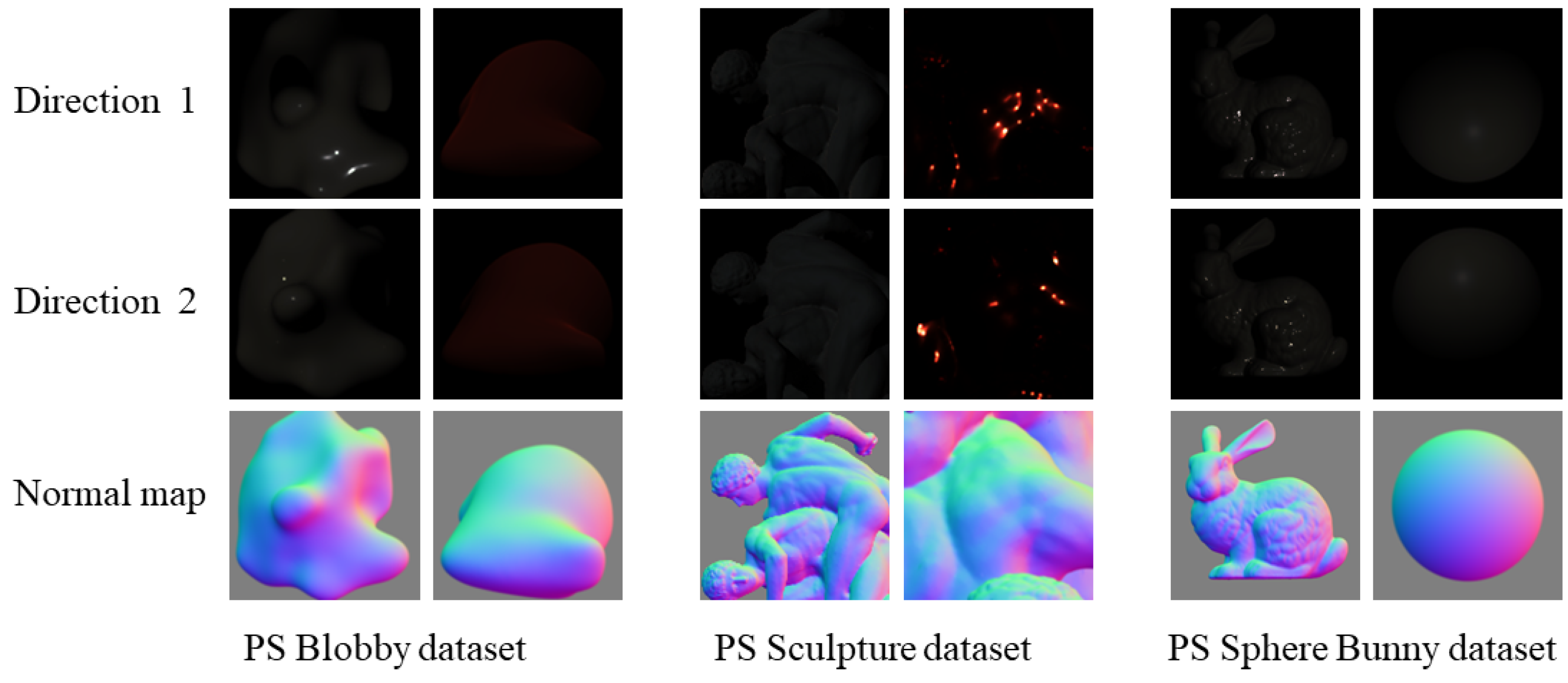
3.1. Dataset

For training and testing, ground-truth is necessary for the calculation of loss during training and evaluation during testing, and a mass of data are also needed. However, it is very difficult to get enough photometric stereo data and ground-truth. Hence, we use two publicly available synthetic datasets called the PS Blobby dataset and the PS Sculpture dataset for training and one publicly available synthetic dataset called the PS Sphere Bunny dataset for testing [29] (see Figure 3).
The MERL dataset is used for synthetic datasets to render 3D objects under different lighting conditions, which contains 100 different BRDFs of real-world materials [34]. The synthetic training datasets use two 3D datasets namely the blobby shape dataset and the sculpture shape dataset, containing 3D models of multiple objects [35,36]. The synthetic testing dataset uses 3D models of s p h e r e and b u n n y to render photometric stereo data with 100 different materials.
In addition, a publicly available real-world photometric stereo dataset called DiLi-GenT [37] is used to verify the ability of the model to process real-world data, which contains real-world data of 10 objects under 96 different lighting conditions.

3.2. Training Details

All experiments are performed in the Ubuntu operating system on a computer with GeForce RTX 3090 Graphics Card and 256GB RAM. Our FFCNN model has 9.21 million learnable parameters. During training, the initial learning rate is set to 0.001, and the learning rate is reduced to half for every 5 epochs. It takes about 8 h to train the FFCNN model when the batch size is 32 and the epoch is 30. Following [29], the height and width of the image are randomly rescaled between [ 32 , 128 ] so that the model could cope with an input of different sizes, and the image is then randomly cropped to 32 × 32 and noise is randomly added.

3.3. Testing Details

The PS Sphere Bunny dataset is used to illustrate the ability of the FFCNN model to estimate normal maps on the synthetic dataset. The DiLiGenT benchmark dataset is used to verify the generalization ability of the FFCNN model in dealing with real-world photometric stereo data. The accuracy of the normal estimation is quantitatively evaluated by the average angular error (MAE) between the ground-truth normal map and the estimated normal map as:
M A E = arccos 1 K k 1 n k · n ˜ k ,
where n k and n ˜ k represent the ground-truth and the predicted normal maps, respectively. K represents the number of all pixels in the image except the background area. A lower MAE means a more accurate normal map estimated by the model. The photometric stereo data of the polished rail surface are used to verify the generalization of the model and qualitative analysis of the effect of the model in the industrial field.

4. Experiments and Results

4.1. Network Analysis

4.1.1. Effects of Kernel Size

The kernel size affects the receptive field of FFCNN, thus affecting the performance of the network. For each point, the larger the kernel size is, the more information from neighboring points can be used to estimate the normal of the point. However, if the point is too far away from the estimated point, it will have less useful information for the estimated point, and may even contain interfering information. Besides, it will also increase the computational complexity and time cost. We use the PS Sphere Bunny dataset to compare the performance of our model with different kernel sizes. The number of input images is 32 during training and 100 during testing. Both Sphere and Bunny contain data for 100 materials, and the result for each material is the average of 100 random trails. We take the average of the results for all materials. Figure 4 presents the relationship between the kernel size and the MAE of normal estimation.
As illustrated in Figure 4, the MAE does not decrease continuously as the kernel size increases. On both b u n n y and s p h e r e datasets, MAE decreases as the kernel size increases until the kernel size increases to 3. However, when the kernel size increases to 5 and 7, the MAE keeps increasing. This verifies our conjecture that when the kernel size is too large, the point too far from the estimated point may contain redundant information that interferes with the normal estimation. To achieve the best performance, we empirically set the kernel size to 3.

4.1.2. Effects of Input Number

The number of input images during training will also affect the performance of the model. Table 1 lists the performance of FFCNN model with different numbers of input images during training and testing.
For a fixed number of inputs during training, the performance of FFCNN basically increases with the number of inputs during testing. When the number of input images during testing is fixed and fewer than 32, FFCNN performs better when the number of input images during training is 2 times that during testing. When the number of input images during testing is fixed and not less than 32, FFCNN performs slightly better when the number of input images is 32 during training. Considering the performance of FFCNN for estimating the normal and the memory of the computer, we use 32 images during training.

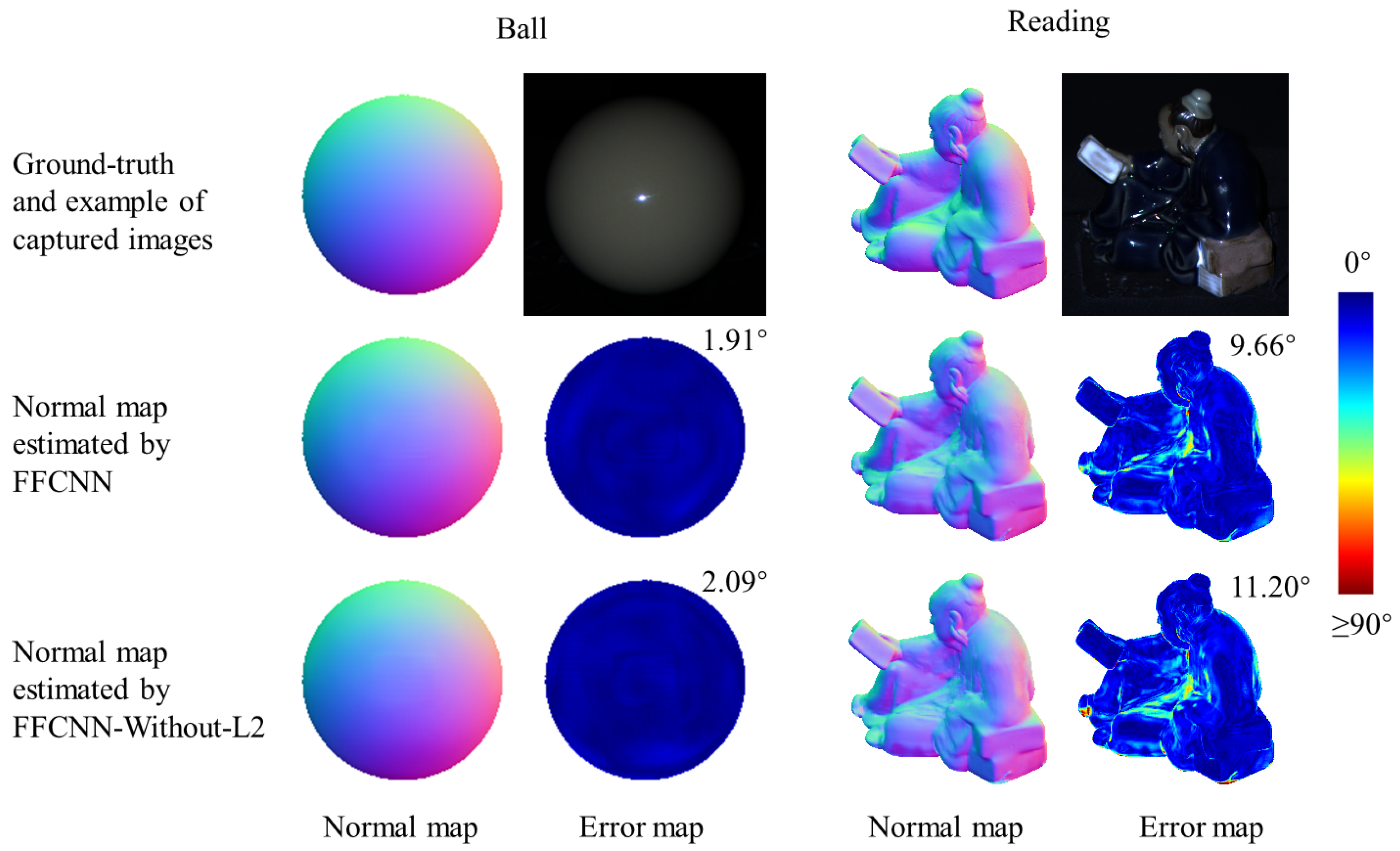
4.1.3. Effects of Feature Fusion

The L2 method performs poorly for non-Lambertian surfaces, especially for specular reflection. However, the low frequency information in the image is very close to Lambertian reflection, and the L2 method can estimate the normal map of this part well. The initial normal obtained by L2 method provides useful prior information for FFCNN to extract normal features from observation images. For specular reflection, the normal vector can be regarded as the bisector of the viewing and light directions. The max-pooling operation can extract these significant features and ignore the non-activated features of cast shadow.
Table 2 shows the comparison of the performance of FFCNN and FFCNN-Without-L2. FFCNN-Without-L2 is the same as FFCNN but without the L2 normal feature extraction module. As shown in Table 2, on both b u n n y and s p h e r e , FFCNN performs better than FFCNN-Without-L2. On the real-world object DiLiGenT benchmark dataset, FFCNN performs significantly better than FFCNN-Without-L2 in terms of the average of MAE on ten objects. The performance of FFCNN is obviously superior in most objects, and it is inferior to FFCNN-Without-L2 in only three objects, but the difference is very small. This means that our proposed feature fusion strategy is effective, especially on objects with complex structures, such as the r e a d i n g object.
Figure 5 shows the comparison of the performance of FFCNN and FFCNN-Without-L2 on two objects, b a l l and r e a d i n g . It can be seen from the b a l l object that the performance of FFCNN is better than that of FFCNN-Without-L2 in the non-specular reflection area, which also verifies our conjecture that the L2 method can estimate the normal map close to the Lambertian region well, which provides prior information for FFCNN. Our feature fusion method also performs well on the r e a d i n g object with more complex surfaces and more specular reflection areas.

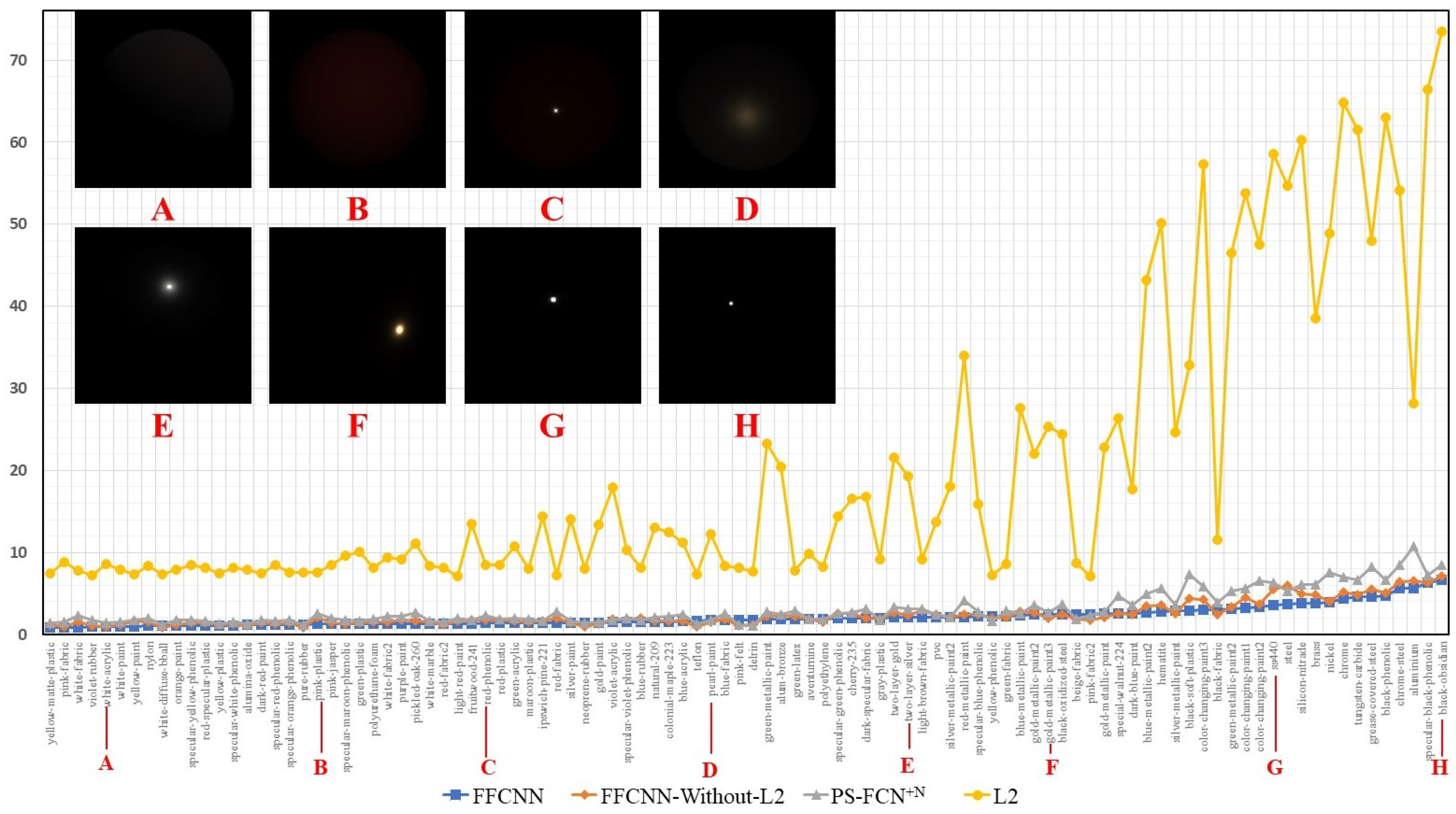
4.1.4. Results on Different Materials

Specular reflection is a challenging problem in photometric stereo. The surface of many materials has specular reflection characteristics, especially in the industrial field. Figure 6 compares FFCNN with L2 Baseline [12], PS-FCN+N [31] and FFCNN-Without-L2 on samples of s p h e r e object that were rendered with 100 different BRDFs, which contain a large number of materials with specular reflective properties.
In Figure 6, the performance of FFCNN represented by the blue line is significantly better than the other three methods. The material represented on the right of the horizontal axis in this figure contains more intense specular reflection, and our method performs better on these materials, indicating that our method can handle specular reflection surfaces well.

4.2. Benchmark Comparisons

4.2.1. Quantitative Comparison

We compare our method FFCNN with several other state-of-the-art photometric stere solutions including IA-14 [23], ST-14 [22], HI-17 [27], TM-18 [38], CH-18 [29], SI-18 [28], CA-21 [30], and CH-20 [31]. The source code and evaluation results for these methods are publicly available. All 96 images are used to estimate the normal direction of the object. The MAE of the normal map estimated by these methods on the DiLiGenT benchmark dataset is shown in Table 3.
Our proposed FFCNN model achieved the best results on 10 real-world objects, with a mean angle error of 6.83 . For objects with strong specular reflection or complex geometric surfaces, such as r e a d i n g and c o w objects, our model performs significantly better than other methods. This illustrates that the proposed network can effectively deal with specular reflection or complex geometric surfaces.
Please note that it was considered that the first 20 images of the b e a r object were corrupted in SI-18 [28]. After discarding the first 20 images of the b e a r object, we compare our method FFCNN with the method termed CNN-PS in SI-18 [28], as shown in Table 4. Although our proposed method is slightly inferior to CNN-PS on the b e a r object, the overall performance of our method on 10 objects is still significantly better.
Table 5 compares the proposed FFCNN and CNN-PS in SI-18 [28] in terms of running time. We repeat the estimation process 10 times and compute the average running time (the forward time of the network). Following the setting in SI-18 [28], we set the number of different rotations for the rotational pseudo-invariance to 10. Since CNN-PS estimates the normal map in a pixel-wise manner, while our method estimates the normal map in a frame-wise manner, the running time of CNN-PS is much more than that of FFCNN. Therefore, our proposed FFCNN is more suitable for applications in industrial fields where high efficiency is required.

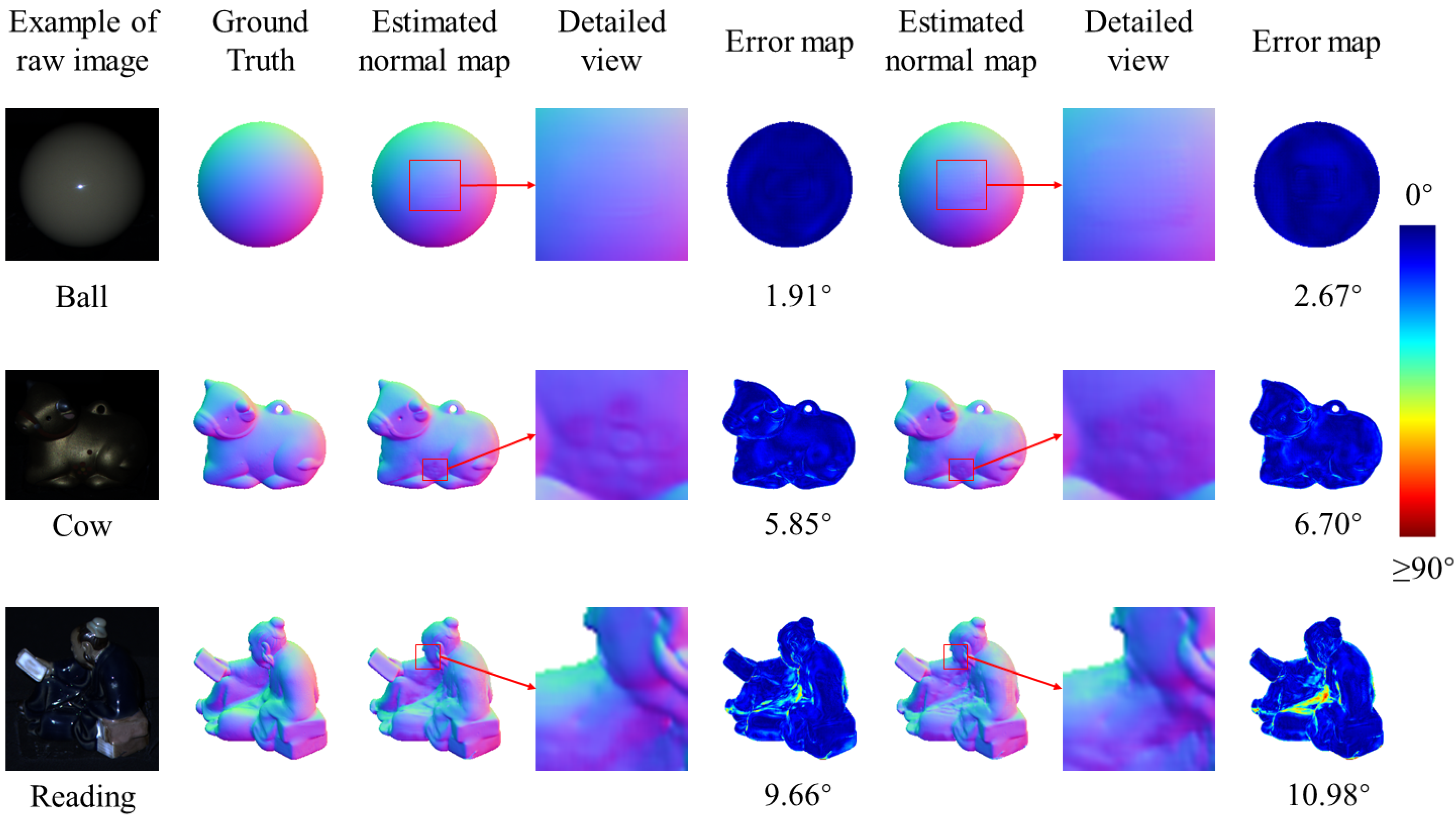
4.2.2. Qualitative Comparison

Figure 7 shows some qualitative results on three real-world objects in the DiLiGenT benchmark dataset. For the object b a l l , we use 96 images to estimate the normal map, which means there will be 96 highlight areas. It can be seen from the estimated normal map and the detailed view that our method can handle the specular reflection problem well and estimate a more accurate normal map. For c o w and r e a d i n g objects, it can be seen in the detail view and the error map that our proposed FFCNN model is capable of estimating the normal map with richer details.

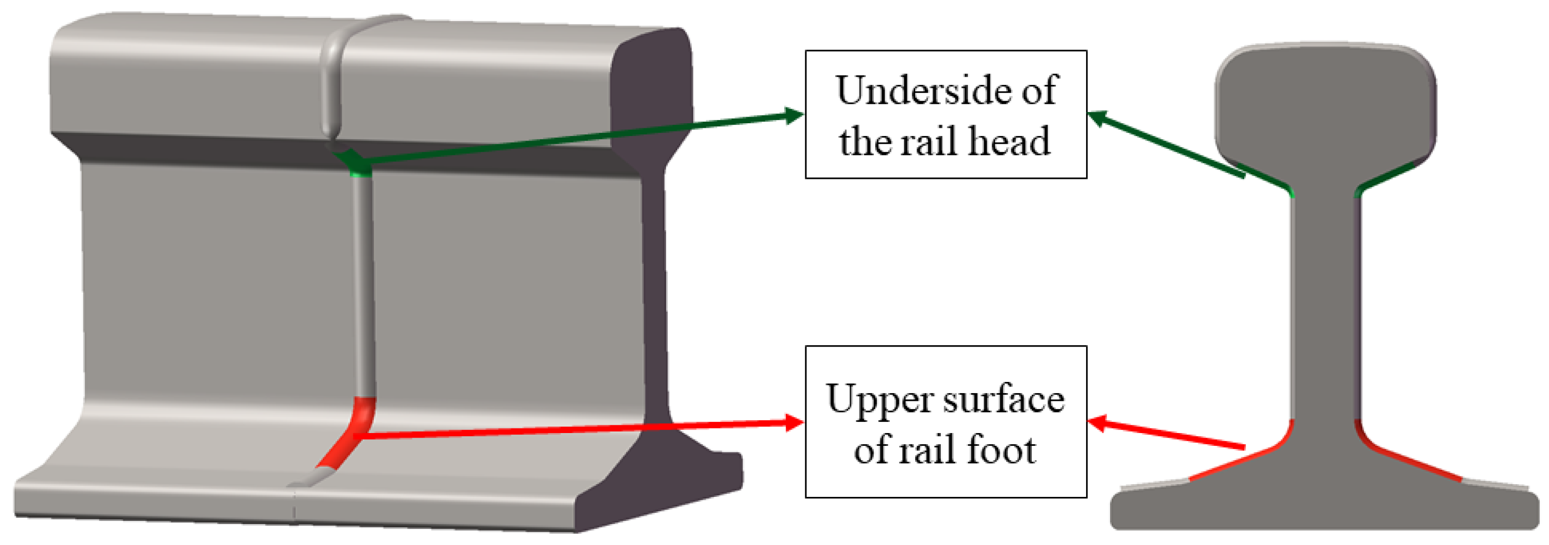
4.3. Application in Industrial Field

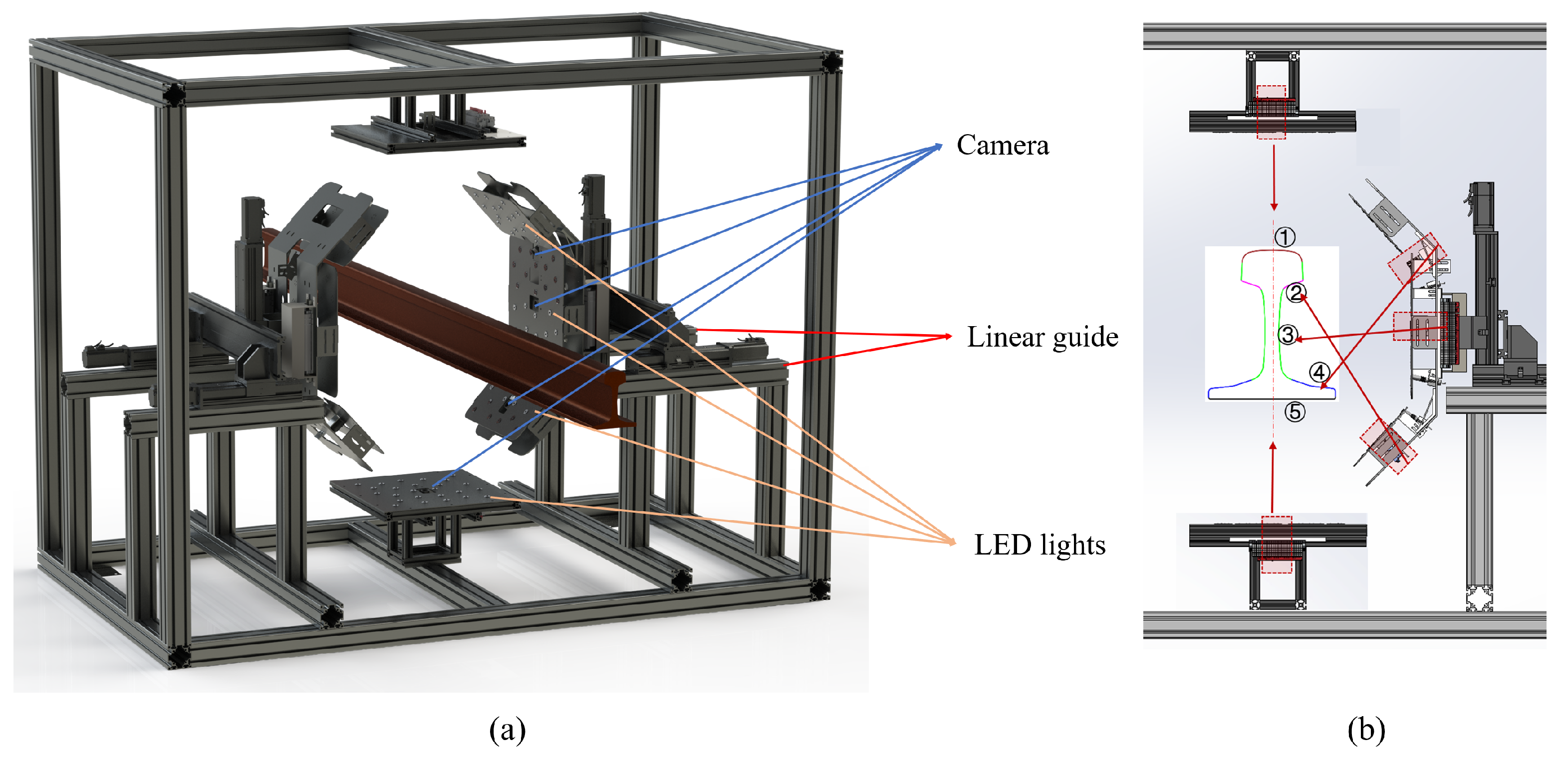
4.3.1. The Setup of Photometric Stereo System

To validate the effectiveness of our FFCNN model in industry, we apply FFCNN to normal map estimation of the polished rail welding surface, which contains severe specular reflections and complex reflection characteristics. Obtaining information of the product surface is the first step in applying photometric stereo to industrial applications. However, the geometric surface of the rail is complicated, the underside of the rail head and the upper surface of the rail foot are difficult to be illuminated by multiple light sources as well as reflected to the camera. Figure 8 is an illustration of the problem. Because of the special geometry of the rail, the information gathering of the red and green marked areas is challenging.
Therefore, we design a novel photometric stereo image data capture system to solve this problem, as shown in Figure 9. The system consists of four parts, two identical surface information acquisition systems are used to obtain information on the top surface of the rail and information on the bottom surface of the rail namely IASa and IASb (IAS* represents image acquisition system), two identical and symmetrical information acquisition module to obtain information of the rail waist namely IASc and IASd. The module IASa or IASb are composed of a fixed orientation camera and a number of LED lights around the camera. The module IASc or IASd consists of three cameras and LED lights around the camera. The upper and lower cameras in the module IASc or IASd are oriented towards the underside of the rail head and the upper surface of the rail foot respectively to capture information on the concave surfaces. The middle camera is perpendicular to the waist of the rail. In addition, there is a two-degree-of-freedom guide rail on the side for the module IASc or IASd to adjust the height of the module and the distance between the rail and the module. The structure made of profiles supports the operation of the whole equipment. We designed a circuit to control the collaboration between the LED lights and the camera. We used Raspberry PI to send signals which control relays to switch each LED light on and off individually, and the camera takes an image when the LED is turned on. A 5V constant voltage power supply powers the Raspberry PI, and a 700 mA constant current power supply keeps the brightness of each LED light constant, as the surface normal can only be solved by keeping the brightness of the LED lights constant.
With this equipment, we can collect information of the welded rail surface after grinding from multiple perspectives.

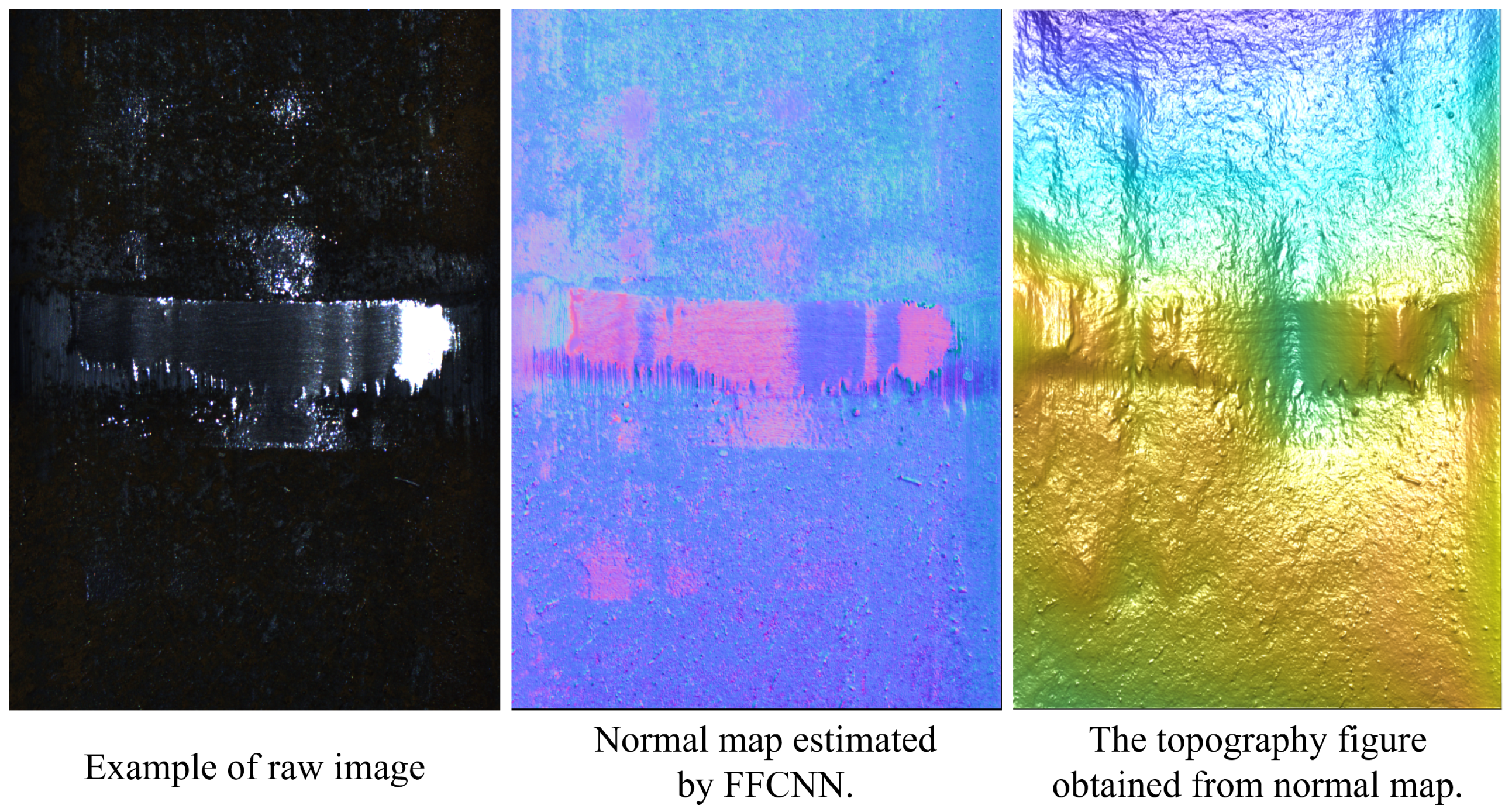
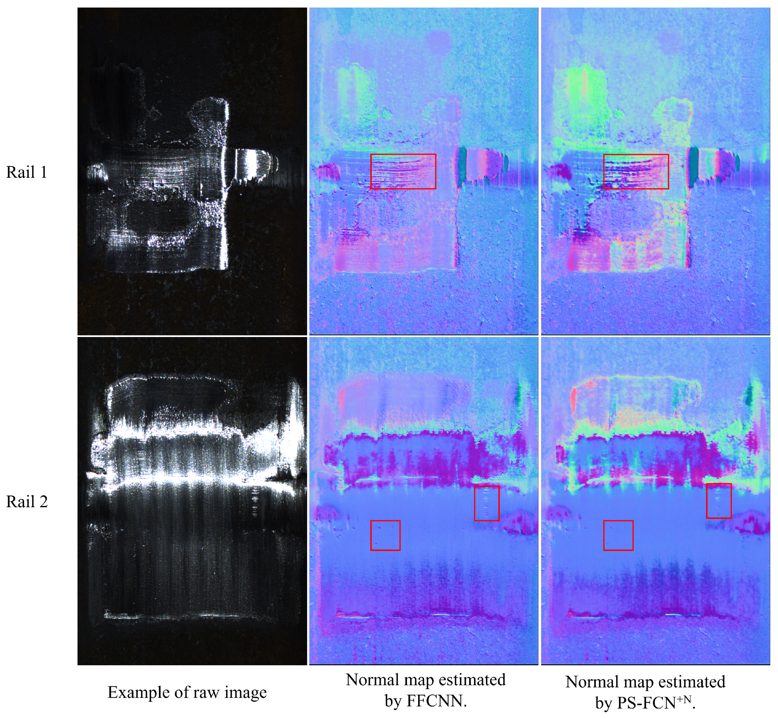
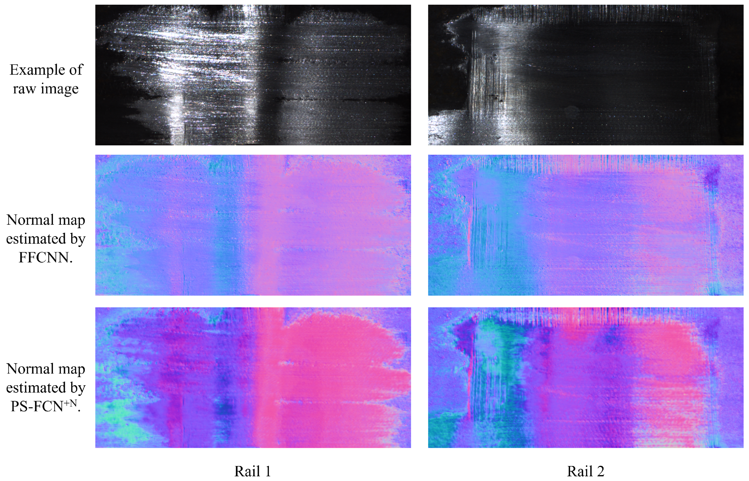
4.3.2. Result on Polished Rail Welding Surface

After obtaining the surface information of the polished rail, we use our proposed FFCNN to estimate the normal map. Some examples of results on the top surface of the rail, the waist of the rail and the upper surface of the rail foot are shown in Figure 10, Figure 11, and Figure 12, respectively.
As shown in Figure 10, the normal map estimated by our method contains rich detailed information, although the acquired image contains a large area of specular reflection. Figure 11 compares the performance of FFCNN and PS-FCN+N [31] on two samples of rail waist respectively. FFCNN performs significantly better than PS-FCN+N, especially in detailed information, as shown in the red box marked area. The normal map estimated by FCCNN contains more detailed information, while the important details in the normal map estimated by PS-FCN+N are smoothed. Figure 12 compares the performance of FFCNN and PS-FCN+N on two samples of the upper surface of the rail foot, respectively. Similarly, FFCNN performs significantly better than PS-FCN+N, and the estimated normal map of PS-FCN+N seems to be wrong. The normal map estimated by FFCNN performs well in terms of details and textures, which can provide rich information for the subsequent detection and evaluation of polishing quality, as shown in the red box in Figure 11.

5. Conclusions

In this paper, we propose a complete photometric stereo processing framework to estimate the normal map of non-Lambertian surfaces, especially polished surfaces. We propose a feature fusion neural network to regress the surface normal map, which uses the initial normal map obtained by the L2 method as prior information, and fuses the features extracted from the original image with the features extracted from the initial normal map. The proposed method makes full use of the low-frequency information close to the Lambertian and the information of the specular reflection area to make the estimated normal map more accurate. We have experimentally investigated and verified the performance of our model. The proposed method performs better than the state-of-the-art methods on both synthetic datasets and real-world object DiLiGenT benchmark dataset. Additionally, the proposed method is used to estimate the normal map of the polished rail welding surface, verifying the effectiveness of our method in the industrial field. We design a photometric stereo information capture system with multi-view cameras and multi-angle lights to obtain the surface information of polished rail welding surface with complex geometric surfaces. The normal map of the polished rail welding surface estimated by our FFCNN model contains rich texture information and detailed information, which can provide rich information for surface quality evaluation. This demonstrates the effectiveness of our method for industrial non-Lambertian surfaces, as well as specular reflective surfaces.

Author Contributions

Conceptualization, Y.C. (Yanlong Cao) and X.W.; Data curation, Y.C. (Yanpeng Cao); Formal analysis, J.Y.; Funding acquisition, Y.C. (Yanlong Cao); Investigation, Y.C. (Yanlong Cao); Methodology, Y.C. (Yanlong Cao) and X.W.; Project administration, Y.C. (Yanlong Cao); Resources, Y.C. (Yanpeng Cao); Software, X.W. and W.L. Supervision, J.Y. and Y.C. (Yanpeng Cao); Validation, X.W., W.L. and B.D.; Visualization, X.W.; Writing—original draft, X.W. and Y.C. (Yanpeng Cao); Writing—review & editing, X.W. and B.D. All authors have read and agreed to the published version of the manuscript.

Funding

This research was funded by National Natural Science Foundation of China, grant number 52175520.

Institutional Review Board Statement

Not applicable.

Informed Consent Statement

Not applicable.

Data Availability Statement

The data presented in this study are available on request from the correspondingauthor. The data are not publicly available due to the privacy policy of the organization.

Acknowledgments

The authors gratefully acknowledge China Railway Jinan Group Co Ltd. for providing the rails and the experimental site.

Conflicts of Interest

The authors declare no conflict of interest.

References

  1. Cui, Z.; Lu, W.; Liu, J. Real-time industrial vision system for automatic product surface inspection. In Proceedings of the 2016 8th International Conference on Information Management and Engineering, Istanbul, Turkey, 2–5 November 2016; pp. 93–97. [Google Scholar]
  2. Zheng, X.; Zheng, S.; Kong, Y.; Chen, J. Recent advances in surface defect inspection of industrial products using deep learning techniques. Int. J. Adv. Manuf. Technol. 2021, 113, 35–58. [Google Scholar] [CrossRef]
  3. Chen, Y.; Ding, Y.; Zhao, F.; Zhang, E.; Wu, Z.; Shao, L. Surface Defect Detection Methods for Industrial Products: A Review. Appl. Sci. 2021, 11, 7657. [Google Scholar] [CrossRef]
  4. Kowal, J.; Sioma, A. Surface defects detection using a 3D vision system. In Proceedings of the 13th International Carpathian Control Conference (ICCC), High Tatras, Slovakia, 28–31 May 2012; pp. 382–387. [Google Scholar]
  5. Yan, Z.; Shi, B.; Sun, L.; Xiao, J. Surface defect detection of aluminum alloy welds with 3D depth image and 2D gray image. Int. J. Adv. Manuf. Technol. 2020, 110, 741–752. [Google Scholar] [CrossRef]
  6. Rosati, G.; Boschetti, G.; Biondi, A.; Rossi, A. Real-time defect detection on highly reflective curved surfaces. Opt. Lasers Eng. 2009, 47, 379–384. [Google Scholar] [CrossRef]
  7. Tang, Y.; Wang, Q.; Wang, H.; Li, J.; Ke, Y. A novel 3D laser scanning defect detection and measurement approach for automated fibre placement. Meas. Sci. Technol. 2021, 32, 075201. [Google Scholar] [CrossRef]
  8. Cao, X.; Xie, W.; Ahmed, S.M.; Li, C.R. Defect detection method for rail surface based on line-structured light. Measurement 2020, 159, 107771. [Google Scholar] [CrossRef]
  9. Zhang, S. High-speed 3D shape measurement with structured light methods: A review. Opt. Lasers Eng. 2018, 106, 119–131. [Google Scholar] [CrossRef]
  10. Lee, J.H.; Oh, H.M.; Kim, M.Y. Deep learning based 3D defect detection system using photometric stereo illumination. In Proceedings of the 2019 International Conference on Artificial Intelligence in Information and Communication (ICAIIC), Okinawa, Japan, 11–13 February 2019; pp. 484–487. [Google Scholar]
  11. Kang, D.; Jang, Y.J.; Won, S. Development of an inspection system for planar steel surface using multispectral photometric stereo. Opt. Eng. 2013, 52, 039701. [Google Scholar] [CrossRef] [Green Version]
  12. Woodham, R.J. Photometric method for determining surface orientation from multiple images. Opt. Eng. 1980, 19, 191139. [Google Scholar] [CrossRef]
  13. Wu, L.; Ganesh, A.; Shi, B.; Matsushita, Y.; Wang, Y.; Ma, Y. Robust photometric stereo via low-rank matrix completion and recovery. In Proceedings of the Asian Conference on Computer Vision; Springer: Berlin/Heidelberg, Germany, 2010; pp. 703–717. [Google Scholar]
  14. Mukaigawa, Y.; Ishii, Y.; Shakunaga, T. Analysis of photometric factors based on photometric linearization. JOSA A 2007, 24, 3326–3334. [Google Scholar] [CrossRef]
  15. Miyazaki, D.; Hara, K.; Ikeuchi, K. Median photometric stereo as applied to the segonko tumulus and museum objects. Int. J. Comput. Vis. 2010, 86, 229. [Google Scholar] [CrossRef]
  16. Wu, T.P.; Tang, C.K. Photometric stereo via expectation maximization. IEEE Trans. Pattern Anal. Mach. Intell. 2009, 32, 546–560. [Google Scholar]
  17. Ikehata, S.; Wipf, D.; Matsushita, Y.; Aizawa, K. Robust photometric stereo using sparse regression. In Proceedings of the 2012 IEEE Conference on Computer Vision and Pattern Recognition, Providence, RI, USA, 16–21 June 2012; pp. 318–325. [Google Scholar]
  18. Tozza, S.; Mecca, R.; Duocastella, M.; Del Bue, A. Direct differential photometric stereo shape recovery of diffuse and specular surfaces. J. Math. Imaging Vis. 2016, 56, 57–76. [Google Scholar] [CrossRef] [Green Version]
  19. Georghiades, A.S. Incorporating the torrance and sparrow model of reflectance in uncalibrated photometric stereo. In Proceedings of the IEEE International Conference on Computer Vision, Nice, France, 13–16 October 2003; Volume 3, p. 816. [Google Scholar]
  20. Chung, H.S.; Jia, J. Efficient photometric stereo on glossy surfaces with wide specular lobes. In Proceedings of the 2008 IEEE Conference on Computer Vision and Pattern Recognition, Anchorage, AK, USA, 23–28 June 2008; pp. 1–8. [Google Scholar]
  21. Ruiters, R.; Klein, R. Heightfield and spatially varying BRDF reconstruction for materials with interreflections. Comput. Graph. Forum 2009, 28, 513–522. [Google Scholar] [CrossRef]
  22. Shi, B.; Tan, P.; Matsushita, Y.; Ikeuchi, K. Bi-Polynomial Modeling of Low-Frequency Reflectances. IEEE Trans. Pattern Anal. Mach. Intell. 2014, 36, 1078–1091. [Google Scholar] [CrossRef]
  23. Ikehata, S.; Aizawa, K. Photometric stereo using constrained bivariate regression for general isotropic surfaces. In Proceedings of the IEEE Conference on Computer Vision and Pattern Recognition, Columbus, OH, USA, 23–28 June 2014; pp. 2179–2186. [Google Scholar]
  24. Holroyd, M.; Lawrence, J.; Humphreys, G.; Zickler, T. A photometric approach for estimating normals and tangents. ACM Trans. Graph. 2008, 27, 1–9. [Google Scholar] [CrossRef]
  25. Hertzmann, A.; Seitz, S.M. Example-based photometric stereo: Shape reconstruction with general, varying brdfs. IEEE Trans. Pattern Anal. Mach. Intell. 2005, 27, 1254–1264. [Google Scholar] [CrossRef]
  26. Hui, Z.; Sankaranarayanan, A.C. A dictionary-based approach for estimating shape and spatially-varying reflectance. In Proceedings of the 2015 IEEE International Conference on Computational Photography (ICCP), Houston, TX, USA, 24–26 April 2015; pp. 1–9. [Google Scholar]
  27. Santo, H.; Samejima, M.; Sugano, Y.; Shi, B.; Matsushita, Y. Deep photometric stereo network. In Proceedings of the IEEE International Conference on Computer Vision Workshops, Venice, Italy, 22–29 October 2017; pp. 501–509. [Google Scholar]
  28. Ikehata, S. CNN-PS: CNN-based photometric stereo for general non-convex surfaces. In Proceedings of the European Conference on Computer Vision (ECCV), Munich, Germany, 8–14 September 2018; pp. 3–18. [Google Scholar]
  29. Chen, G.; Han, K.; Wong, K.Y.K. PS-FCN: A flexible learning framework for photometric stereo. In Proceedings of the European Conference on Computer Vision (ECCV), Munich, Germany, 8–14 September 2018; pp. 3–18. [Google Scholar]
  30. Cao, Y.; Ding, B.; He, Z.; Yang, J.; Chen, J.; Cao, Y.; Li, X. Learning inter-and intraframe representations for non-Lambertian photometric stereo. Opt. Lasers Eng. 2022, 150, 106838. [Google Scholar] [CrossRef]
  31. Chen, G.; Han, K.; Shi, B.; Matsushita, Y.; Wong, K.Y.K. Deep photometric stereo for non-Lambertian surfaces. IEEE Trans. Pattern Anal. Mach. Intell. 2020, 44, 129–142. [Google Scholar] [CrossRef]
  32. Miyazaki, D.; Onishi, Y.; Hiura, S. Color photometric stereo using multi-band camera constrained by median filter and occluding boundary. J. Imaging 2019, 5, 64. [Google Scholar] [CrossRef] [Green Version]
  33. Chandraker, M.; Ramamoorthi, R. What an image reveals about material reflectance. In Proceedings of the 2011 International Conference on Computer Vision, Barcelona, Spain, 6–13 November 2011; pp. 1076–1083. [Google Scholar]
  34. Matusik, W.; Pfister, H.; Brand, M.; McMillan, L. A Data-Driven Reflectance Model. ACM Trans. Graph. 2003, 22, 759–769. [Google Scholar] [CrossRef]
  35. Johnson, M.K.; Adelson, E.H. Shape estimation in natural illumination. In Proceedings of the CVPR 2011, Colorado Springs, CO, USA, 20–25 June 2011; pp. 2553–2560. [Google Scholar]
  36. Zisserman, A.; Wiles, O. SilNet: Single-and Multi-View Reconstruction by Learning from Silhouettes; Oxford University: Oxford, UK, 2017. [Google Scholar]
  37. Shi, B.; Wu, Z.; Mo, Z.; Duan, D.; Yeung, S.K.; Tan, P. A benchmark dataset and evaluation for non-lambertian and uncalibrated photometric stereo. In Proceedings of the IEEE Conference on Computer Vision and Pattern Recognition, Las Vegas, NV, USA, 27–30 June 2016; pp. 3707–3716. [Google Scholar]
  38. Taniai, T.; Maehara, T. Neural inverse rendering for general reflectance photometric stereo. In Proceedings of the International Conference on Machine Learning, PMLR, Stockholm, Sweden, 10–15 July 2018; pp. 4857–4866. [Google Scholar]
Figure 1. A typical photometric stereo system containing two parts: the photometric stereo information capture system and the photometric stereo normal estimate algorithm.
Machines 10 00120 g001
Figure 2. Network architecture of FFCNN.
Machines 10 00120 g002
Figure 3. Examples of the synthetic data. The first two lines show the images of the same object under two different lighting directions, and the last line shows the normal map.
Machines 10 00120 g003
Figure 4. Effects of kernel size. The horizontal axis represents the kernel size, the vertical axis represents the average angular error (MAE), the blue line represents the performance on the b u n n y object, and the yellow line represents the performance on the s p h e r e object.
Machines 10 00120 g004
Figure 5. Comparison of FFCNN and FFCNN-Without-L2 on two objects, b a l l and r e a d i n g . The first row shows the true values and a sample of observations. The second row shows the normal and error maps estimated by the FFCNN method. The third row is the normal and error maps estimated by the FFCNN-Without-L2 method.
Machines 10 00120 g005
Figure 6. Quantitative comparison of FFCNN and FFCNN with L2 Baseline [12], PS-FCN+N [31] and FFCNN_without_L2. The horizontal axis from left to right represents the properties of the material from diffuse reflection to specular reflection. Images in the upper-left corner show the corresponding samples. Images AH correspond to samples of the material marked in the horizontal coordinates.
Machines 10 00120 g006
Figure 7. Qualitative comparison between proposed method FFCNN and the state-of-the-art method PS-FCN+N [31] on three objects, b a l l , c o w , and r e a d i n g . The detailed view contains rich texture information.
Machines 10 00120 g007
Figure 8. Appearance of the rail. The red and green marked areas contains cast shadows.
Machines 10 00120 g008
Figure 9. Illustration of the equipment. (a) Overall illustration of the equipment. It mainly contains four information acquisition systems (IASa, IASb, IASc, IASd) and two linear guides and profiles. (b) Each camera corresponds to a range of shots.
Machines 10 00120 g009
Figure 10. The normal map of upper surface of the rail estimated by FFCNN and the corresponding topographic map. The color of the topographic map represents the height of the surface.
Machines 10 00120 g010
Figure 11. The comparison of different methods on the welded surface of the rail waist after grinding. The region marked by the red box contains defects.
Machines 10 00120 g011
Figure 12. The comparison of different methods on the upper surface of the welded rail foot after grinding.
Machines 10 00120 g012
Table 1. Effects of input number. (a) Performance on b u n n y object of 100 materials. (b) Performance on s p h e r e object of 100 materials. benchmark dataset. The red values illustrate the best performance. The smaller the value of MAE means the better the model performs.
(a) Performance on bunny (MAE)
VariantsTest with # images
Train with # images4816324864100
419.8814.3310.18.197.998.098.38
816.9510.936.795.084.824.824.93
1617.409.595.363.773.493.443.50
3220.549.314.933.342.982.92.86
4822.019.545.023.443.012.92.86
(b) Performance on sphere (MAE)
VariantsTest with # images
Train with # images4816324864100
414.1610.767.595.75.445.385.56
813.819.205.113.653.473.513.82
1615.158.244.212.782.552.552.73
3217.708.253.842.392.132.072.14
4819.178.624.112.552.232.152.17
Table 2. Effects of feature fusion. (a) Performance on synthetic data PS Sphere Bunny dataset. The MAE is the calculated average value of performance on 100 materials. (b) Performance on the real-world object data DiLiGenT benchmark dataset. The red values illustrate the best performance. The smaller the value of MAE means the better the model performs.
(a) Performance on the PS Sphere Bunny dataset
modelbunnysphereaverage
FFCNN-Without-L23.232.402.81
FFCNN2.862.142.5
(b) Performance on the DiLiGenT benchmark dataset
Methodballcatpot1bearpot2buddhagobletreadingcowharvestaverage
FFCNN-Without-L22.094.665.666.737.427.347.7511.26.4612.487.18
FFCNN1.914.875.416.56.627.57.799.665.8512.226.83
Table 3. Quantitative comparison of our proposed FFCNN model and state-of-the-art photometric stereo methods on the DiLiGenT benchmark dataset. * indicates that we use all 96 images to estimate the normal map of B e a r , but the result shown in SI-18 [28] ( B e a r 4.1) was achieved by discarding the first 20 input images. The red values illustrate the best performance. The smaller the value of MAE means the better the model performs.
MethodBallCatpot1Bearpot2BuddhaGobletReadingCowHarvestAvg.
proposed1.914.875.416.506.627.507.799.665.8512.226.83
CH-20 [31]2.674.746.167.727.157.567.8810.986.7012.427.40
CA-21 [30]2.295.876.925.796.896.857.8811.947.4813.717.56
SI-18 * [28]2.204.605.4012.306.007.907.3012.607.9013.908.01
CH-18 [29]2.826.167.137.557.257.918.6013.337.3315.858.39
TM-18 [38]1.475.446.095.797.7610.3611.4711.036.3222.598.83
HI-17 [27]2.026.547.056.317.8612.6811.2815.518.0116.869.41
ST-14 [22]1.746.126.516.128.7810.6010.0913.6313.9325.4410.30
IA-14 [23]3.346.746.647.118.7710.479.7114.1913.0525.9510.60
L2 Baseline [12]4.108.418.898.3914.6514.9218.5019.8025.6030.6215.39
Table 4. Quantitative comparison of our proposed FFCNN model and CNN-PS on the DiLiGenT benchmark dataset with the first 20 images of the b e a r object discarded. The smaller the value of MAE means the better the model performs.
MethodBallCatpot1Bearpot2BuddhaGobletReadingCowHarvestAvg.
proposed1.914.875.414.526.627.507.799.665.8512.226.64
SI-18 [28]2.204.605.404.106.007.907.3012.607.9013.907.19
Table 5. Comparison of the running time of our proposed FFCNN model and CNN-PS on the corpped DiLiGenT benchmark dataset.
MethodRunning Time (s)
BallCatpot1Bearpot2BuddhaGobletReadingCowHarvestAvg.
proposed1.1990.5080.5450.3570.3830.3780.4920.2940.2680.4850.491
SI-18 [28]9.85825.60832.55523.63114.07025.41410.43011.08710.56332.26319.548
Publisher’s Note: MDPI stays neutral with regard to jurisdictional claims in published maps and institutional affiliations.

