Article

A Novel Combination Neural Network Based on ConvLSTM-Transformer for Bearing Remaining Useful Life Prediction

1
School of Mechanical Engineering, Shijiazhuang Tiedao University, Shijiazhuang 050043, China
2
State Key Laboratory of Mechanical Behavior and System Safety of Traffic Engineering Structures, Shijiazhuang Tiedao University, Shijiazhuang 050043, China
*
Authors to whom correspondence should be addressed.
Machines 2022, 10(12), 1226; https://doi.org/10.3390/machines10121226
Submission received: 5 November 2022 / Revised: 28 November 2022 / Accepted: 2 December 2022 / Published: 15 December 2022
(This article belongs to the Section Machines Testing and Maintenance)

Abstract

:
A sensible maintenance strategy must take into account the remaining usable life (RUL) estimation to maximize equipment utilization and avoid costly unexpected breakdowns. In view of some inherent drawbacks of traditional CNN and LSTM-based RUL prognostics models, a novel combination model of the ConvLSTM and the Transformer, which is based on the idea of “Extracting spatiotemporal features and applying them to RUL prediction”, is proposed for RUL prediction. The ConvLSTM network can directly extract low-dimensional spatiotemporal features from long-time degradation signals. The Transformer, based entirely on attention mechanisms, can deeply explore the mapping law between deep-level nonlinear spatiotemporal feature information and equipment service performance degradation. The proposed approach is validated with the whole-life degradation dataset of bearings from the PHM 2012 Challenge dataset and the XJTU-SY public dataset. The detailed comparative analysis shows that the proposed method has higher RUL prediction accuracy and outstanding comprehensive prediction performance.

1. Introduction

With the development of mechanized massive production, the degree of automation and complexity of mechanical systems are increasing. Under the influence of severe operating conditions such as variable loads, strong excitation, and large disturbances, mechanical components will inevitably produce a degradation of performance and health status during long-term service, eventually leading to failure. Therefore, prognostics and health management (PHM) technology has received a lot of attention in academia and industry [1]. One of the essential components to achieving PHM is the accurate prediction of remaining usable life (RUL). If the service life of mechanical components can be accurately predicted in advance, it is possible to maintain or replace them in time and effectively avoid accidents and economic losses [2].
Generally, there are three categories of RUL prediction methods: physics-based, data-driven, and hybrid approaches [3]. It is certainly difficult to understand the mechanical system’s degradation process and failure mechanism under a range of operating conditions. Hybrid approaches can combine physics-based models and data-driven models and seem to be a promising solution to solve the RUL prediction problem. However, finding a fusion mechanism to effectively hybridize the two methods is a challenge. Determining how to use the online data to update the model is also a big problem for this kind of method [4]. Data-driven approaches seek to use machine learning techniques to study the mapping law between data features and remaining life rather than building complex physical or statistical models. It is mainly based on a large amount of data obtained by sensors and does not require much of the inherent system failure mechanism, which is becoming a current trend in RUL prediction.
Data-driven approaches based on shallow machine learning algorithms, such as support vector machine (SVM) [5], artificial neural network (ANN) [6], k-nearest neighbor (KNN) [7], and the Markov model [8], require complex signal processing techniques and a large amount of prior knowledge. In contrast, deep learning algorithms that have a series of nonlinear transformation layers, such as the deep belief network (DBN) [9], deep auto-encoder (DAE) [10], and convolution neural network (CNN), can deeply explore the feature information contained in the big data without complicated signal pre-processing techniques. Due to the strategy of using local receptive field and weight parameter sharing, CNN has higher operational efficiency and the widest applications. Ren et al. [11] proposed a bearing RUL prediction model based on CNN and adopted a smoothing technique to solve the discontinuity problem of prediction results. Zhu et al. [12] constructed a multi-scale CNN model for RUL prediction by employing convolutional operations with different convolution kernel sizes. Deng et al. [13] presented another multi-scale CNN-based RUL prediction model by fusing different sizes of dilated convolutions. Wang et al. [14] developed a prediction model combining deep separable convolution and a squeeze and excitation unit, which is more efficient in operation. CNN has been demonstrated to have powerful big data processing and spatial feature learning capabilities. However, mechanical components usually undergo gradual degradation, thus the acquired monitoring data are a long-time sequential signal. The RUL prediction results based on the CNN model are highly random and have poor general applicability.
Recurrent neural networks (RNNs) can catch the temporal features of abnormal and normal responses in the long-time sequence [15]. Long short-term memory (LSTM) is an improved RNN with the ability of long-term memory, which can analyze temporal information and explore the potential time-sequence features. Liu et al. [16] proposed an LSTM-RNN-based service life prediction approach and applied regular interval sampling and locally weighted scatterplot smoothing for data reconstruction. Li et al. [17] presented a prediction model by combining the LSTM and Elman neural networks, in which the raw signal is decomposed by the empirical mode decomposition (EMD) algorithm and then fed into the network. The LSTM takes a serial processing mode that strictly relies on time order, and the model operation efficiency is severely constrained. Moreover, it is unable to extract the spatial correlation from two measurements within a single time step. Some improved algorithms by integrating the CNNs and LSTM were presented to overcome the aforementioned shortcomings [18,19,20]. To be specific, the long-time degenerate signals are firstly fed into CNN architectures to extract the feature information, and then the extracted feature vectors are fed into the LSTM to finally output the RUL prediction results. Although these approaches take advantage of both CNN and LSTM, this kind of sequential connection of CNN and LSTM is very rough. The process of feature extraction from raw data through CNN and then input to LSTM leads to the loss of critical fault-sensitive information.
The Transformer is a recently proposed network model based entirely on self-attention mechanisms [21]. Chiara et al. [22] put forward a temporal self-attention module based on the Transformer self-attention operator, which is used for understanding intra-frame interactions. Dai et al. [23] adopted a network architecture named Transformer-XL, which could capture longer-term dependency to resolve the context fragmentation issue. Xu et al. [24] presented a novel directed spatial-dependent dynamic network with self-attention to obtain real-time conditions of traffic flows. Yu et al. [25] affirmed that attention is an important factor that is used for trajectory prediction and proposed a spatiotemporal graph transformer model that is only based on attention mechanisms. The above studies have demonstrated that the attention mechanism has a wide application prospect, but the attention mechanism is still not extensively applied in the field of PHM. The network architecture of Transformer is completely different from that of the CNN and RNN and adopts an encoder–decoder structure using stacked self-attention. The Transformer has two outstanding advantages. First, it achieves parallel training by removal of recurrent connections, since the frame of the input sequence of the decoder is available in parallel. The second is that self-attention offers an opportunity to inject the global information of the entire sequence into each input frame, directly establishing long-range dependencies. The Transformer has shown noncomparable potency in the field of machine translation, image processing, and speech recognition [26,27,28,29,30]. Although it has been proven to be superior to CNN and LSTM in terms of prediction performance and operational efficiency, there are still some shortcomings that limit its wide application in the field of mechanical equipment RUL prediction. (1) The architecture of the Transformer completely relies on attention mechanisms to derive global dependencies between inputs and outputs, which makes it lose the position information of the time signal. Therefore, position embedding has to be included in the network structure. The positional encoding operation will cause a dramatic increase in the dimensionality of the input data, which makes the network training very difficult and prone to overfitting. (2) Compared to CNN-based approaches, the Transformer suffers from the influence of the self-attention structure and has a relatively poor ability to capture detailed features of the analyzed signal, which affects the accurate extraction of valuable feature information to some extent.
To address the above-mentioned issues, an effort is made to effectively combine the CNN, LSTM, and Transformer based on the idea of “Extracting spatiotemporal features and applying them to RUL prediction”. Inspired by this idea, this paper proposes a novel combination network model for mechanical equipment RUL prediction by incorporating the advantages of convolution-based long short-term memory (ConvLSTM) and Transformer, in which the ConvLSTM is employed to extract spatiotemporal features and the Transformer is used for RUL prediction. The major contributions of the proposed ConvLSTM-Transformer approach are summarized as follows.
(1)
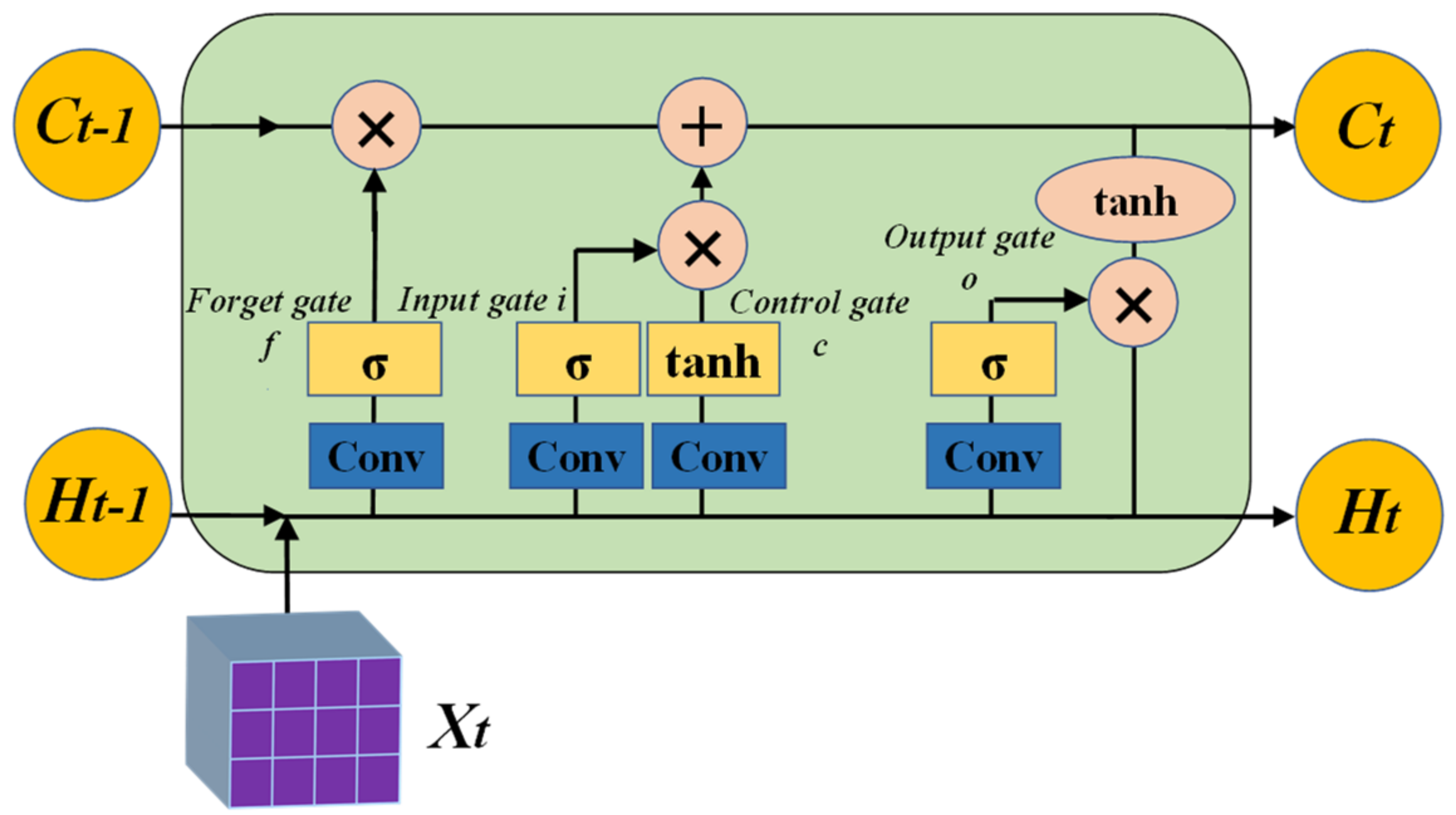
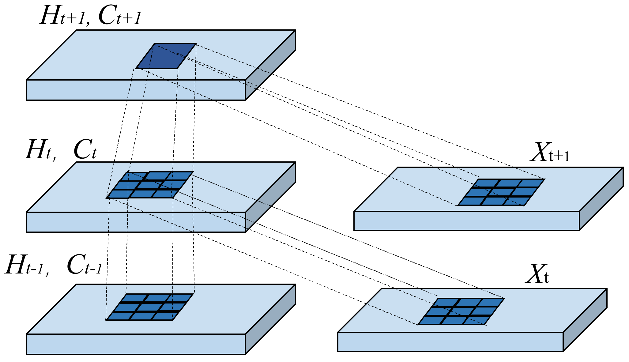
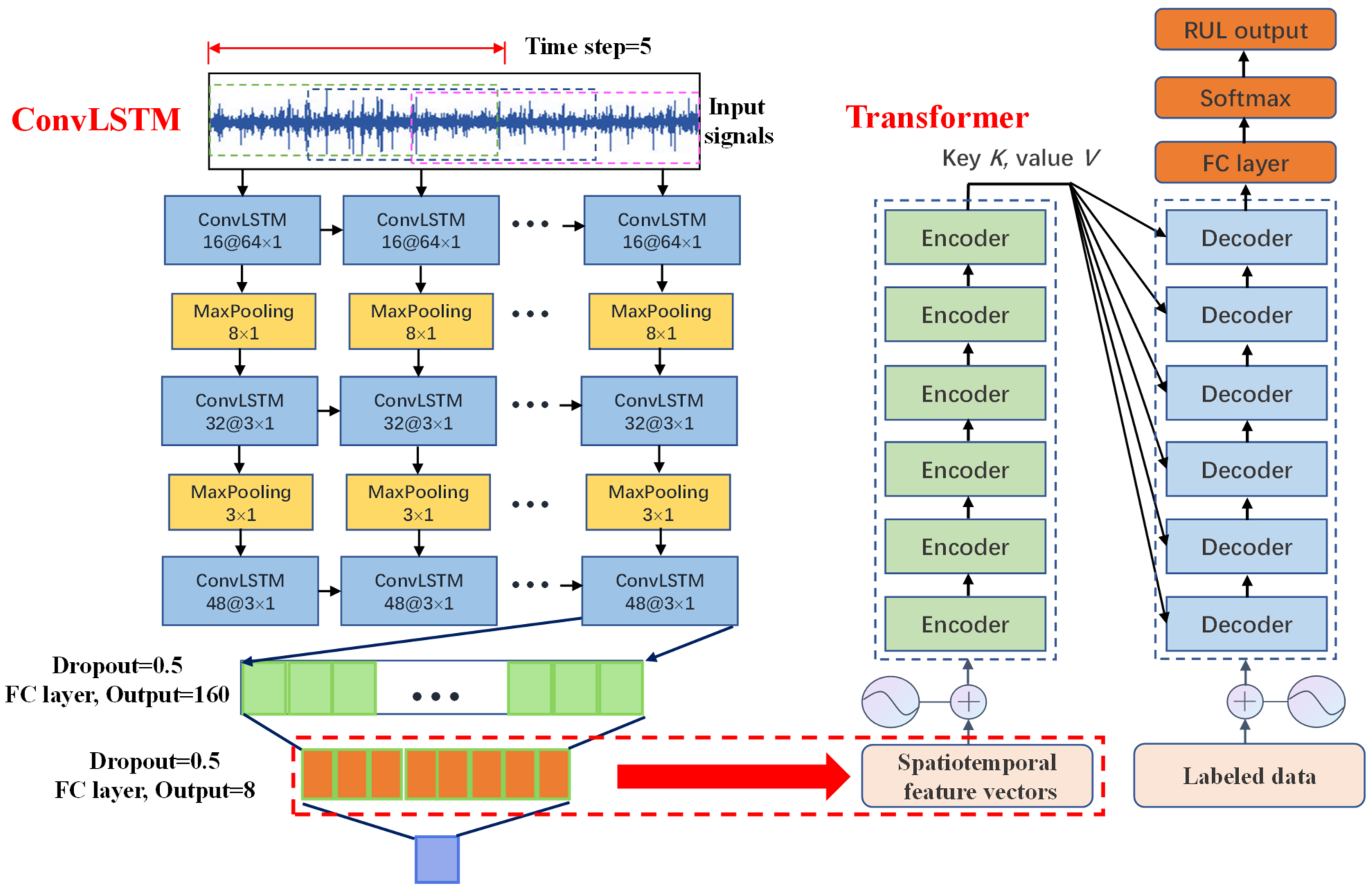
The ConvLSTM network is not a simple serial combination of CNN and LSTM. It can achieve a deep integration of CNN and LSTM by the embedded convolutional operation in the state transitions of LSTM and hence can capture spatiotemporal correlation features from the long-time degradation signal of mechanical equipment.
(2)
The ConvLSTM can directly extract the feature information reflecting the equipment degradation from the raw data without any complex signal processing techniques and prior knowledge. The transformation of high-dimensional raw data to low-dimensional features is realized through the stacking of the deep ConvLSTM network. It effectively reduces the data dimension of the raw data and ensures the efficient operation of the Transformer.
(3)
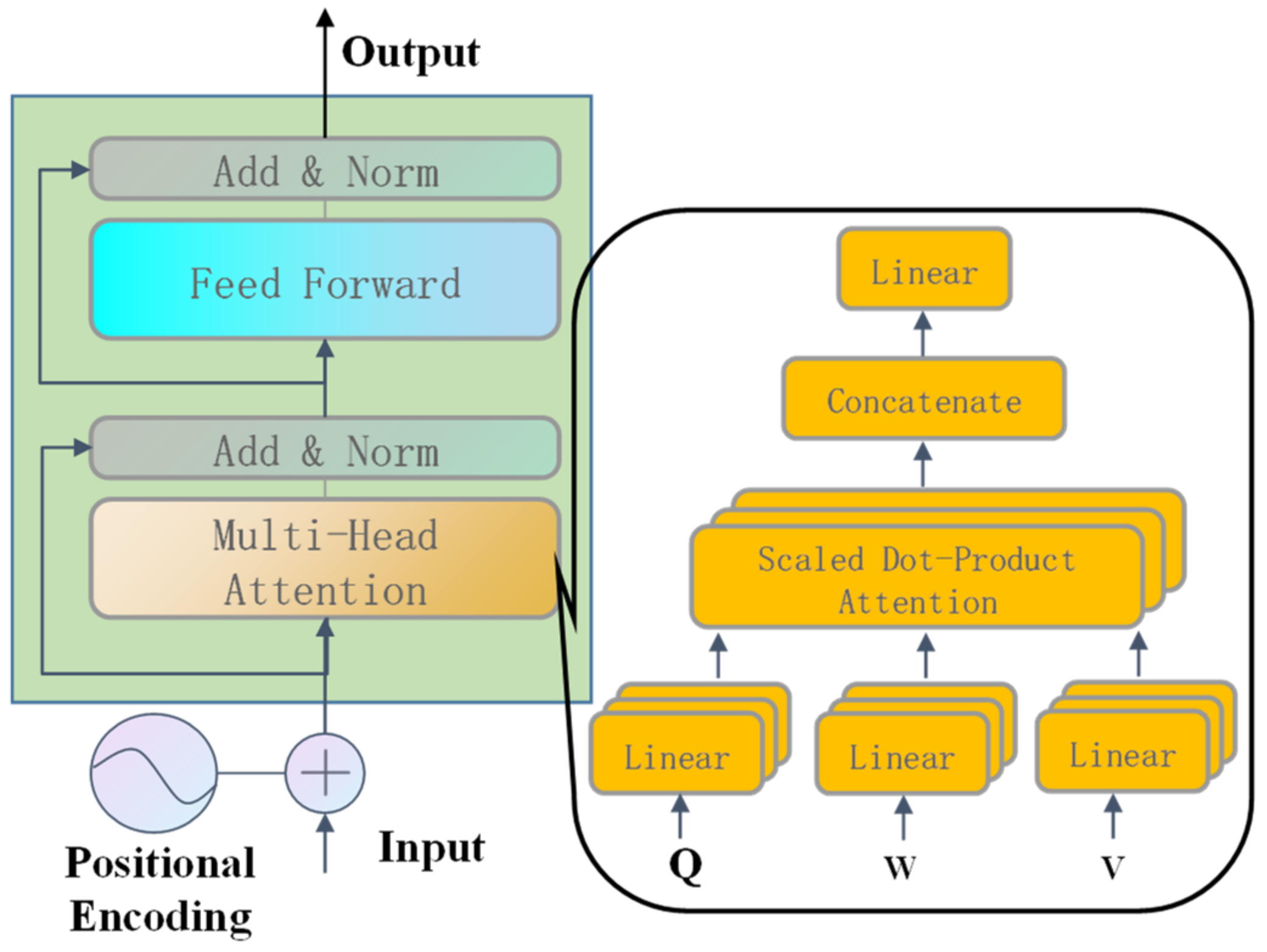
The Transformer network is constructed to perform RUL prediction analysis on the extracted spatiotemporal features and deeply explores the mapping law between deep-level nonlinear feature information and equipment service performance degradation. It further improves the accuracy of RUL prediction results and successfully expands the application of the Transformer in mechanical equipment RUL prediction.
The rest of the paper is structured as follows. The CNN, LSTM, and ConvLSTM networks are briefly described in Section 2. The Transformer framework is described in Section 3. The details of the proposed ConvLSTM-Transformer RUL prediction model are presented in Section 4. Experimental validation results and comparison analyses are illustrated in Section 5. Finally, conclusions are composed in Section 6.

2. Preliminaries

2.1. Convolutional Neural Network

CNN employs a feed-forward neural network framework, which mainly consists of convolutional layers, pooling layers, and fully connected (FC) layers. In addition, the batch normalization (BN) layer and the activation layer are also essential components of the current CNN. The convolutional layer can extract complex detailed features to the next layer by conducting convolution operations and activation operations on the features of the previous layer, which is the key component of CNN. A convolutional layer is composed of many feature maps which are convolved with one or more convolutional kernels. The convolution between the input feature map and the convolution kernel can be represented as
x l = σ ( M j x l 1 × k l + b l )
where x l is the output feature map in the lth convolutional layer, x l 1 is the input feature map, k l is the convolution kernel, b l is the bias term, M j is a collection of all output feature maps, and σ ( ) is the activation function, and the most commonly used are sigmoid, tanh, and rectified linear unit (ReLU).

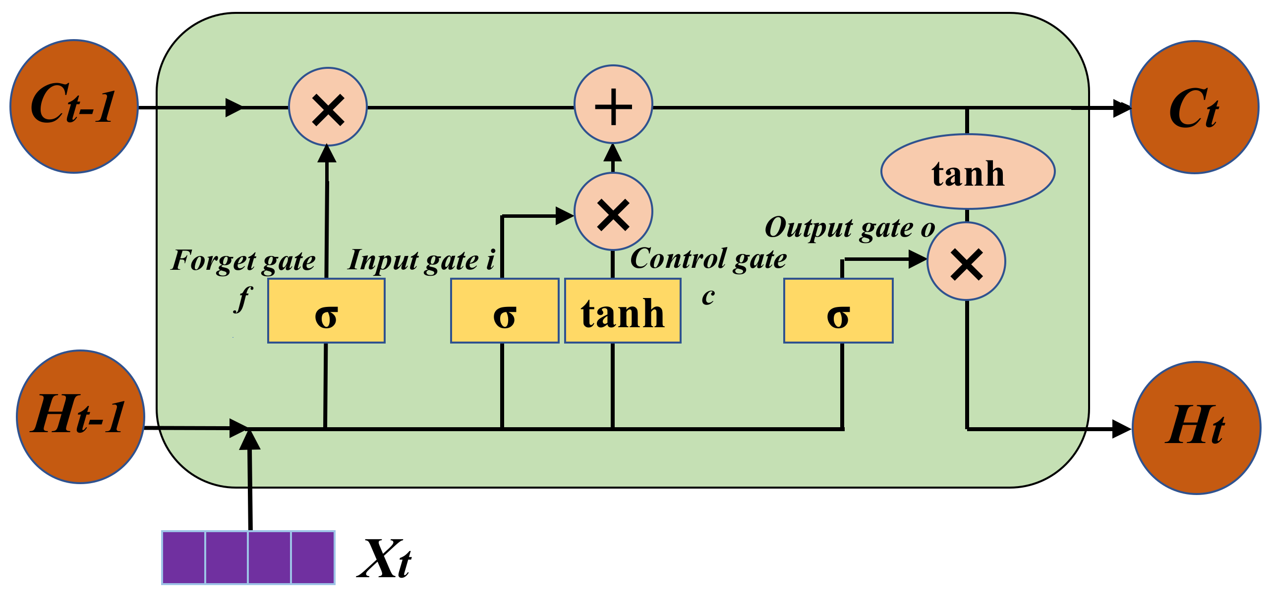
2.2. Long Short-Term Memory Network

LSTM is a variant version of RNN that is suitable for time series analysis, and it adopts a gating mechanism to effectively tackle the vanishing and exploding gradient issues in the training process. There are four gates named forget gate f, input gate i, control gate c, and output gate o in the memory cell of the LSTM. The basic structure of the LSTM cell is given in Figure 1, and it is composed of the output of previous memory cell C t 1 , the input signal at each time step X t , the output of current memory cell C t , the output of previous hidden unit H t 1 , and the output of current hidden unit H t . The forget gate decides how the contribution of the previous moment should be obtained, which will generate a value in the range of 0-1 for each data point in the C t 1 . The input gate controls how much input from the current moment will be kept in the memory cell. The control gate is used to manage the update process of the memory cell contents from C t 1 to C t by accounting for the output of f and i. The output gate determines how much the internal state at the current moment affects the external state. The symbol ⊗ indicates the multiplication of vector elements, ⊕ indicates the sum of vectors, and σ indicates the operation of activation function. The mathematical expression of the update process for the LSTM’s four gates are given as follows:
f t = σ ( W x f x t + W h f h t 1 + b f ) i t = σ ( W x i x t + W h i h t 1 + b i ) o t = σ ( W x o x t + W h o h t 1 + b o ) c t = f t × c t 1 + i t × tanh ( W x c x t + W h c h t 1 + b c ) h t = o t × tanh ( c t )
where W x f , W x i , W x o , W x c , W h f , W h i , W h o , W h c are the corresponding weight matrices, b f , b i , b o , b c are the corresponding bias vectors, and all of them will be updated in each update process.

2.3. ConvLSTM Network

The LSTM handles spatiotemporal data using full connections in the input-to-state and state-to-state transitions, whereby none of the spatial information is encoded. Therefore, although the LSTM has been demonstrated to be powerful in dealing with temporal correlation, it neglects spatial cues in the input data. The structure of the ConvLSTM cell is shown in Figure 2. It can be observed that the ConvLSTM uses 3D data as its input. In contrast, the input signal of the LSTM cell is 1D data. In addition, matrix multiplication is replaced by a convolution operation at each gate in the ConvLSTM cell, by which underlying spatial features can be captured by performing convolution operations in multi-dimensional data. In a word, the ConvLSTM cell also employs the gating mechanism but differs from the LSTM cell, it utilizes convolution operations rather than matrix multiplication to implement the input-to-state and the state-to-state transition [25], which is presented in Figure 3. Similar to the LSTM cell calculation described in Section 2.2, the mathematical expression of the ConvLSTM in the updated gates is given as follows:
f t = σ ( W x f * x t + W h f * h t 1 + W c f * c t 1 + b f ) i t = σ ( W x i * x t + W h i * h t 1 + W c i * c t 1 + b i ) o t = σ ( W x o * x t + W h o * h t 1 + W c o * c t + b o ) c t = f t × c t 1 + i t × tanh ( W x c * x t + W h c * h t 1 + b c ) h t = o t × tanh ( c t )
where ‘∗’ indicates convolution, ‘×’ indicates Hadamard product, and W c f , W c i , W c o indicate the weight matrices. All the weight matrices and bias vectors will be updated in each update process.

3. Transformer Neural Network

The RNN can process input data sequentially to acquire the cumulative representation for the model input. The predicted result is only relevant to the input sequence at the current moment and the previous moments. However, it should be noted that the RNN takes a serial processing mode that strictly relies on time order. The sequential execution process restricts the parallelization ability of the network in the training process and the inference process. Although the gate mechanism structure adopted by RNNs, such as LSTM and BiLSTM, alleviates the problem of long-range dependencies on long-time sequence signals to some extent, RNN-based models are still unable to effectively overcome the particularly long-term dependence phenomenon [30]. The Transformer network shows great advantages in the prediction task for long-time series because it adopts parallel computing, which is in line with the current computer hardware GPU environment. The multi-headed self-attention mechanism can effectively learn long-range dependencies.
The model architecture of the Transformer mainly consists of two main parts, encoder and decoder architectures, in which the recurrent layers most commonly used are replaced by the multi-headed self-attentions. The structure of an encoder is shown in Figure 4. Because the Transformer is a sequence-to-sequence network, which is entirely based on self-attention mechanisms and does not contain recurrences and convolutions, the relative or absolute position information must be injected into the input sequence to ensure that the Transformer network utilizes the order of the sequence. Sine and cosine functions which have different frequencies are used for positional encoding, and the process can be expressed as:
P E ( p o s , 2 i ) = sin ( p o s / 10,000 2 i / d x ) P E ( p o s , 2 i + 1 ) = cos ( p o s / 10,000 2 i / d x )
where pos denotes the position of the specified data point in the sequence, 2i and 2i+1 denote the channel index, and dx is the embedding dimension, generally dx = 512.
The positional encoding in each dimension corresponds to a sinusoid and the wavelength is a geometric progression from 2π to 10,000−2π. The position information is composed of sine and cosine functions of different frequencies alternating with each other. In practice, the sequence after positional encoding is obtained by summing each vector in the input sequence with the corresponding position information. It should be noted that the dimension of the input sequence increases dramatically after the positional encoding operation. Assuming that the dimensions of the input data are M × N, M is the number of data samples and N is the number of data points in the samples. The dimensions of the input data increase to M × N × dx after the positional encoding. When M = 3 and N = 4, the dimensionality increase process of positional encoding is shown in Figure 5. The degradation of mechanical equipment is a long-term process, and the collected sample signals are usually long-time sequences. That is to say, the values of M and N are often very large. As a result, the data dimension after the positional encoding increases significantly, and the number of model parameters increases dramatically, which makes the Transformer training very difficult and prone to overfitting and other problems. For this reason, this paper proposes to use the ConLSTM network to extract the low-dimensional spatiotemporal feature vectors from the long-time degradation sequence, which effectively reduces the amount of data fed into the Transformer network.
The first layer of the encoder is the multi-head attention composed of some attention layers in parallel, which uses the attention “Scaled Dot-Product Attention” to implement the mapping of the query matrix Q to the key matrix K and the value matrix V to obtain the weighted sum of the values V:
A ttention ( Q , K , V ) = S oft max ( Q K d ) V
Q = X t W Q K = X t W K V = X t W V
where W Q , W K , W V are the weight matrixes corresponding to Q, K, and V and d is the dimension. First, the dot products of the query Q and all keys K are calculated, then each are divided by d and the softmax function is applied to acquire the weights on values. The multi-head attention mechanism obtains the values in different subspaces by concatenating several single attentions and finally obtains the attention information in all subspaces after the parallel operation. The residual connection is employed around each of the two sub-layers to extend the depth of the network and eliminate the vanishing gradient problem.
The structure of a decoder is presented in Figure 6. Different from the encoder, the first layer of the decoder is the masked multi-head attention, which is implemented by the masking operation. The purpose of the masking operation is to make the decoder only focus on the input sequence at the current moment and the previous moments. The realization process of the masking operation is to generate an upper triangular matrix and set the values of the upper triangle to zero and apply this matrix to cover each sequence and achieve the purpose of concealing the future information. It works by adding to the multi-head attention to prevent each position from appearing in future positions, which effectively avoids the auto-regressive property. The process of the masking operation is given in Figure 7. The input data of the decoder are y 1 , y 2 , y 3 y T , and the result after positional encoding is α 1 , α 2 , α 3 α T in the figure. The shaded part of the matrix processed by the multi-head self-attention layer is the upper triangular matrix, and the covered values are all set to zero. After that, the flowed information is processed by lay normalization as the query Q and the output of the previous encoder as the key K and value V, which are fed together into the next multi-head attention layer and finally output by a fully connected feed-forward network.

4. Convlstm-Transformer Model

The proposed ConvLSTM-Transformer model can fully integrate the advantages of the CNN, LSTM, and Transformer networks. The ConvLSTM network is used to extract spatiotemporal features from the long-time degradation signals and reduce the data dimensionality of the input to the Transformer network. The Transformer is applied to perform RUL prediction on the extracted multidimensional features. In actual engineering, we cannot continuously monitor the whole operating life of the equipment but only sample at intervals, which results in collecting a small amount of data for a single sampling signal only related to the current degradation state of the equipment. To address this issue, a time step embedding strategy is used to process the collected raw signal samples after normalization. The single-channel 2D matrix can be given as:
X k = [ x k ; x k + 1 ; ; x k + t 1 ]
where k is the serial number of the raw 1D bearing signal sample and t is the time step. The time step of the proposed method is set to t = 5 according to the literature [14]. The 3D input data that is fed into the ConvLSTM network is composed of multiple single-channel matrices. The 3D input data of the proposed method is shown in Figure 8. The number of the 3D data channel is set to n − 4, and n denotes the number of the raw 1D bearing signals.
The architecture of the proposed ConvLSTM-Transformer model is shown in Figure 9. The ConvLSTM network consists of three ConvLSTM layers, two max pooling layers, and three FC layers. The first ConvLSTM layer with a convolutional kernel size of 64 × 1 is designed to extract spatiotemporal features of the input signals using a larger receptive field, followed by two ConvLSTM layers with a small convolutional kernel size of 3 × 1 to extract more detailed spatiotemporal feature information. The first two ConvLSTM layers are followed by a max pooling layer, which can further compress the data dimension and reduce the number of network parameters. At the end of the network are three FC layers, in which the second FC layer contains eight neurons and its output is considered to be the spatiotemporal feature vectors that are fed into the Transformer network. In addition, the Dropout layer is added to the FC layers to enhance the robustness of the network and avoid overfitting. The parameters of the ConvLSTM network are upgraded by minimizing the training error, and the optimization process of the network model employs the Adam algorithm. The Transformer network is composed of six sequentially stacked encoder blocks and six decoder blocks. The spatiotemporal feature vectors obtained by the ConvLSTM network are fed into the encoder block, and the ratio of the actual RUL values of each sample signal to their respective whole lifetime is fed into the decoder block as the labeled data. In practice, it is necessary to normalize the labeled data to be in the range of [0, 1] to eliminate the influence of different bearings with very wide ranges of a lifetime. The end of the Transformer network is an FC layer that outputs the RUL prediction result using the softmax function. The training process of the Transformer network is equivalent to solving a supervised multi-classification problem. The Mean Square Error (MSE) is calculated as a loss function of the Transformer during training, and the Adam algorithm is chosen to minimize the training error by iteratively updating the network parameters.

5. Experimental Verification

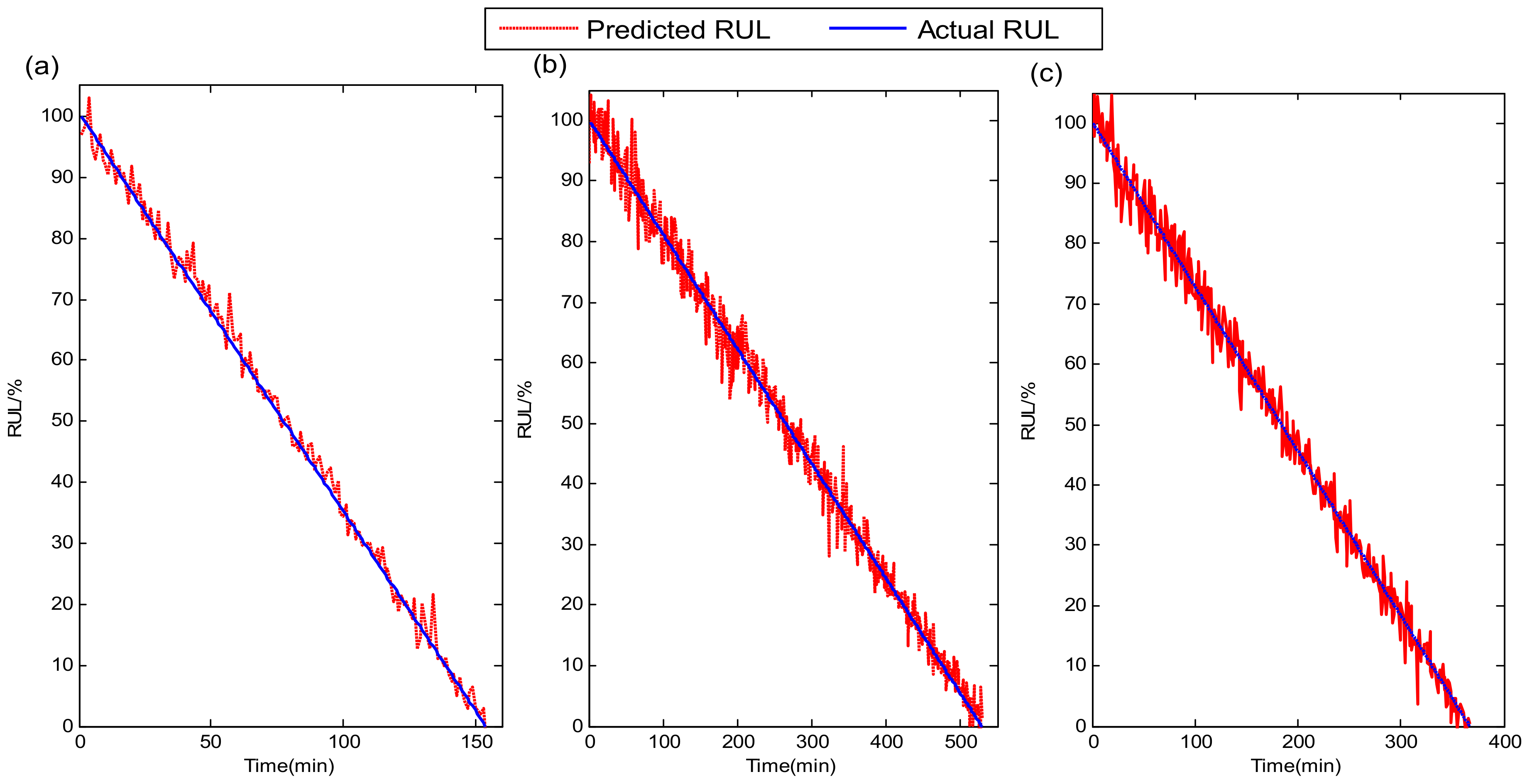
5.1. PHM 2012 Bearing RUL Prediction

To validate the effectiveness of the proposed ConvLSTM-Transformer model in this paper, the experimental verification is first carried out on the PHM 2012 Challenge dataset. The PRONOSTIA accelerated aging test platform was used to simulate the process of the bearing lifetime degradation, which is shown in Figure 10. The run-to-failure vibration signals for the bearing’s whole life were collected on the platform. With an acquisition time of 0.1 s, the signal was sampled at 25.6 kHz and recorded every 10 s. In the accelerated aging test, there are three operating conditions for 17 tested bearings, and detailed experimental information can be found in the literature [31]. The selection of the training set and testing set in this paper is given in Table 1. Because these tested bearings are subjected to horizontal loading during the testing, horizontal vibration measurements provide more helpful information in tracking bearing degradation than vertical vibration signals; therefore, horizontal signals are used for analysis.
The whole-life vibration signals of bearing1_3, bearing2_5, and bearing3_2 in the PHM 2012 dataset are presented in Figure 11, respectively. As a whole, the waveform amplitudes of the vibration signals are relatively small in the early testing phase, while the waveform amplitudes increase sharply in the late fault phase when serious faults occur. However, due to the complexity and high randomness of each bearing’s whole-life signal change process under different operating situations, as well as the various types of damage failure that eventually emerge, it undoubtedly increases the difficulty of the RUL prediction for the testing bearings.
The ConvLSTM network is constructed to obtain the spatiotemporal feature vectors from the long-time degradation signals of the bearings, and then they are fed into the Transformer network. Following the training of the model, the RUL prediction is performed for each testing bearing, and the results are shown in Figure 12. The red dashed line in this figure indicates the RUL prediction results of the proposed method, and the blue solid line indicates the real RUL results of different testing bearings. It can be observed that the RUL prediction results of these four tested bearings are mostly agreeable with the real RUL results, and the trend and monotonicity changes are also identical, which confirms the effectiveness of the proposed method.

5.2. XJTU-SY Bearing RUL Prediction

The public XJTU-SY whole-life bearing dataset is also selected for experimental analysis to further confirm the effectiveness of the proposed method in this section. In the experiments, the sampling frequency is set to 25.6 kHz, the sampling duration time is 1.28 s, and the sampling interval time is 1min. The XJTU-SY bearing lifetime dataset contains a total of 15 whole-life vibration signals of LDK UER204 rolling element bearings under three operation conditions, and detailed information about this experiment can be found in the literature [32]. The selection of the training set and testing set is presented in Table 2.
The temporal waveforms of whole-life vibration signals for the three tested bearings under different operation conditions are given in Figure 13. It can be seen from the figure that even for the same type of bearings, their life ranges and waveform amplitude variations are very different under three operating conditions. RUL results of the above three tested bearings using the proposed method are shown in Figure 14. Although the number of signal samples collected for each tested bearing in the XJTU-SY bearing dataset is smaller than in the PHM 2012 bearing dataset, it can be observed that the proposed method still gives accurate RUL prediction results for the tested bearings. It further confirms that the proposed method could achieve high performance for different bearings under various operating conditions.
The computational cost is an important influencing factor for the application of the RUL prediction module in real industrial applications. All the experiments are tested on a computer with an Intel Core i7-9700K CPU (Intel, Santa Clara, CA, USA) and NVIDIA RTX 2070 SUPER GPU (Nvidia Corporation, Santa Clara, CA, USA). The computational cost of the proposed approach mainly consists of two parts, which are the computational costs of the ConvLSTM and the Transformer. The computational cost results of the proposed approach for part of the experiments are given in Table 3. The operation of the ConvLSTM module is more computationally expensive than the Transformation module. On the one hand, to achieve the purpose of spatiotemporal feature extraction and data reduction, the ConvLSTM is used to deal with the raw bearing whole-life signals. Therefore, the input data of the ConvLSTM is considerably larger than the Transformer. On the other hand, the Transformer has a high operation efficiency because it allows for more parallelization. Moreover, the computation cost of test data from the PHM 2012 dataset is more expensive than the XJTU-SY dataset. A possible explanation is that the XJTU-SY dataset has a small amount of data. The number of collected bearing signal samples in the XJTU-SY dataset is less than in the PHM 2012 dataset. On the whole, the execution time of the proposed approach is acceptable.

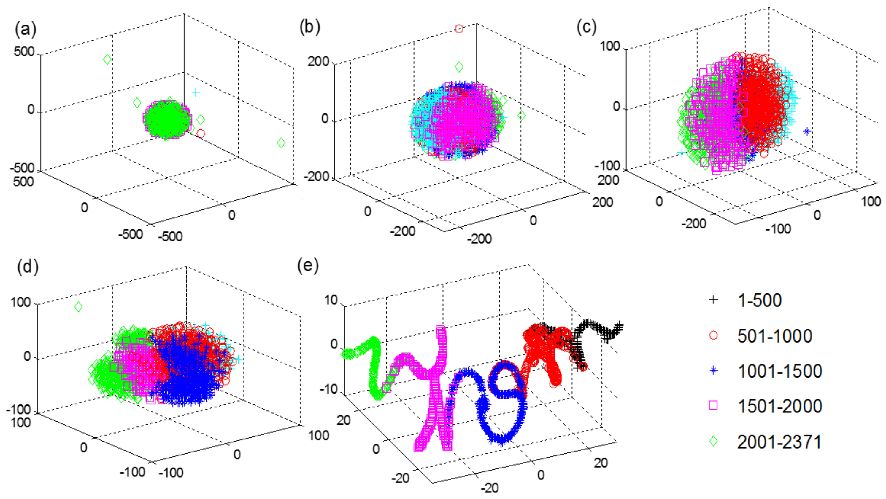
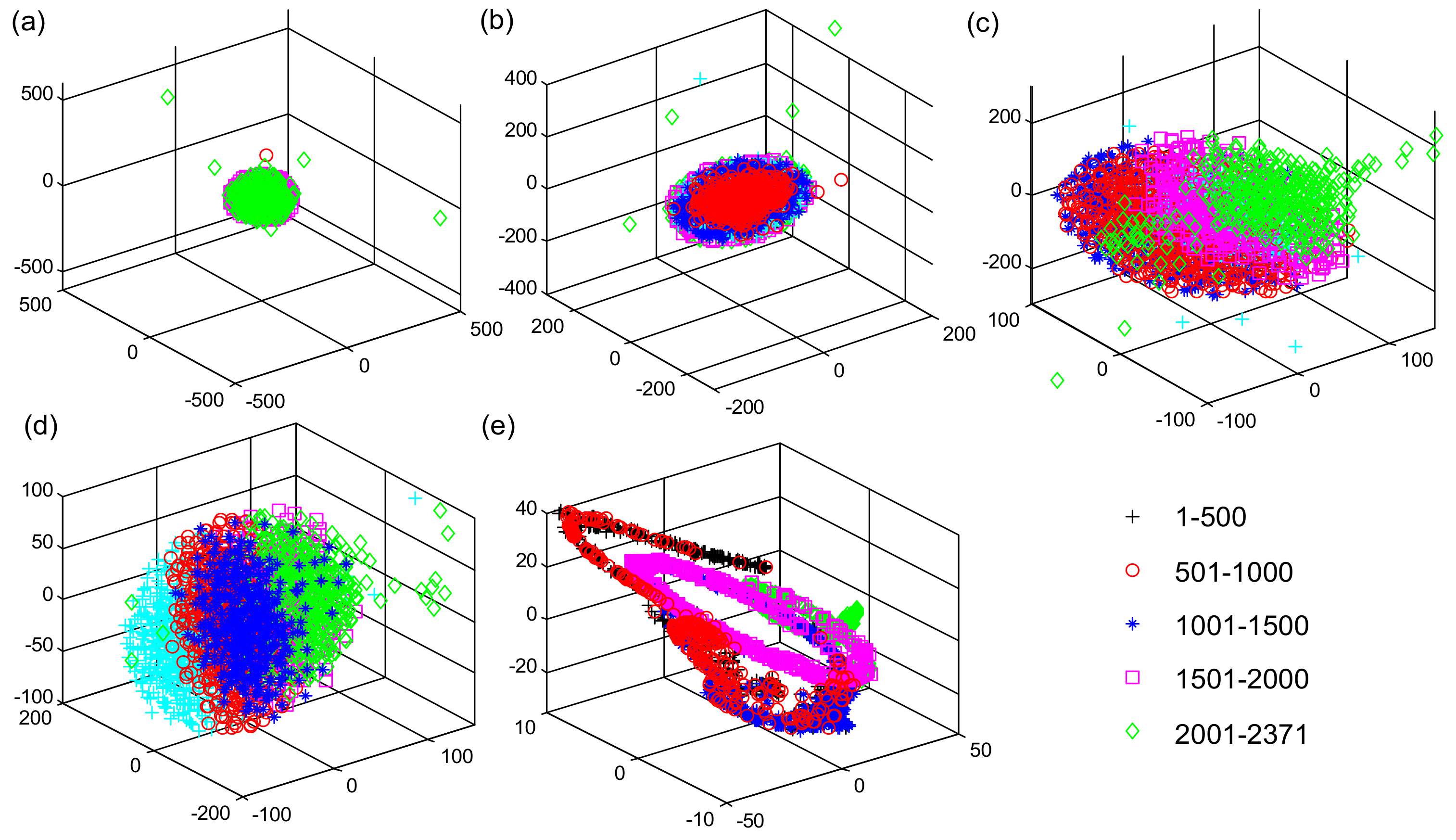
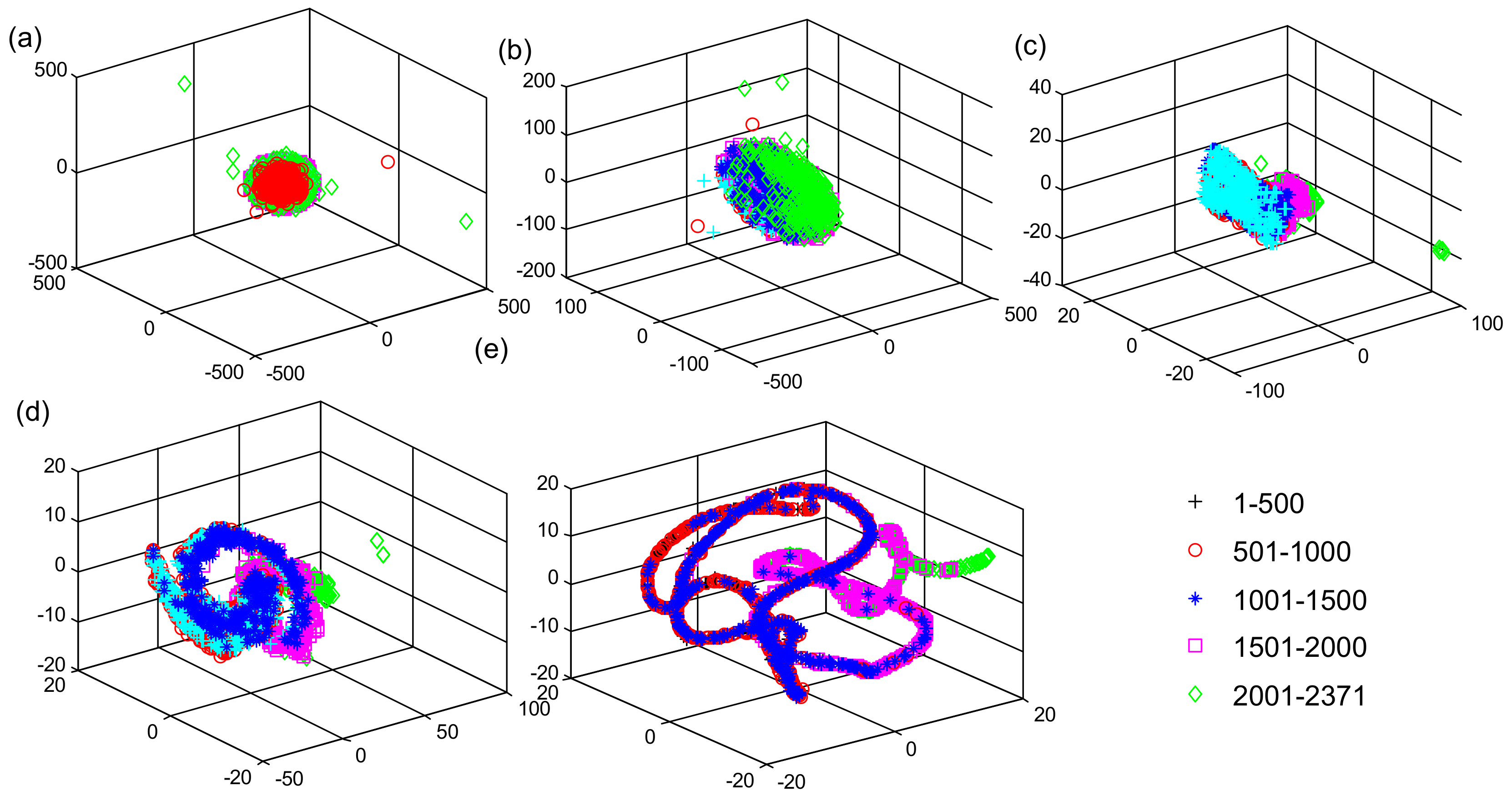
5.3. Spatiotemporal Feature Visualization Analysis

To better investigate the distribution characteristics of the spatiotemporal features extracted by the proposed ConvLSTM network for the long-time degradation signals, a nonlinear dimensionality reduction method named t-distributed stochastic neighbor embedding (t-SNE) algorithm [33] is used to generate three-dimensional (3D) representations of high-dimensional feature maps at different hidden layers of the ConvLSTM network. The signal samples of Bearing1_3 in the PHM 2012 dataset are selected for visualization analysis. There are 2731 signal samples in the whole-life period of Bearing1_3 after the operation of five time-step embeddings, and all the signal samples are divided into five groups according to chronological order. The visualization results of the high-dimensional features at the network input, ConvLSTM1 layer, ConvLSTM2 layer, ConvLSTM3 layer, and the second FC (FC2) layer of the proposed ConvLSTM network are shown in Figure 15. The dots with different colors and different types in the figure represent five different clusters of all the signal samples. At the input of the ConvLSTM network, all the feature dots are completely gathered together and cannot be identified. With the increase in the network layers, these feature dots corresponding to different sampling times start to be separated gradually until the last FC2 layer. Although there are still slight pieces of overlap, the majority of dots are clearly separated and clustered together in chronological order, which confirms that the proposed ConvLSTM network is capable of learning the spatiotemporal correlation features from the long-time degradation sequences of bearing.
The CNN and LSTM with the same network framework are used for 3D representations of high-dimensional feature visualization analysis. The visualization results of the same data at the same stages of the CNN and LSTM networks are shown in Figure 16 and Figure 17, respectively. It can be observed that as the layers of the CNN and LSTM networks increase, the feature dots corresponding to different sampling times start to be gradually separated and clustered. However, these feature dots are heavily overlapped even until the output of the last FC2 layers of the CNN and LSTM networks. By visualization comparative analysis, due to some inherent shortcomings of the CNN and LSTM networks, it is difficult to categorize the features extracted from the long-time degradation sequences in chronological order, which cannot accurately reflect the feature evolution process during the whole-life cycle of bearings.

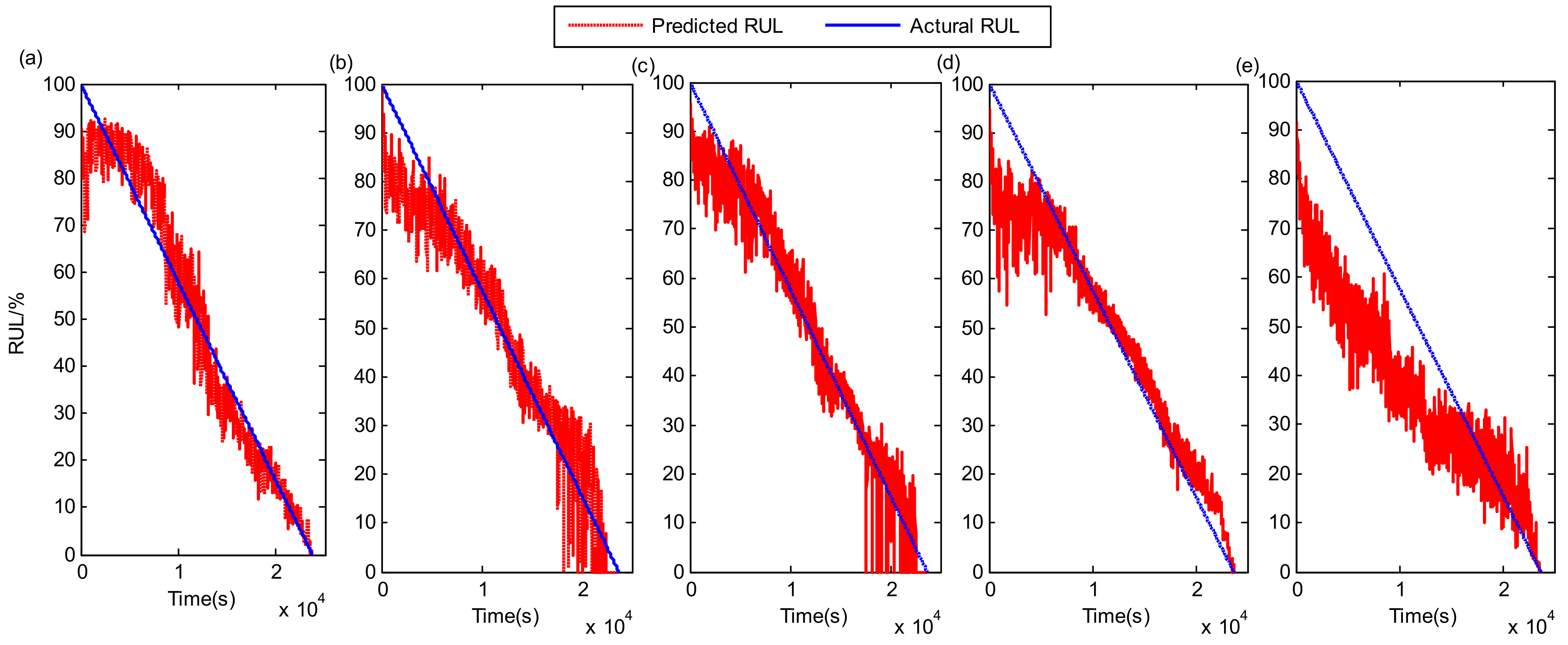
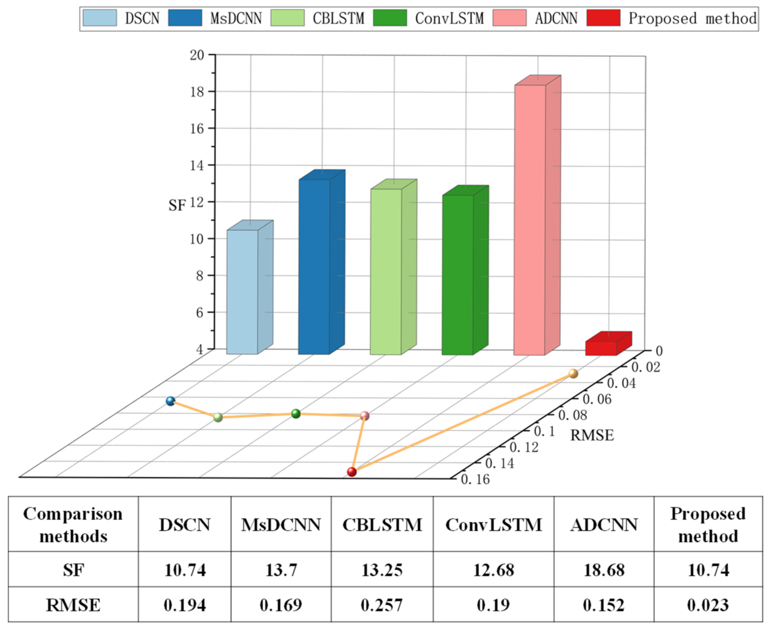
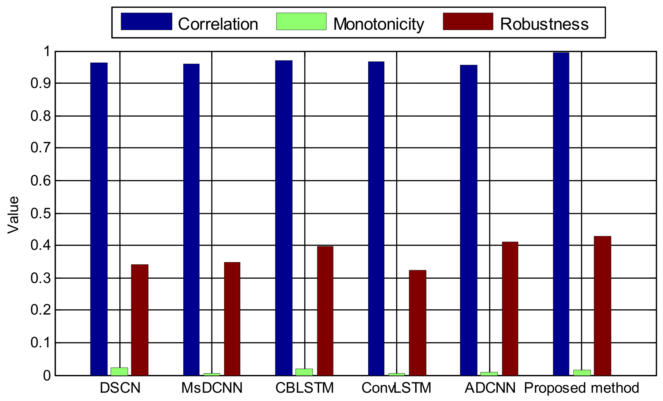
5.4. Comparison with the State-of-the-Art methods

In this section, five state-of-the-art network modules are used to predict the bearing RUL for exhibiting the superiority of the proposed method, including deep separable convolutional network (DSCN) [14], multi-scale deep convolutional neural network (MsDCNN) [34], convolutional bi-directional long short-term memory network (CBLSTM) [35], the proposed ConvLSTM network, and attentive dense convolutional neural network (ADCNN) [36]. The RUL prediction results of the above comparison methods for the tested bearing1_3 in the PHM 2012 dataset are given in Figure 18. Compared with the RUL result of the proposed method in Figure 10, although the overall tendencies of the RUL estimations for all the methods are consistent, it can be observed that the predicted result of the proposed method is most similar to the actual RUL result. Two commonly used evaluation metrics in the field of RUL prognostics, the scoring function (SF) and root mean square error (RMSE) [13,14,34,35], are employed to quantitatively assess the accuracy of the RUL prognostic result for the above methods. The RUL prediction result is more accurate with a lower SF value and RMSE value. The literature [14] provided a full explanation of how the two metrics were calculated. It should be noted that each test was repeated five times to improve the reliability of the RUL prediction results, and all the metric values appearing in this paper are the average of the five test results. The SF and RMSE results of the above five methods are shown in Figure 19. It can be clearly observed that the proposed method in this paper has the smallest RMSE and SF values compared to the four comparison methods, and the gaps of SF values and RMSE values with the four comparison methods are very significant, which confirms that the proposed ConvLSTM-Transformer method has higher accuracy in bearing RUL estimation.
To further comprehensively evaluate the RUL prediction performance of the above five prognostic models, three evaluating functions, correlation, monotonicity, and robustness, are chosen to study the RUL prediction results of different methods. Correlation describes how the prediction result varies with time, monotonicity reflects the increasing or decreasing trend of the prediction result, and robustness represents the variability of the prediction result with random fluctuations. The larger the three evaluating functions, the better the comprehensive performance of the prognostic model. These three evaluating functions can be computed as follows, and detailed information about them can be found in the literature [37].
C o r r ( F , T ) = K k f T ( k ) t k k f T ( k ) t k k t k K k f T ( k ) 2 ( k f T ( k ) ) 2 K k ( t k ) 2 ( k t k ) 2
M on ( F ) = 1 K 1 k δ ( f T ( k + 1 ) f T ( k ) ) k δ ( f T ( k ) f T ( k + 1 ) )
R o b ( F ) = 1 K k exp ( f R ( k ) f ( k ) )
The results of these three evaluating functions for PHM 2012 beaing1_3 RUL prediction result are shown in Figure 20. The correlation value and robustness value of the proposed method are larger than those of the five comparison methods, and the monotonicity values of the five methods are small and close to each other. Based on this analysis, it can be concluded that the proposed approach has outstanding comprehensive RUL prediction performance.

5.5. Generalization Capability Analysis

The generalization capability of the proposed model is analyzed in this section. There are mainly two groups of working conditions for model training and testing when the experimental data are from the PHM 2012 dataset. The number of training bearing signal samples in the first group is six, and that in the second group is eight. They are easily obtained from Table 1. A preliminary conclusion can be drawn that when the number of training signal samples from different working conditions is reduced from eight to six, the proposed model test results still have good accuracy. Next, the generalization capability of the proposed model is further verified by reducing the number of training signal samples in the first group, in which the Bearing1_3 signal is the test signal sample. The number of training signal samples is set to five in the first group, including Bearing1_1, Bearing1_2, Bearing1_4, Bearing1_5, and Bearing1_6. Then, the number of training signal samples is set to four, including Bearing1_1, Bearing1_2, Bearing1_4, and Bearing1_5. Finally, the number of training signal samples is set to three, including Bearing1_1, Bearing1_2, and Bearing1_4. The SF and RMSE of the RUL prediction results for the above discussions are given in Table 4. As can be seen from Table 4, the RUL prediction accuracy of the proposed model is only slightly decreased when the number of training data samples was reduced from six to four. The difference between them is not significant, which indicates that the generalization capability of the proposed model is acceptable.

6. Conclusions

At present, convolution neural network (CNN) and long short-term memory (LSTM) are the most commonly used deep neural networks, but they suffer from some inherent drawbacks in their application to RUL prediction. CNN is not appropriate for analyzing temporal signals and cannot learn time-sequence features. The LSTM is based on serial processing mode and cannot extract spatial correlations from a long-time degradation sequence. Aiming at the above problems, a novel combination network model of ConvLSTM and Transformer, which is based on the idea of “Extracting spatiotemporal features and applying them to RUL prediction”, is proposed for mechanical equipment RUL prediction in this paper. Rather than simply serially connecting a CNN to an LSTM, the ConvLSTM network performs convolutional operations on both input-to-state and state-to-state transitions of the LSTM. It incorporates the advantages of CNN and LSTM and can directly extract spatiotemporal features from long-time degradation sequences. The Transformer based entirely on attention mechanisms can acquire the dependency information between arbitrary vectors in long-time sequences and deeply explore the mapping law between deep-level nonlinear feature information and equipment service performance degradation. The low-dimensional spatiotemporal feature vectors extracted by the ConvLSTM network are fed into the Transformer network to guarantee efficient operation and yield RUL prediction results.
The proposed ConvLSTM-Transformer is experimentally validated by using the PHM 2012 Challenge dataset and the XJTU-SY whole-life bearing dataset. The scoring function (SF) and root mean square error (RMSE) show that the proposed approach has a higher accuracy of RUL prediction results through the comparative analysis. Furthermore, comparative calculations of three evaluating functions of correlation, monotonicity, and robustness demonstrate that the proposed approach has excellent comprehensive RUL prediction performance. Although the ConvLSTM-Transformer model has achieved good RUL prediction results, there are still some drawbacks that needed to be improved in the future, such as simplifying the proposed network structure and improving the optimization efficiency of the network training process.

Author Contributions

Methodology F.D.; conceptualization, Z.C.; software, Y.L.; validation, S.Y.; investigation, R.H.; resources, L.L.; writing—original draft preparation, F.D.; writing—review and editing, F.D. All authors have read and agreed to the published version of the manuscript.

Funding

This research was funded by Deng F. of funder, grant number 12272243, A202101017. This research was funded by Yang S. of funder, grant number 12032017, 11790282, 2020YFB2007700. This research was funded by Liu Y. of funder, grant number 20310803D, A2020210028. This research was funded by Hao R. of funder, grant number 11872256. This research was funded by Lyu L. of funder, grant number E2021210011.

Institutional Review Board Statement

Not applicable.

Informed Consent Statement

Not applicable.

Data Availability Statement

Conflicts of Interest

The authors declare no conflict of interest.

References

  1. Lei, Y.; Li, N.; Gontarz, S.; Lin, J.; Radkowski, S.; Dybala, J. A Model-Based Method for Remaining Useful Life Prediction of Machinery. IEEE Trans. Reliab. 2016, 65, 1314–1326. [Google Scholar] [CrossRef]
  2. Lei, Y.; Li, N.; Guo, L.; Li, N.; Yan, T.; Lin, J. Machinery health prognostics: A systematic review from data acquisition to RUL prediction. Mech. Syst. Signal Process. 2018, 104, 799–834. [Google Scholar] [CrossRef]
  3. Peng, W.; Ye, Z.-S.; Chen, N. Joint online RUL prediction for multi-deteriorating systems. IEEE Trans. Ind. Informat. 2019, 15, 2870–2878. [Google Scholar] [CrossRef]
  4. Zhao, R.; Yan, R.; Chen, Z.; Mao, K.; Wang, P.; Gao, R.X. Deep learning and its applications to machine health monitoring. Mech. Syst. Signal Process. 2019, 115, 213–237. [Google Scholar] [CrossRef]
  5. Benkedjouh, T.; Medjaher, K.; Zerhouni, N.; Rechak, S. Remaining useful life estimation based on nonlinear feature reduction and support vector regression. Eng. Appl. Artif. Intell. 2013, 26, 1751–1760. [Google Scholar] [CrossRef]
  6. Gebraeel, N.; Lawley, M.; Liu, R.; Parmeshwaran, V. Residual life predictions from vibration-based degradation signals: A neural network approach. IEEE Trans. Ind. Electron. 2004, 51, 694–700. [Google Scholar] [CrossRef]
  7. Moosavian, A.; Ahmadi, H.; Tabatabaeefar, A.; Sakhaei, B. An appropriate procedure for detection of journal-bearing fault using power spectral density, k-nearest neighbor and support vector machine. Int. J. Smart Sens. Intell. Syst. 2017, 5, 685–700. [Google Scholar] [CrossRef] [Green Version]
  8. Dong, M.; He, D. A segmental hidden semi-Markov model (HSMM)-based diagnosticsand prognostics framework and methodology. Mech. Syst. Signal Process. 2007, 21, 2248–2266. [Google Scholar] [CrossRef]
  9. Chen, H.; Wang, J.; Tang, B.; Xiao, K.; Li, J. An integrated approach to planetary gearbox fault diagnosis using deep belief networks. Meas. Sci. Technol. 2016, 28, 025010. [Google Scholar] [CrossRef]
  10. Lei, Y.; Jia, F.; Lin, J.; Xing, S.; Ding, S.X. An Intelligent Fault Diagnosis Method Using Unsupervised Feature Learning Towards Mechanical Big Data. IEEE Trans. Ind. Electron. 2016, 63, 3137–3147. [Google Scholar] [CrossRef]
  11. Ren, L.; Sun, Y.; Wang, H.; Zhang, L. Prediction of Bearing Remaining Useful Life with Deep Convolution Neural Network. IEEE Access 2018, 6, 13041–13049. [Google Scholar] [CrossRef]
  12. Zhu, J.; Chen, N.; Peng, W. Estimation of Bearing Remaining Useful Life Based on Multiscale Convolutional Neural Network. IEEE Trans. Ind. Electron. 2018, 66, 3208–3216. [Google Scholar] [CrossRef]
  13. Deng, F.; Bi, Y.; Liu, Y.; Yang, S. Deep-Learning-Based Remaining Useful Life Prediction Based on a Multi-Scale Dilated Convolution Network. Mathematics 2021, 9, 3035. [Google Scholar] [CrossRef]
  14. Wang, B.; Lei, Y.; Li, N.; Yan, T. Deep separable convolutional network for remaining useful life prediction of machinery. Mech. Syst. Signal Process. 2019, 134, 106330. [Google Scholar] [CrossRef]
  15. Zhao, R.; Wang, D.Z.; Yan, R.Q.; Mao, K.Z.; Shen, F.; Wang, J.J. Machine Health Monitoring Using Local Feature-Based Gated Recurrent Unit Networks. IEEE Trans. Ind. Electron. 2017, 65, 1539–1548. [Google Scholar] [CrossRef]
  16. Liu, J.; Li, Q.; Chen, W.; Yan, Y.; Qiu, Y.; Cao, T. Remaining useful life prediction of PEMFC based on long short-term memory recurrent neural networks. Int. J. Hydrog. Energy 2019, 44, 5470–5480. [Google Scholar] [CrossRef]
  17. Li, X.; Zhang, L.; Wang, Z.; Dong, P. Remaining useful life prediction for lithium-ion batteries based on a hybrid model combining the long short-term memory and Elman neural networks. J. Energy Storage 2019, 21, 510–518. [Google Scholar] [CrossRef]
  18. Shen, Z.; Fan, X.; Zhang, L.; Yu, H. Wind speed prediction of unmanned sailboat based on CNN and LSTM hybrid neural network. Ocean Eng. 2022, 254, 111352. [Google Scholar] [CrossRef]
  19. Agga, A.; Abbou, A.; Labbadi, M.; El Houm, Y.; Ali, I.H.O. CNN-LSTM: An efficient hybrid deep learning architecture for predicting short-term photovoltaic power production. Electr. Power Syst. Res. 2022, 208, 107908. [Google Scholar] [CrossRef]
  20. Chu, C.-H.; Lee, C.-J.; Yeh, H.-Y. Developing Deep Survival Model for Remaining Useful Life Estimation Based on Convolutional and Long Short-Term Memory Neural Networks. Wirel. Commun. Mob. Comput. 2020, 2020, 8814658. [Google Scholar] [CrossRef]
  21. Vaswani, A.; Shazeer, N.; Parmar, N.; Uszkoreit, J.; Jones, L.; Gomez, A.N.; Kaiser, L.; Polosukhin, I. Attention is all you need. arXiv 2017, arXiv:1706.03762. [Google Scholar]
  22. Plizzari, C.; Cannici, M.; Matteucci, M. Spatial temporal transformer network for skeleton-based action recognition. In Proceedings of the International Conference on Pattern Recognition, Virtual Event, 10–15 January 2021; Springer: Cham, Switzerland, 2021; pp. 694–701. [Google Scholar]
  23. Dai, Z.; Yang, Z.; Yang, Y.; Carbonell, J.; Le, Q.V.; Salakhutdinov, R. Transformer-xl: Attentive language models beyond a fixed-length context. arXiv 2019, arXiv:1901.02860. [Google Scholar]
  24. Xu, M.; Dai, W.; Liu, C.; Gao, X.; Lin, W.; Qi, G.J.; Xiong, H. Spatial-temporal transformer networks for traffic flow forecasting. arXiv 2020, arXiv:2001.02908. [Google Scholar]
  25. Yu, C.; Ma, X.; Ren, J.; Zhao, H.; Yi, S. Spatio-temporal graph transformer networks for pedestrian trajectory prediction. In Proceedings of the European Conference on Computer Vision, Glasgow, UK, 23–28 August 2020; Springer: Cham, Switzerland, 2020; pp. 507–523. [Google Scholar]
  26. Yang, F.; Yang, H.; Fu, J.; Lu, H.; Guo, B. Learning texture transformer network for image super-resolution. In Proceedings of the IEEE/CVF Conference on Computer Vision and Pattern Recognition, Seattle, WA, USA, 13–19 June 2020. [Google Scholar]
  27. Kameoka, H.; Huang, W.-C.; Tanaka, K.; Kaneko, T.; Hojo, N.; Toda, T. Many-to-Many Voice Transformer Network. IEEE/ACM Trans. Audio Speech Lang. Process. 2020, 29, 656–670. [Google Scholar] [CrossRef]
  28. Ahmed, K.; Keskar, N.S.; Socher, R. Weighted transformer network for machine translation. arXiv 2017, arXiv:1711.02132. [Google Scholar]
  29. Moishin, M.; Deo, R.C.; Prasad, R.; Raj, N.; Abdulla, S. Designing Deep-Based Learning Flood Forecast Model with ConvLSTM Hybrid Algorithm. IEEE Access 2021, 9, 50982–50993. [Google Scholar] [CrossRef]
  30. Li, N.; Liu, S.; Liu, Y.; Zhao, S.; Liu, M. Neural speech synthesis with transformer network. In Proceedings of the AAAI Conference on Artificial Intelligence, Honolulu, HI, USA, 27 January–1 February 2019; Volume 33. [Google Scholar]
  31. Nectoux, P.; Gouriveau, R.; Medjaher, K.; Ramasso, E.; Chebel-Morello, B.; Zerhouni, N.; Varnier, C. PRONOSTIA: An experimental platform for bearings accelerated degradation tests. In Proceedings of the IEEE International Conference on Prognostics and Health Management; PHM’12, No. CPF12PHM-CDR2012. IEEE: Piscataway, NY, USA, 2012; pp. 1–8. [Google Scholar]
  32. Wang, B.; Lei, Y.; Li, N.; Li, N. A hybrid prognostics approach for estimating remaining useful life of rolling element bearings. IEEE Trans. Reliab. 2018, 69, 401–412. [Google Scholar] [CrossRef]
  33. Van der Maaten LJ, P.; Hinton, G.E. Visualizing high-dimensional data using t-SNE. J. Mach. Learn. Res. 2008, 9, 2579–2605. [Google Scholar]
  34. Li, H.; Zhao, W.; Zhang, Y.; Zio, E. Remaining useful life prediction using multi-scale deep convolutional neural network. Appl. Soft Comput. 2020, 89, 106113. [Google Scholar] [CrossRef]
  35. Zhao, R.; Yan, R.; Wang, J.; Mao, K. Learning to monitor machine health with convolutional bi-directional LSTM networks. Sensors 2017, 17, 273. [Google Scholar] [CrossRef] [Green Version]
  36. Plakias, S.; Boutalis, Y.S. Fault detection and identification of rolling element bearings with Attentive Dense CNN. Neurocomputing 2020, 405, 208–217. [Google Scholar] [CrossRef]
  37. Zhang, B.; Zhang, L.; Xu, J. Degradation Feature Selection for Remaining Useful Life Prediction of Rolling Element Bearings. Qual. Reliab. Eng. Int. 2016, 32, 547–554. [Google Scholar] [CrossRef]
Figure 1. Structure of LSTM cell.
Machines 10 01226 g001
Figure 2. Structure of ConvLSTM cell.
Machines 10 01226 g002
Figure 3. Inner structure of ConvLSTM cell.
Machines 10 01226 g003
Figure 4. Structure of an encoder.
Machines 10 01226 g004
Figure 5. Process of dimensionality increase for positional encoding.
Machines 10 01226 g005
Figure 6. Structure of a decoder.
Machines 10 01226 g006
Figure 7. Masking operation.
Machines 10 01226 g007
Figure 8. The 3D input data.
Machines 10 01226 g008
Figure 9. Architecture of the proposed ConvLSTM-Transformer model.
Machines 10 01226 g009
Figure 10. Test platform of PHM 2012.
Machines 10 01226 g010
Figure 11. The temporal waveforms of whole-life signals in PHM 2012 dataset. (a) bearing1_3; (b) bearing2_5; (c) bearing3_2.
Machines 10 01226 g011
Figure 12. RUL prediction results of the PHM2012 dataset. (a) bearing1_3; (b) bearing2_5; (c) bearing3_2.
Machines 10 01226 g012
Figure 13. The temporal waveforms of whole-life signals in XJTU-SY dataset. (a) bearing1_3; (b) bearing2_3; (c) bearing3_3.
Machines 10 01226 g013
Figure 14. RUL prediction results of the XJTU-SY dataset. (a) bearing1_3; (b) bearing2_3; (c) bearing3_3.
Machines 10 01226 g014
Figure 15. Visualization results of the different layers for the ConvLSTM. (a) Network input; (b) ConvLSTM1 layer; (c) ConvLSTM2 layer; (d) ConvLSTM3 layer; (e) FC2 layer.
Machines 10 01226 g015
Figure 16. Visualization results of the different layers for the CNN. (a) Network input; (b) First Convolution layer; (c) Second Convolution layer; (d) Third Convolution layer (e) FC2 layer.
Machines 10 01226 g016
Figure 17. Visualization results of the different layers for the LSTM. (a) Network input; (b) First LSTM layer; (c) Second LSTM layer; (d) Third LSTM layer; (e) FC2 layer.
Machines 10 01226 g017
Figure 18. PHM 2012 bearing1_3 RUL prediction results of different comparison methods. (a) DSCN; (b) MsDCNN; (c) CBLSTM; (d) ConvLSTM; (e) ADCNN.
Machines 10 01226 g018
Figure 19. SF and RMSE comparison results for the PHM 2012 beaing1_3.
Machines 10 01226 g019
Figure 20. Comprehensive performance comparison of PHM 2012 beaing1_3 RUL prediction result.
Machines 10 01226 g020
Table 1. Detailed information of PHM2012 dataset.
Rotating Speed/LoadOperating Conditions
1800 rpm/
4000 N
1650 rpm/4200 N1500 rpm/5000N
DatasetBearing1 (1_1–1_7)Bearing2 (2_1–2_7)Bearing3 (3_1–3_3)
Training setrest of Bearing1rest of Bearing2 and Bearing3
Testing SetBearing1_3 Bearing2_5Bearing3_2
Table 2. Detailed information of XJTU-SY dataset.
Rotating Speed/LoadOperating Conditions
2100 rpm/
12 kN
2250 rpm/
11 kN
2400 rpm/
10 kN
DatasetBearing1 (1_1–1_5)Bearing2 (2_1–2_5)Bearing3 (3_1–3_5)
Training Setrest of Bearing1rest of Bearing2 and Bearing3
Testing SetBearing1_3Bearing2_3Bearing3_3
Table 3. Computation cost results of the propose method.
Computation Time (s)PHM 2012 DatasetXJTU-SY Dataset
Bearing1_3Bearing2_5Bearing1_3Bearing2_3
ConvLSTM3760.152270.82250.121209.1
Transformer445.13251.7522.31105.14
Sum up4205.282522.57272.431314.24
Table 4. Generalization capability analysis of the proposed model.
Training Data Samples Number6543
SF4.764.804.895.20
RMSE0.0290.0290.0350.041
Publisher’s Note: MDPI stays neutral with regard to jurisdictional claims in published maps and institutional affiliations.

