Article

Use of Unmanned Aerial Vehicles for Building a House Risk Index of Mosquito-Borne Viral Diseases

by
Víctor Muñiz-Sánchez
1,
Kenia Mayela Valdez-Delgado
2,
Francisco J. Hernandez-Lopez
3,
David A. Moo-Llanes
2,
Graciela González-Farías
1 and
Rogelio Danis-Lozano
2,*
1
Monterrey Campus, Centro de Investigación en Matemáticas, A.C., Km. 10 Autopista al Aeropuerto, Parque de Investigación e Innovación Tecnológica (PIIT), Av. Alianza Centro 502, Apodaca 66628, Mexico
2
Centro Regional de Investigación en Salud Pública (CRISP), Instituto Nacional de Salud Pública (INSP), 4a Av. Norte esquina 19 Calle Poniente s/n, Tapachula 30700, Mexico
3
CONACYT—Centro de Investigación en Matemáticas, A.C., CIMAT Unidad Mérida, Parque Científico y Tecnológico de Yucatán (PCTY), Sierra Papacal, Mérida 97302, Mexico
*
Author to whom correspondence should be addressed.
Machines 2022, 10(12), 1161; https://doi.org/10.3390/machines10121161
Submission received: 5 November 2022 / Revised: 27 November 2022 / Accepted: 1 December 2022 / Published: 4 December 2022
(This article belongs to the Special Issue Advances and Applications in Unmanned Aerial Vehicles)

Abstract

:
The Vector Control Program in Mexico has developed operational research strategies to identify entomological and sociodemographic parameters associated with dengue transmission in order to direct targeted actions and reduce transmission. However, these strategies have limitations in establishing their relationship with landscape analysis and dengue transmission. This study provides a proof of concept of the use of unmanned aerial vehicle technology as a possible way to collect spatial information of the landscape in real time through multispectral images for the generation of a multivariate predictive model that allows for the establishment of a risk index relating sociodemographic variables with the presence of the vector in its different larval, pupal, and adult stages. With flight times of less than 30 min, RGB orthomosaics were built, where houses, roads, highways, rivers, and trails are observed in detail, as well as in areas with a strong influence of vegetation, detailing the location of the roofs or the infrastructure of the house, grass, bushes, and trees of different dimensions, with a pixel resolution level of 5 centimeters. For the risk index, we developed a methodology based on partial least squares (PLS), which takes into account the different type of variables are involved and the geographic distribution of the houses as well. Results show the spatial pattern of downtown low-risk housing, which increases as we approach the outskirts of the town. The predictive model of dengue transmission risk developed through orthomosaics can help decision makers to plan control and public health activities.

1. Introduction

Unmanned aerial vehicle (UAV) technology has developed in recent years; its applications avoid many of the limitations associated with satellite data, such as long repetition times, cloud contamination, low spatial resolution, and lack of homogeneity in camera angle or shooting time [1]. It also offers the possibility of collecting detailed spatial information in real time at a relatively low cost [2,3]. They carry out highly detailed imaging work with essential high spatial resolution, spectral, and temporal characteristics [4,5,6,7]. Likewise, unmanned aerial vehicles (UAVs) are developing technology for remote-sensing applications based on passive sensors, such as RGB, multispectral, hyperspectral, thermal cameras, and active sensors, such as LiDAR or RADAR [8,9].
The UAVs can provide precise spatial and temporal data to understand the links between disease transmission and environmental factors [2,3,10]. Moreover, it is a flexible and low-cost solution for mapping mosquito breeding sites and the operational dissemination of strategies in mosquito-elimination campaigns. It can be used in communication materials to demonstrate the specific risk conditions for a given area [5,11]. Through aerial surveillance, possible mosquito breeding sites could be identified in domestic areas inaccessible to traditional ground surveillance, which allows them to be proposed as a useful and complementary tool in surveillance programs and mosquito control [12]. Likewise, it can help operators of vector-control actions to optimize treatments by accurately identifying and mapping the coverage of breeding sites by using standard and multispectral images [13,14]. Orthomosaics provide vital information for other public health planning activities [11].
The physical landscape characteristics influence the distribution of adult female mosquitoes [15] as interrelated socioeconomic, environmental, and behavioral factors can explain the presence and abundance of Aedes aegypti [16]. Anthropogenic environmental changes can create an overabundance of resources responsible for sustaining vector mosquito species’ invasion, spread, and colonization of urban areas [17]. Vegetation cover is an important environmental factor that allows optimal conditions for mosquito life-cycle development [18,19]. The organization of the backyard, knowledge about vector biology, and cleaning containers are identified as the main topics for future prevention strategies for the transmission of dengue in the local and national context [20].
New technologies for mosquito surveillance are growing; drones and specialized cartography, machine learning, deep learning, big data, and citizen science can be added as tools for better understanding the mosquito population dynamics and determining the areas at risk to better conditions for spreading mosquito populations [21]. Predictive models can be used for decision making in preventing various arboviruses transmitted by Ae. aegypti in endemic urban and semiurban areas. Building a model that determines the power and association of different variables is a necessary challenge because the Ae. aegypti mosquito exists in complex environments with complex dynamics, where numerous factors intervene in different dimensions, and each one can have a different role of lesser or greater importance. However, it does not stop influencing the response of the vector to the differences in the landscape.
In this study, by UAV cartography, field surveillance, and algorithm development, we design a risk index to determine which houses have the environmental, demographic, and socioeconomic characteristics to be classified as “aedic” houses for immature and adult Ae. aegypti mosquitoes in Tapachula, Chiapas, a city on the Mexican southern border. This proposed methodology can adapt the model to the different regions of our country, and this flexibility is allowed mainly by the availability of real-time information provided by UAV, one of its most important contributions.
Nonetheless, for the best performance of the UAV, it is necessary to consider the meteorological conditions and know the flight area [22,23] and the terrain’s characteristics, such as tall trees and telecommunication antennae, to avoid electromagnetic interference [22]. As a user of UAVs, the national regulations must be observed [24]. Moreover, it should be considered that one of the factors for UAV flight coverage depends on the battery time [3,23]. Indeed, before the flights, the field teams should visit and talk with the health authorities, principal neighborhood actors, and community leaders, who are necessary for developing these new tools [25]. The costs of this technology must be taken into account and considered as open-source software for affordable technology. A multidisciplinary team is also required to address the entire strategy.
Therefore, this study answers the following. (1) How to take advantage of UAV technology by obtaining landscape elements to be included in an index that responds to the complexity of scenarios in which the mosquito develops. (2) How to combine the information obtained from different sources, both from field data and the variables derived from high-definition cartography, that have a practical utility, sense of reality, fidelity, and opportunity to strengthen mosquito-surveillance and control programs.

2. Related Work

Studies on UAV applications in health are scarce. They addressed simulations on using drones for out-of-hospital care in cardiac arrest emergencies, identification of people after accidents, transport of blood samples, and improvement of surgical procedures in war zones [26]. UAVs can transport medical supplies, specimens, biological materials, and vaccines to hard-to-reach areas at a reduced travel time. Moreover, the research on the use of drones in health is almost limited to simulation scenarios [26,27].
In mosquito-surveillance and control programs, UAVs have been designed to control mosquitos by spraying larvicides, dropping larvicide tablets, spreading larvicide granules, the application of adulticides in ultra-low volume, sampling in bodies of water, and surveillance of adult mosquitoes [28,29]. Likewise, drones can help operators of vector-control actions to optimize treatments by accurately identifying and mapping the coverage of breeding sites by using standard and multispectral images [14] and as tools for the release of sterile mosquitoes [30,31].
Indeed, three years ago, different studies were conducted to evaluate the use of UAVs to identify the larval breeding sites of different mosquito species. In Peru, multispectral mapping was used with random forest analysis to identify Anopheles darling larval breeding sites [32]. In Brazil, it was used to detect Ae. aegypti breeding sites [33]. In Mexico, the first study evaluating UAVs was carried out to identify Ae. aegypti breeding sites [12].
In studies of spatiotemporal distribution models of Ae. aegypti vectors, the limited availability of high-resolution data for physical variables stands out as part of the inconsistencies in the number and influencing factors [34]. Few studies comprehensively highlight the interaction between environmental, socioeconomic, meteorological, and topographical systems [34]. Maximum entropy species-distribution models have been used, with human population density, distance to vegetation, water channels [35], population density, and poverty [36] being the main predictor variables of the vector suitability of a given area.
There are few works reported in the literature about the use of machine learning (ML) and nonparametric techniques for mosquito surveillance. In [37], authors used three ML models (nonlinear discriminant analysis, random forest, and generalized linear models) to analyze the environmental suitability of three indigenous mosquito species in the Netherlands: Culiseta annulata, Anopheles claviger, and Ochlerotatus punctor, where the response variable is mosquito abundance sampled at 778 locations by using CO 2 –baited mosquito magnet traps. As covariates, they used environmental variables obtained from satellite images and meteorological data. The best results were achieved with random forests, and they showed the most discriminative variables for each species. In [38], the authors used classification methods based on k –nearest neighbor, support vector machines, neural networks, and random forest to predict mosquito abundance in 90 sampling sites from Charlotte, NC, USA. The data consisted of mosquito samples collected with gravid traps and socioeconomic and landscape factors. The dependent variable to predict mosquito abundance was binarized as low (0) and high (1) according to the median value, and the independent variables or predictors were divided into seven socioeconomic variables and seven landscape variables obtained from remote-sensing images. Two versions of the input variables were used, one dichotomized into binary values according to the median of each variable, and one with the raw continuous values scaled. The best performance was achieved with the k –nearest neighbor algorithm in both cases; however, there are no further details about the distance metric used in the binary input variables case, because, except for random forest, all classification methods use Euclidean distance as the default option, even when a nonlinear kernel or activation function is used; i.e., they are originally formulated for continuous input variables. In [39], 1066 females adult Ae. aegypti were collected by using battery-powered Prokopack aspirators from 128 indoor and outdoor houses in northeastern Thailand to map and predict the female adult Ae. aegypti abundance. They used five popular supervised learning models (logistic regression, support vector machine, k –nearest neighbor, artificial neural networks, and random forest) based on socioeconomic, climate change, dengue knowledge, attitude, and practices (KAP), and/or landscape factors to predict the abundance considering only two classes (high and low). In this work, the random forest method had the highest prediction model accuracy, and the study demonstrated that climate change, KAP, and landscape factors were more important than socioeconomic factors in explaining mosquito abundance. Similar to [38], it is not clear how the mixed input data (categorical and continuous) are managed, because the classification models they used (except random forest) cannot naturally handle mixed-type data. This may be the reason why random forest showed the best results.
Those approaches are interesting in terms of prediction, and the use of ML models provides flexibility because most of them are nonparametric and do not assume a priori any probability distribution of data. However, for us it is very important to gain some insight into the local characteristics of the area of study, which makes it more prone to mosquito-borne diseases. A study of the importance of the variables can be done based on the parameters of the models [37,39], when it is possible, correlation analysis, or by a specific hypothesis tested on the models [38], based, for example, on manually adding or excluding individual variables or sets of variables [39]. All those approaches must be carried out carefully when our variables are mixed-type data, particularly for ML models based on Euclidean distance between observations. For this reason, in our approach we pay special attention to obtaining an adequate distance metric for mixed-type data, which allows us to obtain an index representing the local characteristics of houses that are related in some way to dengue disease.
Despite the scientific evidence available, the objectives of each previous study—to analyze the available entomological, epidemiological, and environmental data in defined study areas and to consider different types of variables—have been limited in terms of technology, resolution, and frequency of images available. Having high-resolution, real-time, and more accessible images taken by UAVs dictates the need to evaluate their use with predictive power within the prevention and control of vector-borne diseases. Prior knowledge is a good foundation, but current technology allows us to analyze the dynamics of different changes at different spatial scales, such as overpopulation, urbanization, and climate change.

3. Materials and Methods
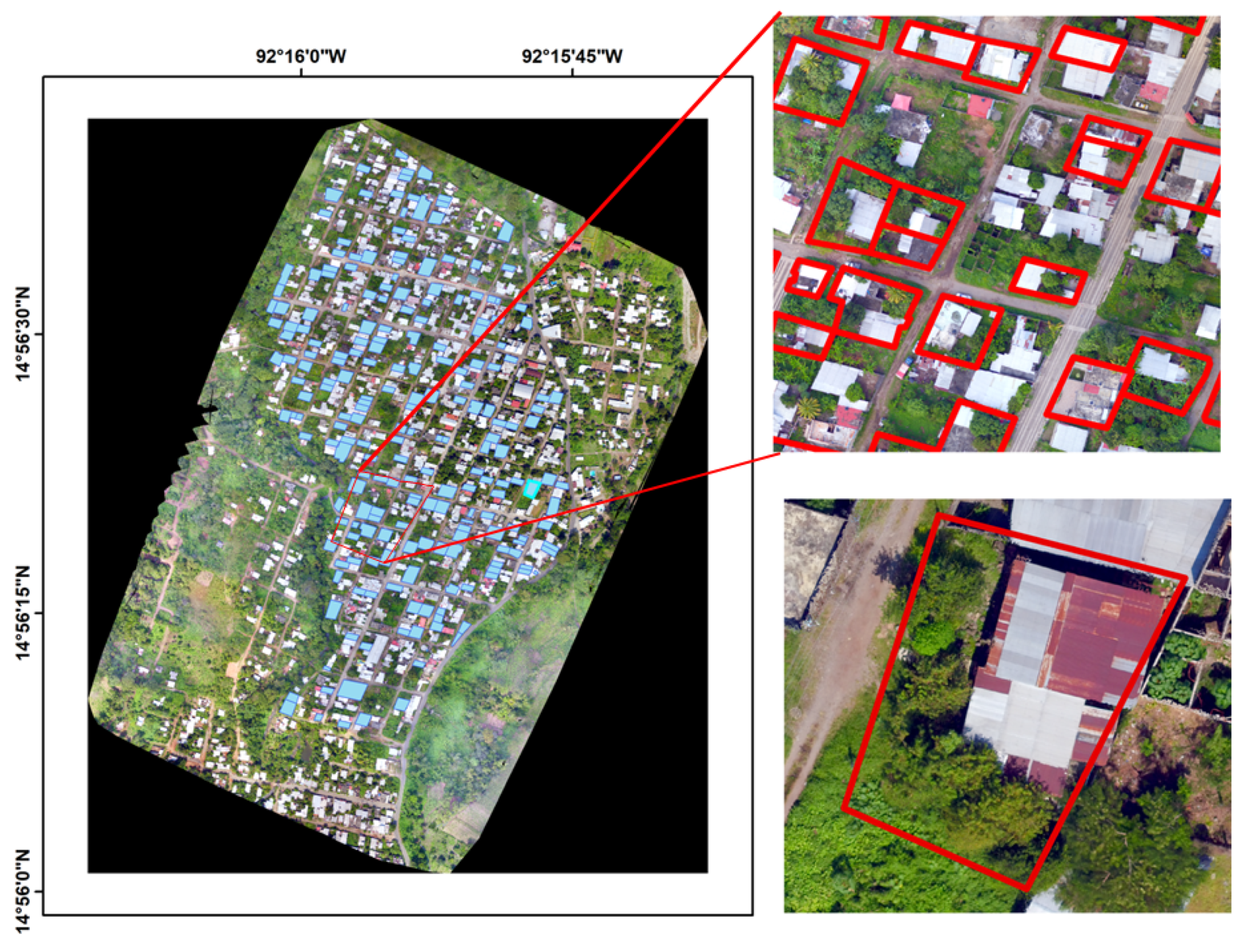
3.1. Study Area

Tapachula is the second-most important city in Chiapas, the economic capital of the state and the main populated center of the Soconusco region. In 2018, it was first, epidemiologically, in cases of dengue, with 876 cases registered, an increase of 188% in relation to 2019. Tapachula city has 217,550 inhabitants and 78,039 houses, and is located on the southern Pacific coast of Chiapas. It has an average annual temperature of 21.7 °C and rainfall of 1000–5000 mm [40]. The climate is warm, humid, and temperate, with a heavy rainy season from May to November. The area of study is El Vergel, a colony in the northwest of Tapachula, with an extension of 433 km 2 (Figure 1). It has an estimated population of 2590 people (residents and workers) in 592 houses. There were 597 inhabitants per km 2 , with an average age of 11 years and an average of seven years of schooling.

3.2. Field Surveys

Surveys were conducted in 216 houses in the El Vergel neighborhood in Tapachula, Chiapas, from 19 November to 5 December 2020 (Figure 1). The surveys were carried out among inhabitants of legal age.
Four household surveys were conducted in El Vergel neighborhood, Tapachula, Chiapas: (a) the Premise Condition Index (PCI, [41]) and the Modified Premise Condition Index ( PCI 2 , [42]), (b) the entomological survey for adults of Ae. aegypti, (c) the entomological survey for larval breeding sites of Ae. aegypti, and (d) a demographic survey. These surveys are described below.

3.2.1. Premise Condition Index (PCI)

This survey consists of nine questions related to the house appearance or house condition, the yard condition, and the degree of shade; the value of this index oscillates in three levels: low, medium, and high [41]. The modified premise condition index (PCI 2 ) was also obtained from this survey, including the yard conditions and the degree of shade, without house conditions [42].

3.2.2. Entomological Survey for Adults of Ae. aegypti

These surveys were carried out once in all rooms of each house for the manual collection of Ae. aegypti at rest by using backpack aspirators [43]; this tool also can collect mosquitoes while flying at 10 or 15 cm from the mouth of the catch container. The mosquito count was done manually in the field and recorded per house. Then, the adult mosquitoes were transported in small cages covered with mash and labeled, one per house, into a cooler to the laboratory. The adults were then identified morphologically, according to [44].

3.2.3. Entomological Survey for Ae. aegypti Breeding Sites

In the same manner, this survey was carried out once and consisted of a visual inspection of each house, looking for all containers that could be holding water to look for eggs, larvae, or pupae of Ae. aegypti, indoor, outdoor, and on roofs of houses when it was possible. A container had eggs, larvae, or pupae of Ae. aegypti was identified as a positive breeding site. The number of eggs, larvae per stage, and pupae per container were counted manually and recorded per house [45].
Ladles, mesh nets, mosquito larvae dippers, and plastic pipettes were used to check each container. The small and medium containers were emptied for larvae and pupae counted, and for the large containers, the personnel used small containers for which all the immature stages of Ae. aegypti were counted by depth until no larvae or pupal activity was observed in the container [45]. The species were identified in the field according to [44]. Previous training was necessary for field personnel to strengthen their knowledge about the vector and fill out the entomological surveys.

3.2.4. Overcrowding

This index was constructed from the demographic and socioeconomic survey applied once to each house. It consists of the number of inhabitants/number of house rooms of 216 houses surveyed.

3.3. Drone Photography and Cartography Construction
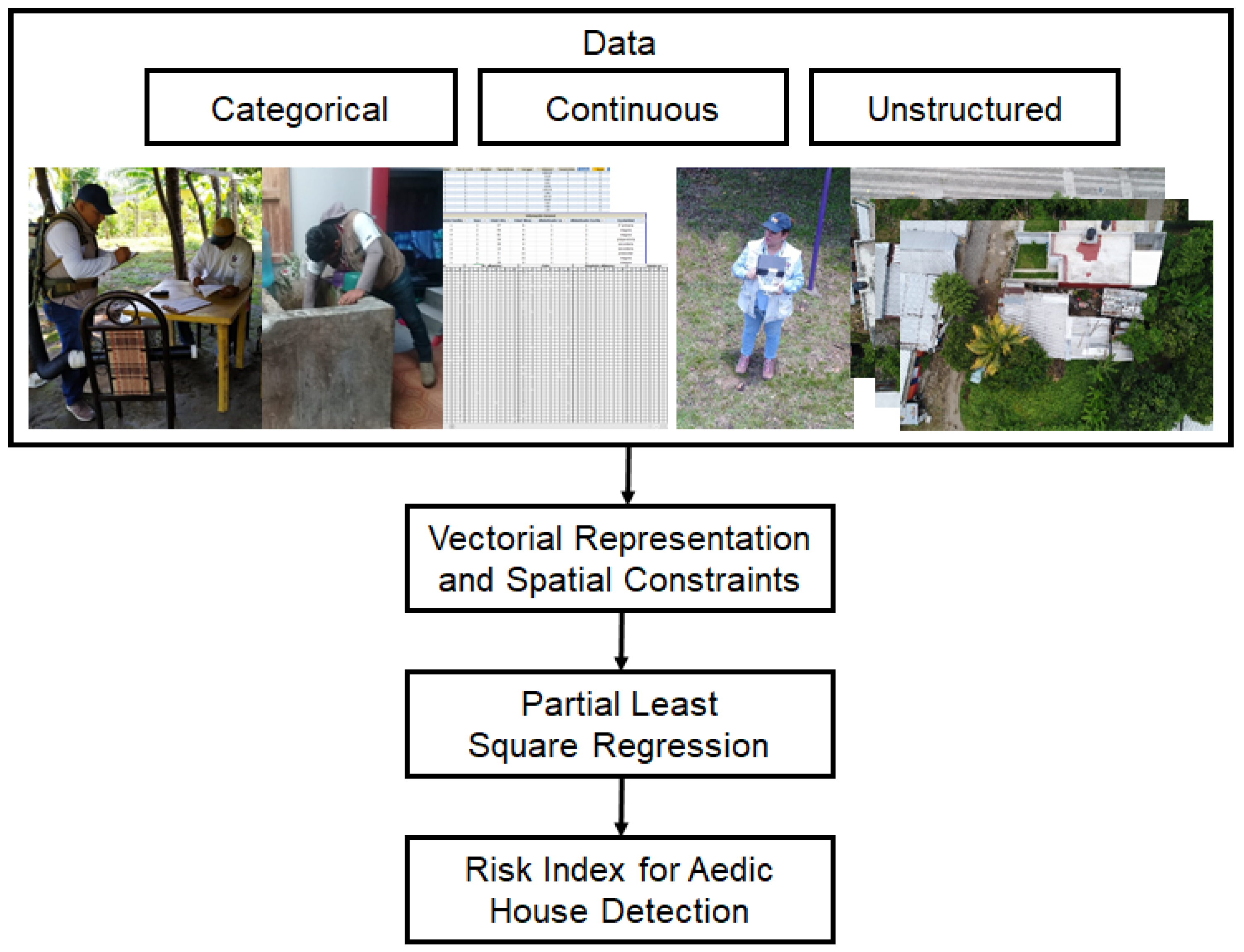
We use a Matrice 600 DJI® RPAS equipment [22] with a high-resolution 16-megapixel X5 optical camera [46] and a MicaSense Rededge® multispectral camera [47] in order to create cartographic products such as orthomosaics, contour lines, housing classification, and vegetation indices (NDVI, GNDVI, NDVIRedEdge, and CIgreen) [10]. The drone flights were made in collaboration with the National Centre for Disaster Prevention of the Mexican Government (CENAPRED) by using the CENAPRED protocols [48] and following the national normative law [49] and manufacturers’ recommendations [22]. The flight plan was carried out by using the PIX4D software [50] which allows flight speed and height variables, camera tilt angle, and overlap between images to be kept constant. All flights were made at 100 m of altitude with a resolution of 2.59 cm/pixel by noon, trying to avoid the shadows [12,51,52], and on the same week of the field surveillance. At the same time, we take drone photographs on RGB by X5 optical camera and on five spectral bands (R, G, B, RedEdge, and NIR) by Micasense® camera.
Once the flight plan is carried out over the study area, photographs captured by the sensor are obtained in JPG format and transferred to the computer for processing. All aerial photographs were processed by using PiX4D [50] software to obtain the georeferenced orthomosaic. These models are created from the process on the point cloud generated by the captured photographs to obtain products such as the orthophoto, digital surface model (DSM), and digital terrain model (DTM) with a spatial resolution of 5 cm. These cartographic products are obtained for both cameras, performing separate processing (Pix4Dmapper version 4.3.31 [53]). Raster data of all structures and vegetation represents the DSM and the development of the geodesic surface represents the DTM. For the classification of vegetation and houses, the RGB orthomosaic was subjected to radiometric calibration by using the ENVI spectral signature library [54] with the empirical line compute (ELC) factors algorithm, and thus it can perform postprocessing on the image, such as supervised classification with the maximum likelihood estimation (MLE) method. The RGB orthomosaic was obtained of the El Vergel neighborhood, where we can see houses, roads, highways, rivers, and trails in detail. Areas with a strong influence of vegetation can be observed, detailing the location of the houses’ roofs or infrastructure, as well as the vegetation types, grass, bushes, and trees of different dimensions (see Figure 1). Once the raster formats were obtained, the processing of polygons that cover the coverage of buildings and vegetation continued. The 216 houses were located in the aforementioned raster. Two types of polygons were digitized in the total area of each house: house coverage by roofs and vegetation coverage by trees. Both were divided into three strata: 1. less than 25%; 2. from 26 to 50%; and 3. more than 50%. Shade cover (ShadeDrone) was based on the building cover (roofs) plus the tree cover per house. The cartography of different vegetation indices (Normalized Difference Vegetation Index (NDVI), Green Normalized Difference Vegetation Index (GNDVI), Normalized Difference Red Edge Index (NDVIre), Green Chlorophyll Index (CIgreen) [55], and tree height cartography) were generated by using the ArcMap software from the raster calculator tool [56] that allows the application of different formulas already estimated previously to obtain them, using as inputs the bands of our multispectral sensor (R-G - B- IR- RE).
Finally, the shapefiles of the houses ( N = 216 ) of El Vergel, Tapachula, Chiapas were individually separated house by house. Subsequently, 100 points were randomly created on the ArcMap® 10.3 platform within each house. Each variable derived from the vegetation indices (NDVIre, GNDVI, NDVI, and CIgreen), DSM, and DTM consisted of an average of 100 points per house. A summary of the variables we consider in our analysis is shown in Table 1. Time photo capture and flight height were allowed the resolution necessary for recording data of the landscape variables for Aedes risk index (Table 1). The UAV photos taken simultaneously with the data recorded through field surveillance reflect the elements found in the field.

3.4. Methodology

Given the data gathered according to Section 3.2, our proposed index is based on two steps (see Figure 2). First, we obtain a vectorial representation of each house included in our study in such a way that we can obtain similarities among them. This step involves an encoding procedure to the raw data, which takes into account the different types of variables we have. In the second step, we obtain the index as a latent variable derived from a particular regression procedure by introducing a dependent variable related to the Ae. aegypti. In the following sections, we describe in detail those steps.

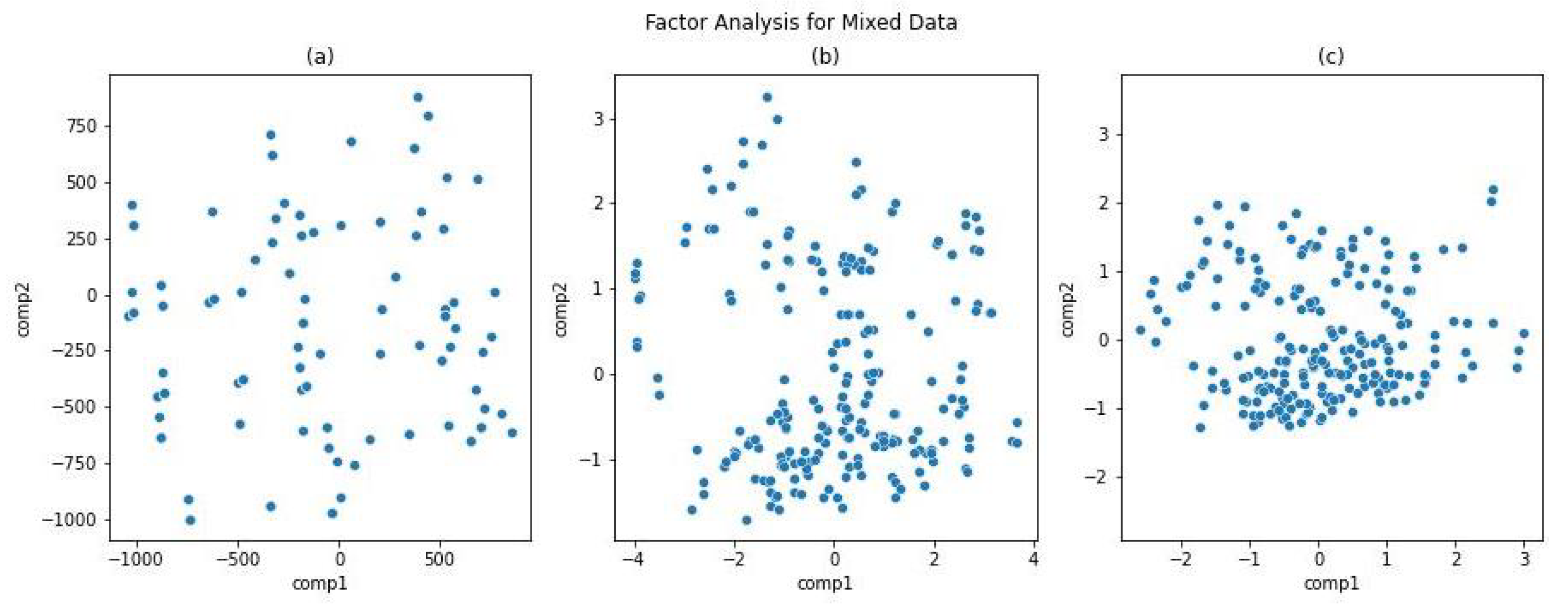
3.4.1. Vectorial Representation of the Data

The methodology we propose to obtain the risk index requires a vectorial representation of the data. In the case of medium- to high-dimensional data, it is recommended that this representation be low dimensional, and therefore, a dimensionality reduction procedure is envolved.
Principal Component Analysis (PCA [57]) and Multiple Correspondence Analysis (MCA [58,59]) are well-known techniques to obtain low-dimensional representations of quantitative and qualitative data, respectively. When we have mixed-type data, i.e., quantitative and qualitative, as in our case, there are some proposals in the literature where, prior to the dimensionality reduction, an encoding procedure is done to one or both types of variables. The simplest encoding procedure is the discretization of the quantitative features by mapping continuous values into predefined intervals (e.g., low, medium, high), in order to obtain a complete categorical dataset; however, valuable information can be ignored, and defining the appropriate intervals can be tricky. It is also possible to obtain a quantitative dataset by introducing dummy variables, where qualitative features are transformed via a one-hot encoding procedure, whereby each category is represented as a binary variable. Although it is a common practice in regression models, several drawbacks have been noted, such as the increase in size of the dataset, and mainly, the multicollinearity problems that can be found [60]. Another approach is to construct a metric space with a similarity measure between pairs of objects defined in such a way that it can handle mixed-type data, such as multidimensional scaling (MDS, [61]) with Gower distance ([62]). Another sophisticated method for encoding mixed-type data based on Shannon entropy has been proposed in [63], where it is shown that the obtained representation can preserve the information in the original data with a memory-efficient procedure, which is particularly useful for big data scenarios (large and high-dimensional datasets). Another popular alternative for low to medium-size datasets, is factor analysis for mixed data (FAMD, [64,65]), which can be viewed as a mix between PCA and MCA. As is noted in [64], FAMD can be obtained by PCA including quantitative variables with a particular metric, which includes the contribution of quantitative and qualitative variables (previously encoded) to the distance between pairs of observations. This is the approach we use in our proposal, and in the next paragraph, we will describe the FAMD methodology following [66].

Factor Analysis for Mixed Data

Let X n × d be our data matrix, with n observations and d = c + q variables, of which c are quantitative and q are qualitative. Now, let us define the encoded data matrices Z C and Z Q for quantitative and qualitative variables, respectively. For quantitative variables, we use the centered-scaled version: Z i j C = ( X i j x ¯ j ) / σ j for j C , where C is the set of quantitative variables. For qualitative variables, Z Q is the so-called complete disjunctive table, which is a multivariate indicator matrix, the rows of which are the concatenation of q one-hot encoding vectors for each q Q , the set of qualitative variables. Suppose that the qth variable has K q categories and K = q K q is the total number of categories for all qualitative variables. Then, Z Q is a matrix of size n × K , with entries Z i k Q = 1 if observation i belongs to the kth category and 0 otherwise, for i = 1 , 2 , , n and k = 1 , 2 , , K . Generally, we use the scaled version of Z Q , where each entry is set to Z i k Q / p k 1 , where p k is the proportion of observations possessing category k. Those transformations give us a new data matrix Z = [ Z C , Z Q ] , with observations z R s , where the dimension of this metric space is s = c + K . For any two observations u , v R s , a weighted norm is defined as u W 2 = u W u , and its corrreponding weighted distance will be d W 2 ( u , v ) = u v W 2 = ( u v ) W ( u v ) .
In order to take into account the two types of variables in the distance defined before, in the standard version of FAMD, the weight matrix is defined as W = diag ( [ 1 c , p ] ) , where 1 c is the vector of ones with length c, and p is the vector of category proportions of length K. The latter implies a weighted scheme on the columns of Z Q when the distance between encoded observations is computed, which together with the scaling defined before, emphasizes the differences between observations with rare categories. However, another weighting scheme is possible, as is noted in [66]. The fitting of the model is similar to PCA on the transformed variables, based on singular value decomposition (SVD), where an additional weighting scheme is applied for the row space of Z by means of B n × n = diag ( 1 n 1 ) ; then, the solution is based on SVD ( B 1 / 2 Z W 1 / 2 ) . See [64] for details.
Similar to PCA and MCA, FAMD gives us low-dimensional representations for variables and observations. In our case, we will only use the representations for observations, which allow us to measure similarities in houses according to their characteristics.

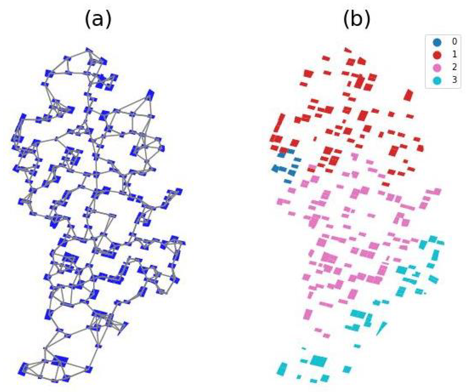
3.4.2. Spatial Constraints

The spatial relationships between the houses in our study are based on their geographic distribution. We used a ML methodology to generate a categorical variable for each house, which we add to the original variables, corresponding to the cluster they belong to, according to a particular clustering structure obtained with a clustering algorithm with spatial constraints. The constraint we used is the contiguity in space, specifying in this way which observations (houses) are considered connected. When we include these connectivities in a clustering algorithm, the observations in a cluster are required not only to be similar to one other according to their covariates, but also to comprise a contiguous set of observations. To this end, we define a connectivity matrix C n × n with entries C i j = 1 if observations i and j are considered contiguous and 0 otherwise. A cluster is then considered contiguous if there is a path between every pair of observations in that cluster, i.e., the subgraph is fully connected. Several classical ML clustering algorithms have been modified to take into account this type of constraint [67,68]. We decided to use an agglomerative hierarchical clustering method adapted to handle connectivity constraints implemented in the module cluster from sklearn package in Python [69]. We chose this method mainly because of its simplicity and the good results that we obtained.

3.4.3. Risk Index with Partial Least Squares

Our proposed index is based on partial least squares regression (PLS, [70,71]). PLS is a class of techniques for modeling the association between blocks of observed variables through latent variables.
Let X ˜ n × p and Y n × t , be the matrices representing a set of independent and dependent variables, respectively, which we assume, are linearly related. PLS aims to find a set of vectors of latent scores { α 1 . , α R } and { ω 1 . , ω R } , which are orthogonal and related to the column space of X ˜ and Y , in such a way that, for any value between 1 and R, this set of vectors span the “most interesting” subspaces of the ranges of both matrices [72]. Taken separately, α r and ω r for r = 1 , , R , can be the PCA solution for X ˜ and Y ; however, the solution of PLS is not accounting for X ˜ X ˜ or Y Y only, but for the cross-covariance X ˜ Y . Let us focus on the first pair of latent scores α 1 and ω 1 . In this case, PLS can be stated as a method to find vectors a and b such that
Cov ( α 1 , ω 1 ) = max a = b = 1 Cov ( X ˜ a , Y b ) .
If a 1 and b 1 are the solution to (1), it can be shown that Cov ( α 1 , ω 1 ) a 1 b 1 is the best rank-one approximation of X ˜ Y in the least-squares sense [72].
In its classical form, the fitting procedure of PLS is based on the nonlinear iterative partial least squares (NIPALS) algorithm [73], which give us the whole set of solutions ( α r , ω r ) and ( a r , b r ) , for r = 1 , , R .
In our study, the data matrix X ˜ n × p is the p –dimensional representation of the original mixed-type dataset obtained with the methodology described in Section 3.4.1. The dependent variable Y is a n × 1 matrix (i.e., a vector). In this case, the solution is given by a particular case of PLS known as PLS1 [71,72].
Our particular interest is the solution given by the first pair of PLS scores, because our proposed index is given by X ˜ a 1 .

4. Results

We performed an extensive set of experiments in order to explore interesting patterns and to select a good model to obtain our proposed index. Those experiments where carried out based on a grid of parameters, which we consider important, and are described on Table 2.
As in any regression-based model, in PLS we can obtain some metrics accounting for its predictive performance; however, it is not our objective (it is very easy to show that a performance metric such as the coefficient of determination, can be artificially “inflated”, resulting in an overfitted model). In our case, we want to take advantage of a unique characteristic of PLS: to construct the best set of latent variables (components) based on the set of factors we obtained with FAMD, which are correlated to our response variable of interest, as we explained in Section 3.4.3. In this sense, we want to exploit the explanatory habilities of PLS, which will allow us to obtain a set of components that can represent all covariates we used (from different sources and types) in a useful way to be considered as a risk index.
Then, our main evaluation criteria was the explained inertia (covariance) obtained with the FAMD procedure according to the P C F A M D variable, and the residuals on log counts of the response variables. Because we have many possible combinations of the parameters, we will not show here those experiments, but many of them can be found as supplementary material to this paper in https://github.com/victorm0202/mosquito_borne_viral_disease_paper.
We observe that the patterns of risk we found are consistent in most of the parameterizations we used, except on those where the model overfits, and we observed also that this tends to occur when P C P L S is high (5 or 6, mainly). In this case, the risk index does not show a particular spatial trend, even when we vary the other parameters.
Based on those experiments, we decided to use the following parameters of our proposed model for the results we will show:
  • P C D r o n e I m a g e : 1
  • n c l u s t : 4
  • k n n : 3
  • P C F A M D : 2
  • P C P L S : 2
obtaining an explained inertia of 0.661 .
Based on this set of parameters, and the geographic distribution of the houses included in our study, we generate a cluster configuration by using agglomerative hierarchical clustering with spatial constraints, as is explained in Section 3.4.2, where we included all independent variables related to the houses of our dataset.
In Figure 3, we show the connectivities induced by C by using the centroids of the polygons defining the houses and the cluster configuration of houses according to four regions. We add a categorical variable to our dataset which represents the region assigned to each house.
We apply FAMD to the complete dataset of independent variables, including that for the region. As was explained in Section 3.4.1, we can obtain low-dimensional representations for variables and observations, but it will be restricted to observations only, because our interest is to have a useful representation for the houses according to all their covariates. Because FAMD is based on MCA and PCA, we can obtain representations based on each type of variable, as we show in Figure 4. For visualization purposes, we show two-dimensional representations of observations based on qualitative variables (Figure 4a), quantitative variables (Figure 4b), and the complete set of variables (Figure 4c), which is our main interest.
We can see that some patterns emerge when we use categorical and continuous variables only, but perhaps it is more clear in the case of continuous variables (Figure 4b), where we can observe a main cluster of houses, and three smaller clusters. Moreover, we can see at least two clusters when we consider the whole set of variables, as is shown in Figure 4c. We tried to explore a little more on this fact by applying k –means clustering considering the 3 PC we get with FAMD and k = 4 clusters. The results are shown in Figure 5. Initially, we wonder if those patterns corresponded to the spatial configuration we found in Figure 3. This was not the case, but we will use the clusters we found with k –means to compare with the results we obtained with the proposed index.
To construct our univariate index with PLS, as we explained in Section 3.4.3, we use different dependent variables Y . In all cases, our index is defined as γ = X ˜ a 1 , a vector of length n, and it corresponds to the first PLS score.
We use univariate and multivariate Y as dependent variables for PLS. The univariate dependent variables are denoted by Y pupae , Y mosquitoes and Y stages . Meanwhile, the multivariate version includes all the previous variables concatenated by columns, resulting in a matrix Y all of size n × 3 .
For visualization purposes, and in order to compare our proposed indices, we show in Figure 6 the bivariate risk index, which corresponds to the first two scores obtained with PLS for each Y . The points represent the houses, and the cluster assigned to each point is the same that we obtained with k –means in the FAMD representation (Figure 5). We observe similar patterns in the FAMD representation and the index obtained; furthermore, we can see that all bivariate indexes in Figure 6 are very similar.
For practical purposes, our proposed index is univariate and, as we said before, corresponds to the first score obtained with PLS, which was scaled between zero and one. In Figure 7 we show the house-level risk index we propose based on PLS for each dependent variable Y defined before. This figure confirms the similarity between all indices.
In addition, we show in Figure 8 the geographic distribution of houses, depicted with polygons, and the risk index for each house. Very interesting patterns can be seen in both Figure 7 and Figure 8. There are some evident peaks of the risk index, which mainly correspond to houses on the periphery of the region of study. This spatial pattern of high-risk houses corresponds to region 3 in Figure 3, and some houses of regions 0 and 1. Houses with low risk can be found in the center of the study region and correspond to the region 2 of Figure 3. The risk increases as we approach the periphery of the region, as can be seen in Figure 8.
The house risk index of less than 0.5 for larvae, pupae, adults, and all stages was in 69.4% (150), 70.4% (152), 71.8% (155), and 70.4% (152) of houses, respectively. The major part of the houses with low risk (less than 0.5) was located in the downtown of the El Vergel neighborhood. The characteristics of this area are different from the rest of the dwellings in several aspects: they have concrete slab roofs and tile floors, better-quality services, and less tree cover, among other things, as opposed to the peripheral houses, which are characterized by more vegetation cover, sheet metal roofs, deficiency in the provision of services and constant population movement. This may represent a greater risk for dengue transmission in these particular areas. For all of the above, the generated maps can be added to the layers of geographic information that strengthen decision making on mosquito prevention and control measures in the area. They can permit direct mosquito control activities for those houses with high risk for Ae. aegypti in different life-cycle stages with adequate activities can involve community participation.

5. Discussion

The use of new technologies such as UAV have proven useful in supporting the implementation of entomological surveillance strategies for emerging and reemerging diseases. For malaria, the use of drones has allowed vegetation to be associated with the abundance and presence of the vector. On the other hand, methodology for monitoring and identifying breeding sites of Ae. aegypti mosquitoes has recently been reported.
The traditional entomological surveillance was carried out in homes by the Vector Control Program in Mexico and used entomological indices. The house (premises), index (percentage of houses infested with Ae. aegypti, larvae and/or pupae), container index (percentage of water-holding containers infested with Ae. aegypti larvae and/or pupae), and the Breteau index (number of positive containers per 100 houses recorded) [74], showed little relationship to adult densities. In some situations, their values were not associated with cases in the locality [75,76,77]. Likewise, the national dengue program uses some indices to determine risk areas where the vector develops. One of them is the Premise Condition Index (PCI). This index considers the house’s appearance, the shade, and the disorder in the patio of the dwellings to determine the degree of risk in the dwelling in the presence or absence of the vector [42]. In [42], the potential of aerial surveillance for identifying breeding sites of Ae. aegypti was demonstrated two decades ago. Satellite aerial photographs intended to identify high-altitude breeding and resting sites of Ae. aegypti in residential areas were compared with the modified Housing Condition Index (PCI 2 ) application [41] as a rapid assessment technique within the dwellings. However, that was limited to the resolution of the images and could not identify small elements of backyards. Nevertheless, the satellite images are taken at different seasons, daily times, and camera angles, which does not allow the precise association of the environmental variables related to the Ae. aegypti house biological cycle. In this study, the UAV photos were taken at 100 m, at approximately noon, and simultaneously with house surveys [12,51,52], making it possible to associate the vector’s biological activity with landscape elements because it allows us to determine them precisely and according to the field data record. The dengue mosquito vector Ae. aegypti has expanded its distribution, as the mosquitoes have gradually adapted to climatic and environmental conditions, leading to a change in the epidemiology of viral diseases, facilitating their establishment in new ecozones inhabited by immunologically naive human populations [78]. Numerous research groups have generated evidence on the factors that facilitate vector mosquitoes’ different life-cycle stages and that are associated with the increase in their populations [34] and disease transmission [79,80]. In addition to the scientific evidence, health programs must know the riches of other technologies to obtain high-resolution images that can help understand the vector-borne diseases (VBD) complex, dynamic, and multifactorial scenarios.
Although dengue and mosquito programs have indices and technological tools that can help understand the mosquito population dynamics, the role of UAVs as a newborn technology can help build a house index more robust that can permit the anticipation of the increase in the mosquito population in health programs.
The national dengue program needs a robust concept to determine an “aedic house” that can have characteristics for allowing Ae. aegypti life cycles. We approach the simultaneity of UAV high-resolution images with field surveillances; data can also be defined, taking into account different types of variables related not only to the dwelling but also population–socioeconomic and other characteristics related to the landscape, such as coverage, type of vegetation present, and topography. Due to the fact that most of the UAV studies have been made on simulation scenarios, the contributions of this study demonstrate the utility of UAVs in obtaining urban landscape data for building a strong, flexible, and robust risk index, the methodology of which can be adapted to different places on different socioeconomic neighbor levels in urban or semiurban areas.
Our model contemplates different types and natures of variables related to the immediate landscape of each house visited, including those made through specialized cartography by aerial images, such as the vegetation present through the coverage and height of trees. The vegetation indices that consider both the greenness and the plant density of the species and values of the digital surface model were included, representing all the elevations present on the surface, land, infrastructure, and vegetation. The plant species present, their height, and their foliage will affect the local temperature and wind speed due to the effect of shadows projected on the various surfaces. Indeed, evapotranspiration is the effect of evaporative cooling of the water that plants transpire. Another small contribution is due to soil moisture [81]. In addition, consider field survey data as the premise condition index [41], the modified house condition index [42], and the number of positive breeding sites for Ae. aegypti, as an indirect measure of the characteristics of the houses that allow them to offer conditions that facilitate the life cycle of mosquitoes and oviposition [82,83,84] and the overcrowding index, as a measure of the human population density can act, among other things, as one of the factors for the female mosquitoes to move in search of food sources [85]. The flight height is crucial to obtain the optimal resolution for identifying the landscape elements according to different scenarios and depends on the elements or object size needed to identify the landscape. It is specific to the research question. However, it is crucial to know the flight area—in urban environments, to avoid high obstacles such as telecommunications or wi-fi antennas, buildings, or tall infrastructure, and in rural and semirural environments, mainly to avoid tall trees. An evaluation was carried out to determine the best flight height for detecting and identifying specific plant communities. They found that the NDVI orthophotograph’s best flight height to identify tolares of P a r a s t r e p h i a l e p i d o p h i l l a was 25 m, followed by 50 m [86]. An optimum flight height for our study purposes was 100 m. For operational purposes, we recommend flights of 80 to 100 m. Moreover, we recommended following the national regulations for security flights. Another important flight issue is photo capture time, which should be at noon, to avoid shadows limiting the object or element detection and identification [12,52]. As dependent variables, all the immature stages of female and male Ae. aegypti mosquitoes that could explain the model were included and made simultaneous with the UAV flights.
Nowadays, there is an evident trend in the ML research community to use data from different sources in order to propose useful models for many phenomena of interest, and entomological surveillance and public health in general are not an exception. In addition to the variables coming from specialized cartography by aerial images explained before, we include several variables coming from field and household surveys (Section 3.2). Certainly, there could be many advantages to incorporating more information from many sources, because more information could enrich our knowledge of the phenomenon we are interested in, and arguably, could improve the model we used for solving some specific task. However, it is very important to pay attention to the way this information is used by our models, especially when different structures are present, giving us mixed-type variables. We think the latter is crucial, particularly for models in which a distance function among objects (houses, in our case) is involved, as is the case of ML-related models. This is because not all distance functions are capable of representing differences between objects with mixed-type data. Consider for example, the Euclidean distance, which is used by default in most of the supervised and nonsupervised ML algorithms, and is aimed at continuous (real-valued) variables; then, if we use a model based on Euclidean distance for categorical or mixed-type data, the results and conclusions we obtain with this model, may not be correct. In our proposed index, we take into account the different types of variables by using an efficient encoding procedure which gives us a shared metric space with a corresponding norm capable of representing distances between any two objects taking into account the two types of input variables we used, and we think this is one of our main contributions, given that similar works reported in the literature [38,39] leave unclear the way by which the mixed input data (categorical and continuous) are managed, or the distance function they used. Although in these works the model takes into account the characteristics (socioeconomic, climate change, dengue knowledge, and landscape factors) of a house as input and returns the prediction of the mosquito to abundance (high or low), our model takes into account the characteristics (environmental, demographic, and socioeconomic) of a house and its spatial relationship with other houses to predict the risk index for being classified as an “aedic” house. In addition, our implementation was carried out with open-source software.
Moreover, in our study, the El Vergel neighborhood presented conditions that determined, for most of the houses surveyed, a premise condition index with a medium risk level, which does not allow focusing prevention and control actions of vectors at the housing and block level in the area. Mexico’s southern border has a wide diversity of ecotones, socioeconomic levels, climates, and a constant movement of migratory groups. The models must be adapted to the particular conditions of the endemic region under study. There is no ideal formula but a series of steps to determine which variables offer greater predictive value for a given area. New spatial analysis tools and mathematical models are fundamental methods in vector control activities [87], and even a multidisciplinary group for analyzing it. In addition, the mapping and spatial modeling technologies and methodologies need to increase affordability for use in public health [88], especially in endemic areas that require certainty, coverage, and opportunity. Predictive models can be used for decision making in preventing various arboviruses transmitted by Aedes in urban and semiurban endemic areas based on the evidence of overlapping Aedes-borne diseases (dengue, chikungunya, and zika) within geographic hotspots [89]. This methodology can adapt the model to the different regions of our country. This flexibility is allowed mainly by the availability of real-time information provided by drones, one of its most important contributions.
Our model can be improved in many ways, which we mention as development and future work. It is already advisable to have information at different times of the year to strengthen our model. Tapachula is an area where the dry and rainy seasons are strongly marked and determine a contrast in, at least, the availability and type of breeding sites where the vector develops. Likewise, it is necessary to validate the model in different neighborhoods of the municipality of Tapachula, where the conditions of the houses vary mainly depending on their socioeconomic level. Moreover, it is in our interest to explore some adaptations of PLS for count data, because it is not naturally designed to predict this kind of data, and compare with the log-counts approach. We advise exploring artificial intelligence methods, such as deep neural networks, to detect interesting objects (e.g., mosquito breeding sites) from the UAV images. Although there have been some attempts to use those methods, such as convolutional neural networks [90,91] for aerial surveillance of mosquitoes’ oviposition [52], our aim is to use state-of-the-art, real-time object-detection methodologies, such as YOLO [92] and its different versions [93,94,95], and also, to explore methods based on geographic object-based image analysis (GEOBIA) [96,97] to develop tools for image segmentation and labeling to create training datasets, in order to expand the information of the model in real time, and to strengthen the community’s perception of new technologies as is suggested by [98,99]. This helps to strengthen the timeliness and fidelity of entomological and epidemiological, sociodemographic, and environmental data.

6. Conclusions

This study shows that the use of UAVs can be incorporated into vector surveillance and control strategies, providing spatial and temporal data of the landscape components that allow dengue vectors to continue transmitting the disease in real time. On the other hand, the model based on ML and multivariate statistical techniques, proposed in this study to estimate the risk of dengue transmission, demonstrates high reliability in identifying high-risk areas within the study locality and managing control activities specifically.

Supplementary Materials

The following supporting information can be downloaded at: https://github.com/victorm0202/mosquito_borne_viral_disease_paper (accessed on 30 November 2022).

Author Contributions

Conceptualization, V.M.-S., K.M.V.-D. and R.D.-L.; methodology, V.M.-S., K.M.V.-D. and R.D.-L.; software, V.M.-S., F.J.H.-L. and D.A.M.-L.; validation, V.M.-S., K.M.V.-D. and R.D.-L.; formal analysis, V.M.-S. and F.J.H.-L.; investigation, V.M.-S., K.M.V.-D., F.J.H.-L., D.A.M.-L., R.D.-L. and G.G.-F.; resources, V.M.-S., K.M.V.-D., D.A.M.-L. and F.J.H.-L.; data curation, V.M.-S., K.M.V.-D., D.A.M.-L. and F.J.H.-L.; writing—original draft preparation, V.M.-S., K.M.V.-D., F.J.H.-L. and D.A.M.-L.; writing—review and editing, R.D.-L. and G.G.-F.; visualization, V.M.-S., K.M.V.-D., F.J.H.-L. and D.A.M.-L.; supervision, R.D.-L. and G.G.-F.; project administration, R.D.-L. and G.G.-F.; funding acquisition, R.D.-L. and G.G.-F. All authors have read and agreed to the published version of the manuscript.

Funding

This research was carried out with the support of four institutions of the Mexican government. (1) The vector control program of the health services of Chiapas for entomological activities in the field, (2) CENAPRED research group to carry out the flight of the drones and elaboration of cartography, (3) Group of CIMAT researchers for the elaboration of mathematical models and (4) CRISP/INSP technical personnel for the application of sociodemographic and Premise Condition Index surveys and researches for a biological point of view of results.

Institutional Review Board Statement

Ethics and Research Committee approval of Distrito Sanitario #7, Chiapas Health Services.

Informed Consent Statement

Informed consent was obtained from all subjects involved in the study.

Data Availability Statement

Not applicable.

Acknowledgments

We greatly appreciate the householders, authorities of El Vergel, Tapachula, Chiapas, and the authorities of Distrito Sanitario #7 of Chiapas Health Services for the facilities provided in this study. The authors also acknowledge the National Disaster Prevention Center of the Mexican Government for the UAVs flights, photographs, and cartography used in this study.

Conflicts of Interest

The authors declare no conflict of interest.

References

  1. Nex, F.; Remondino, F. UAV for 3D mapping applications: A review. Appl. Geomat. 2014, 6, 1–15. [Google Scholar] [CrossRef]
  2. Eskandari, R.; Mahdianpari, M.; Mohammadimanesh, F.; Salehi, B.; Brisco, B.; Homayouni, S. Meta-analysis of Unmanned Aerial Vehicle (UAV) Imagery for Agro-environmental Monitoring Using Machine Learning and Statistical Models. Remote Sens. 2020, 12, 3511. [Google Scholar] [CrossRef]
  3. Rojas Viloria, D.; Solano Charris, E.L.; Muñoz Villamizar, A.; Montoya Torres, J.R. Unmanned aerial vehicles/drones in vehicle routing problems: A literature review. Int. Trans. Oper. Res. 2021, 28, 1626–1657. [Google Scholar] [CrossRef]
  4. Bendig, J.; Bolten, A.; Bareth, G. Introducing a Low-Cost Mini-Uav for-and Multispectral-Imaging. ISPRS Int. Arch. Photogramm. Remote Sens. Spat. Inf. Sci. 2012, 39B1, 345–349. [Google Scholar] [CrossRef] [Green Version]
  5. Landau, K.; Van Leeuwen, W. Fine Scale Spatial Urban Land Cover Factors Associated with Adult Mosquito Abundance and Risk in Tucson, Arizona. J. Vector Ecol. J. Soc. Vector Ecol. 2012, 37, 407–418. [Google Scholar] [CrossRef]
  6. Ivosevic, B.; Han, Y.G.; Kwon, O. Calculating coniferous tree coverage using unmanned aerial vehicle photogrammetry. J. Ecol. Environ. 2017, 41, 1–8. [Google Scholar] [CrossRef] [Green Version]
  7. Robb, C.; Hardy, A.; Doonan, J.H.; Brook, J. Semi-Automated Field Plot Segmentation From UAS Imagery for Experimental Agriculture. Front. Plant Sci. 2020, 11, 591886. [Google Scholar] [CrossRef]
  8. González-Jorge, H.; Martínez-Sánchez, J.; Bueno, M.; Arias, P. Unmanned Aerial Systems for Civil Applications: A Review. Drones 2017, 1, 2. [Google Scholar] [CrossRef] [Green Version]
  9. Hassanalian, M.; Abdelkefi, A. Classifications, applications, and design challenges of drones: A review. Prog. Aerosp. Sci. 2017, 91, 99–131. [Google Scholar] [CrossRef]
  10. Fornace, K.M.; Drakeley, C.J.; William, T.; Espino, F.; Cox, J. Mapping infectious disease landscapes: Unmanned aerial vehicles and epidemiology. Trends Parasitol. 2014, 30, 514–519. [Google Scholar] [CrossRef]
  11. Hardy, A.; Makame, M.; Cross, D.; Majambere, S.; Msellem, M. Using low-cost drones to map malaria vector habitats. Parasites Vectors 2017, 10, 1. [Google Scholar] [CrossRef] [PubMed] [Green Version]
  12. Valdez-Delgado, K.M.; Moo-Llanes, D.A.; Danis-Lozano, R.; Cisneros-Vázquez, L.A.; Flores-Suarez, A.E.; Ponce-García, G.; Medina-De la Garza, C.E.; Díaz-González, E.E.; Fernández-Salas, I. Field effectiveness of drones to identify potential Aedes aegypti breeding sites in household environments from Tapachula, a dengue-endemic city in southern Mexico. Insects 2021, 12, 663. [Google Scholar] [CrossRef] [PubMed]
  13. Haas-Stapleton, E.; Barretto, M.; Castillo, E.; Clausnitzer, R.; Ferdan, R. Assessing Mosquito Breeding Sites and Abundance Using An Unmanned Aircraft. J. Am. Mosq. Control. Assoc. 2019, 35, 228–232. [Google Scholar] [CrossRef] [PubMed] [Green Version]
  14. Johnson, B.J.; Manby, R.; Devine, G.J. Performance of aerial Bacillus thuringiensis var. israelensis applications in mixed saltmarsh-mangrove systems and use of affordable unmanned aerial systems to identify problematic levels of canopy cover. bioRxiv 2020. [Google Scholar] [CrossRef]
  15. Lorenz, C.; Castro, M.C.; Trindade, P.M.P.; Nogueira, M.L.; de Oliveira Lage, M.; Quintanilha, J.A.; Parra, M.C.; Dibo, M.R.; Fávaro, E.A.; Guirado, M.M.; et al. Predicting Aedes aegypti infestation using landscape and thermal features. Sci. Rep. 2020, 10, 21688. [Google Scholar] [CrossRef]
  16. Markwardt, R.; Sorosjinda-Nunthawarasilp, P. Innovations in the Entomological Surveillance of Vector-Borne Diseases; Cambridge Scholars Publisher: Cambridge, UK, 2021. [Google Scholar]
  17. Wilke, A.B.B.; Vasquez, C.; Carvajal, A.; Moreno, M.; Fuller, D.O.; Cardenas, G.; Petrie, W.D.; Beier, J.C. Urbanization favors the proliferation of Aedes aegypti and Culex quinquefasciatus in urban areas of Miami-Dade County, Florida. Sci. Rep. 2021, 11, 22989. [Google Scholar] [CrossRef]
  18. de Jesús Crespo, R.; Rogers, R.E. Habitat Segregation Patterns of Container Breeding Mosquitos: The Role of Urban Heat Islands, Vegetation Cover, and Income Disparity in Cemeteries of New Orleans. Int. J. Environ. Res. Public Health 2022, 19, 245. [Google Scholar] [CrossRef]
  19. Tsuda, Y.; Suwonkerd, W.; Chawprom, S.; Prajakwong, S.; Takagi, M. Different spatial distribution of Aedes aegypti and Aedes albopictus along an urban-rural gradient and the relating environmental factors examined in three villages in northern Thailand. J. Am. Mosq. Control. Assoc. 2006, 22, 222–228. [Google Scholar] [CrossRef]
  20. Vásquez-Trujillo, A.; Cardona, D.; Segura Cardona, A.; Camara, D.; Alves-Honório, N.; Parra-Henao, G. House-Level Risk Factors for Aedes aegypti Infestation in the Urban Center of Castilla la Nueva, Meta State, Colombia. J. Trop. Med. 2021, 2021, 12. [Google Scholar] [CrossRef]
  21. Liu, M.; Wang, X.; Zhou, A.; Fu, X.; Ma, Y.; Piao, C. UAV-YOLO: Small Object Detection on Unmanned Aerial Vehicle Perspective. Sensors 2020, 20, 2238. [Google Scholar] [CrossRef]
  22. DJI. Matrice 600®. Available online: https://www.dji.com/mx/downloads/products/matrice600 (accessed on 19 October 2019).
  23. Thibbotuwawa, A.; Bocewicz, G.; Nielsen, P.; Banaszak, Z. Unmanned aerial vehicle routing problems: A literature review. Appl. Sci. 2020, 10, 4504. [Google Scholar] [CrossRef]
  24. Diario Oficial de la Federación. NORMA Oficial Mexicana NOM-032-SSA2-2014, Para la Vigilancia Epidemiológica, Promoción, Prevención y Control de las Enfermedades Transmitidas por Vectores. 2015. Available online: https://www.dof.gob.mx/nota_detalle.php?codigo=5389045&fecha=16/04/2015 (accessed on 18 April 2019).
  25. Hardy, A.; Proctor, M.; MacCallum, C.; Shawe, J.; Abdalla, S.; Ali, R.; Abdalla, S.; Oakes, G.; Rosu, L.; Worrall, E. Conditional trust: Community perceptions of drone use in malaria control in Zanzibar. Technol. Soc. 2022, 68, 101895. [Google Scholar] [CrossRef] [PubMed]
  26. Carrillo-Larco, R.; Moscoso-Porras, M.; Taype-Rondan, A.; Ruiz-Alejos, A.; Bernabe-Ortiz, A. The use of unmanned aerial vehicles for health purposes: A systematic review of experimental studies. Glob. Health Epidemiol. Genom. 2018, 3, e13. [Google Scholar] [CrossRef] [PubMed]
  27. Laksham, K.B. Unmanned aerial vehicle (drones) in public health: A SWOT analysis. J. Fam. Med. Prim. Care 2019, 8, 342–346. [Google Scholar] [CrossRef] [PubMed]
  28. Williams, G.M.; Wang, Y.; Suman, D.S.; Unlu, I.; Gaugler, R. The development of autonomous unmanned aircraft systems for mosquito control. PLoS ONE 2020, 15, e0235548. [Google Scholar] [CrossRef]
  29. Faraji, A.; Haas-Stapleton, E.; Sorensen, B.; Scholl, M.; Goodman, G.; Buettner, J.; Schon, S.; Lefkow, N.; Lewis, C.; Fritz, B.; et al. Toys or Tools? Utilization of Unmanned Aerial Systems in Mosquito and Vector Control Programs. J. Econ. Entomol. 2021, 114, 1896–1909. [Google Scholar] [CrossRef]
  30. Bouyer, J.; Culbert, N.J.; Dicko, A.H.; Pacheco, M.G.; Virginio, J.; Pedrosa, M.C.; Garziera, L.; Pinto, A.T.M.; Klaptocz, A.; Germann, J.; et al. Field performance of sterile male mosquitoes released from an uncrewed aerial vehicle. Sci. Robot. 2020, 5, eaba6251. [Google Scholar] [CrossRef]
  31. Marina, C.; Liedo, P.; Bond, G.; Osorio, A.; Valle Mora, J.; Angulo, R.; Gomez-Simuta, Y.; Fernandez Salas, I.; Dor, A.; Williams, T. Comparison of Ground Release and Drone-Mediated Aerial Release of Aedes aegypti Sterile Males in Southern Mexico: Efficacy and Challenges. Insects 2022, 13, 347. [Google Scholar] [CrossRef]
  32. Carrasco-Escobar, G.; Manrique, E.; Ruiz-Cabrejos, J.; Saavedra, M.; Alava, F.; Bickersmith, S.; Prussing, C.; Vinetz, J.M.; Conn, J.E.; Moreno, M.; et al. High-accuracy detection of malaria vector larval habitats using drone-based multispectral imagery. PLoS Neglected Trop. Dis. 2019, 13, 1–24. [Google Scholar] [CrossRef] [Green Version]
  33. Aragão, F.V.; Cavicchioli Zola, F.; Nogueira Marinho, L.H.; de Genaro Chiroli, D.M.; Braghini Junior, A.; Colmenero, J.C. Choice of unmanned aerial vehicles for identification of mosquito breeding sites. Geospatial Health 2020, 15, 92–100. [Google Scholar] [CrossRef]
  34. Sallam, M.F.; Fizer, C.; Pilant, A.N.; Whung, P.Y. Systematic Review: Land Cover, Meteorological, and Socioeconomic Determinants of Aedes Mosquito Habitat for Risk Mapping. Int. J. Environ. Res. Public Health 2017, 14, 1230. [Google Scholar] [CrossRef] [PubMed] [Green Version]
  35. Estallo, E.; Sangermano, F.; Grech, M.; Ludueña-Almeida, F.; Frías-Cespedes, M.; Ainete, M.; Almirón, W.; Livdahl, T. Modelling the distribution of the vector Aedes aegypti in a central Argentine city: Modelling Aedes aegypti distribution. Med. Vet. Entomol. 2018, 32, 451–461. [Google Scholar] [CrossRef] [PubMed] [Green Version]
  36. Obenauer, J.; Joyner, T.A.; Harris, J.B. The importance of human population characteristics in modeling Aedes aegypti distributions and assessing risk of mosquito-borne infectious diseases. Trop. Med. Health 2017, 45, 1–9. [Google Scholar] [CrossRef] [PubMed] [Green Version]
  37. Cianci, D.; Hartemink, N.; Ibáñez-Justicia, A. Modelling the potential spatial distribution of mosquito species using three different techniques. Int. J. Health Geogr. 2015, 14, 10. [Google Scholar] [CrossRef] [PubMed] [Green Version]
  38. Chen, S.; Whiteman, A.; Li, A.; Rapp, T.; Delmelle, E.; Chen, G.; Brown, C.L.; Robinson, P.; Coffman, M.J.; Janies, D.; et al. An operational machine learning approach to predict mosquito abundance based on socioeconomic and landscape patterns. Landsc. Ecol. 2019, 34, 1295–1311. [Google Scholar] [CrossRef]
  39. Rahman, M.S.; Pientong, C.; Zafar, S.; Ekalaksananan, T.; Paul, R.E.; Haque, U.; Rocklöv, J.; Overgaard, H.J. Mapping the spatial distribution of the dengue vector Aedes aegypti and predicting its abundance in northeastern Thailand using machine-learning approach. One Health 2021, 13, 100358. [Google Scholar] [CrossRef]
  40. INEGI. Censo de Población y Vivienda 2010. Website. 2010. Available online: https://www.inegi.org.mx/programas/ccpv/2010/ (accessed on 18 October 2022).
  41. Tun-Lin, W.; Kay, B.H.; Barnes, A. The Premise Condition Index: A Tool for Streamlining Surveys of Aedes aegypti. Am. J. Trop. Med. Hyg. 1995, 53, 591–594. [Google Scholar] [CrossRef]
  42. Moloney, J.; Skelly, C.; Weinstein, P.; Maguire, M.; Ritchie, S.R. Domestic Aedes aegypti breeding site surveillance: Limitations of remote sensing as a predictive surveillance tool. Am. J. Trop. Med. Hyg. 1998, 59, 261–264. [Google Scholar] [CrossRef] [Green Version]
  43. Silver, J. Mosquito Ecology: Field Sampling Methods; SpringerLink: Springer e-Books; Springer: Dordrecht, The Netherlands, 2008. [Google Scholar]
  44. Darsie, R.; Ward, R.; Chang, C.; Litwak, T. Identification and Geographical Distribution of the Mosquitoes of North America, North of Mexico; University Press of Florida: Gainesville, FL, USA, 2016. [Google Scholar]
  45. Arredondo-Jimenez, J.I.; Valdez-Delgado, K.M. Aedes aegypti pupal/demographic surveys in southern Mexico: Consistency and practicality. Ann. Trop. Med. Parasitol. 2006, 100, 17–32. [Google Scholar] [CrossRef]
  46. DJI. Zenmuse X5®. Available online: https://www.dji.com/mx/zenmuse-x5/info#specs (accessed on 10 October 2019).
  47. Mica Sense Inc. Red Edge®. 2019. Available online: https://support.micasense.com/hc/en-us/articles/115003537673-RedEdge-M-User-Manual-PDF- (accessed on 10 October 2019).
  48. CENAPRED. Centro Nacional de Prevención de Desastres. Website. 2022. Available online: https://www.gob.mx/cenapred/ (accessed on 18 October 2022).
  49. Diario Oficial de la Federación. NORMA Oficial Mexicana NOM-107-SCT3-2019, Que Establece los Requerimientos para Operar un Sistema de Aeronave Pilotada a Distancia (RPAS) en el Espacio aéreo Mexicano. 2019. Available online: http://www.dof.gob.mx/normasOficiales/8006/sct11_C/sct11_C.html (accessed on 15 April 2022).
  50. Pix4D. Capture®. 2019. Available online: https://www.pix4d.com/es/producto/pix4dcapture (accessed on 15 October 2019).
  51. Suduwella, C.; Amarasinghe, A.; Niroshan, L.; Elvitigala, C.; De Zoysa, K.; Keppetiyagama, C. Identifying Mosquito Breeding Sites via Drone Images. In Proceedings of the 3rd Workshop on Micro Aerial Vehicle Networks, Systems, and Applications (DroNet ’17), Niagara Falls, NY, USA, 23 June 2017; Association for Computing Machinery: New York, NY, USA, 2017; pp. 27–30. [Google Scholar] [CrossRef]
  52. Case, E.; Shragai, T.; Harrington, L.; Ren, Y.; Morreale, S.; Erickson, D. Evaluation of unmanned aerial vehicles and neural networks for integrated mosquito management of Aedes albopictus (Diptera: Culicidae). J. Med. Entomol. 2020, 57, 1588–1595. [Google Scholar] [CrossRef]
  53. Pix4D. Mapper®. 2019. Available online: https://www.pix4d.com/es/centro-de-descarga (accessed on 2 December 2019).
  54. L3HARRIS GEOSPATIAL. Getting Started with ENVI. Website. 2022. Available online: https://www.l3harrisgeospatial.com/docs/GettingStartedWithENVI.html (accessed on 20 October 2022).
  55. Díaz, J. Estudios de índices de Vegetación a Partir de Imágenes Aéreas Tomadas Desde RPAS y Aplicaciones de estos a la Agricultura de Precisión. Master’s Thesis, Universidad Complutense de Madrid, Madrid, Spain, 2015. [Google Scholar]
  56. ArcGIS. Raster Calculator. Website. 2022. Available online: https://desktop.arcgis.com/en/arcmap/latest/tools/spatial-analyst-toolbox/raster-calculator.htm (accessed on 20 October 2022).
  57. Jolliffe, I. Principal Component Analysis; Springer: Berlin, Germany, 1986. [Google Scholar]
  58. Greenacre, M.; Blasius, J. Multiple Correspondence Analysis and Related Methods; Chapman & Hall/CRC Statistics in the Social and Behavioral Sciences; CRC Press: Boca Raton, FL, USA, 2006. [Google Scholar]
  59. Izenman, A.J. Modern Multivariate Statistical Techniques: Regression, Classification, and Manifold Learning; Springer: Berlin, Germany, 2008. [Google Scholar]
  60. Garg, A.; Tai, K. Comparison of regression analysis, artificial neural network and genetic programming in handling the multicollinearity problem. In Proceedings of the 2012 Proceedings of International Conference on Modelling, Identification and Control, Wuhan, China, 24–26 June 2012; pp. 353–358. [Google Scholar]
  61. Borg, I.; Groenen, P. Modern Multidimensional Scaling: Theory and Applications; Springer: Berlin, Germany, 2005. [Google Scholar]
  62. Gower, J.C. A General Coefficient of Similarity and Some of Its Properties. Biometrics 1971, 27, 857–871. [Google Scholar] [CrossRef]
  63. Lopez-Arevalo, I.; Aldana-Bobadilla, E.; Molina-Villegas, A.; Galeana-Zapién, H.; Muñiz-Sanchez, V.; Gausin-Valle, S. A Memory-Efficient Encoding Method for Processing Mixed-Type Data on Machine Learning. Entropy 2020, 22, 1391. [Google Scholar] [CrossRef] [PubMed]
  64. Pagès, J. Multiple Factor Analysis by Example Using R; Chapman & Hall/CRC The R Series; Taylor & Francis: Boca Raton, FL, USA, 2014. [Google Scholar]
  65. Pagès, J. Analyse factorielle de données mixtes. Rev. Stat. AppliquÉe 2004, 52, 93–111. [Google Scholar]
  66. Davidow, M.B.; Matteson, D. Factor Analysis of Mixed Data for Anomaly Detection. arXiv 2020, arXiv:abs/2005.12129. [Google Scholar] [CrossRef]
  67. Murtagh, F. A Survey of Algorithms for Contiguity-constrained Clustering and Related Problems. Comput. J. 1985, 28, 82–88. [Google Scholar] [CrossRef] [Green Version]
  68. Wagstaff, K.; Cardie, C.; Rogers, S.; Schrödl, S. Constrained K-Means Clustering with Background Knowledge. In Proceedings of the Eighteenth International Conference on Machine Learning ( ICML ’01), San Francisco, CA, USA, 28 June–1 July 2001; Morgan Kaufmann Publishers Inc.: San Francisco, CA, USA, 2001; pp. 577–584. [Google Scholar]
  69. Pedregosa, F.; Varoquaux, G.; Gramfort, A.; Michel, V.; Thirion, B.; Grisel, O.; Blondel, M.; Prettenhofer, P.; Weiss, R.; Dubourg, V.; et al. Scikit-learn: Machine Learning in Python. J. Mach. Learn. Res. 2011, 12, 2825–2830. [Google Scholar]
  70. Helland, I.S. Partial Least Squares Regression and Statistical Models. Scand. J. Stat. 1990, 17, 97–114. [Google Scholar]
  71. Rosipal, R.; Krämer, N. Overview and Recent Advances in Partial Least Squares. In Subspace, Latent Structure and Feature Selection; Saunders, C., Grobelnik, M., Gunn, S., Shawe-Taylor, J., Eds.; Springer: Berlin, Germany, 2006; pp. 34–51. [Google Scholar]
  72. Wegelin, J.A. A Survey of Partial Least Squares (PLS) Methods, with Emphasis on the Two-Block Case; Technical Report; Department of Statistics, University of Washington: Seattle, WA, USA, 2000. [Google Scholar]
  73. Wold, H. Path Models with Latent Variables: The NIPALS Approach. In Quantitative Sociology; Blalock, H., Aganbegian, A., Borodkin, F., Boudon, R., Capecchi, V., Eds.; International Perspectives on Mathematical and Statistical Modeling; Academic Press: Cambridge, MA, USA, 1975; pp. 307–357. [Google Scholar]
  74. Bureau, P.A.S. Dengue and dengue hemorrhagic fever in the Americas: Guidelines for Prevention and Control; Pan American Health Organization, Pan American Sanitary Bureau, Regional: Washington, DC, USA, 1994. [Google Scholar]
  75. Garjito, T.A.; Hidajat, M.C.; Kinansi, R.R.; Setyaningsih, R.; Anggraeni, Y.M.; Mujiyanto; Trapsilowati, W.; Jastal; Ristiyanto; Satoto, T.B.T.; et al. Stegomyia Indices and Risk of Dengue Transmission: A Lack of Correlation. Front. Public Health 2020, 8, 328. [Google Scholar] [CrossRef]
  76. Focks, D.A.; Chadee, D.D. Pupal Survey: An Epidemiologically Significant Surveillance Method for Aedes aegypti: An Example Using Data from Trinidad. Am. J. Trop. Med. Hyg. 1997, 56, 159–167. [Google Scholar] [CrossRef]
  77. Tun-Lin, W.; Kay, B.H.; Barnes, A.; Forsyth, S. Critical Examination of Aedes aegypti Indices: Correlations with Abundance. Am. J. Trop. Med. Hyg. 1996, 54, 543–547. [Google Scholar] [CrossRef]
  78. Näslund, J.; Ahlm, C.; Islam, K.; Evander, M.; Bucht, G.; Lwande, O.W. Emerging Mosquito-Borne viruses linked to Aedes aegypti and Aedes albopictus: Global status and preventive strategies. Vector-Borne Zoonotic Dis. 2021, 21, 731–746. [Google Scholar] [CrossRef] [PubMed]
  79. Lee, S.A.; Jarvis, C.I.; Edmunds, W.J.; Economou, T.; Lowe, R. Spatial connectivity in mosquito-borne disease models: A systematic review of methods and assumptions. J. R. Soc. Interface 2021, 18, 20210096. [Google Scholar] [CrossRef] [PubMed]
  80. Aswi, A.; Cramb, S.; Moraga, P.; Mengersen, K. Bayesian spatial and spatio-temporal approaches to modelling dengue fever: A systematic review. Epidemiol. Infect. 2019, 147, 1–14. [Google Scholar] [CrossRef] [PubMed] [Green Version]
  81. Ochoa de la Torre, J. La Vegetación Como Instrumento Para el Control Microclimático. Ph.D. Thesis, Departament de Construccions Arquitectòniques I, UPC, Barcelona, Spain, 1999. Available online: http://hdl.handle.net/2117/93436 (accessed on 10 October 2019).
  82. Powell, J.R.; Tabachnick, W.J. History of domestication and spread of Aedes aegypti—A review. MemÓRias Inst. Oswaldo Cruz 2013, 108, 11–17. [Google Scholar] [CrossRef]
  83. Ibañez-Bernal, S.; Dantes, H.G. Los vectores del dengue en México: Una revisión crítica. Salud Pública México 1995, 37, 53–63. [Google Scholar]
  84. Cheong, W. Preferred Aedes aegypti larval habitats in urban areas. Bull. World Health Organ. 1967, 36, 586. [Google Scholar] [PubMed]
  85. Ritchie, S.; Gubler, D.; Ooi, E.; Vasudevan, S.; Farrar, J. Dengue vector bionomics: Why Aedes aegypti is such a good vector. In Dengue and Dengue Hemorrhagic Fever; CAB International: Oxfordshire UK, 2014; Chapter 24. [Google Scholar]
  86. Estrada Zúñiga, A.C.; Ñaupari Vásquez, J. Detección e identificación de comunidades vegetales altoandinas, Bofedal y Tolar de Puna Seca mediante ortofotografías RGB y NDVI en drones “Sistemas Aéreos no Tripulados”. Sci. Agropecu. 2021, 12, 291–301. [Google Scholar] [CrossRef]
  87. Baak-Baak, C.M.; Cigarroa-Toledo, N.; Pinto-Castillo, J.F.; Cetina-Trejo, R.C.; Torres-Chable, O.; Blitvich, B.J.; Garcia-Rejon, J.E. Cluster Analysis of Dengue Morbidity and Mortality in Mexico from 2007 to 2020: Implications for the Probable Case Definition. Am. J. Trop. Med. Hyg. 2022, 106, 1515–1521. [Google Scholar] [CrossRef]
  88. Eisen, L.; Lozano-Fuentes, S. Use of mapping and spatial and space-time modeling approaches in operational control of Aedes aegypti and dengue. PLoS Neglected Trop. Dis. 2009, 3, e411. [Google Scholar] [CrossRef] [Green Version]
  89. Dzul-Manzanilla, F.; Correa-Morales, F.; Che-Mendoza, A.; Palacio-Vargas, J.; Sánchez-Tejeda, G.; González-Roldan, J.F.; López-Gatell, H.; Flores-Suárez, A.E.; Gómez-Dantes, H.; Coelho, G.E.; et al. Identifying urban hotspots of dengue, chikungunya, and Zika transmission in Mexico to support risk stratification efforts: A spatial analysis. Lancet Planet. Health 2021, 5, e277–e285. [Google Scholar] [CrossRef]
  90. LeCun, Y. Generalization and Network Design Strategies. In Connectionism in Perspective; Pfeifer, R., Schreter, Z., Fogelman, F., Steels, L., Eds.; Elsevier: Zurich, Switzerland, 1989. [Google Scholar]
  91. LeCun, Y.; Bengio, Y. Convolutional networks for images, speech, and time series. Handb. Brain Theory Neural Netw. 1995, 3361, 1995. [Google Scholar]
  92. Redmon, J.; Divvala, S.; Girshick, R.; Farhadi, A. You Only Look Once: Unified, Real-Time Object Detection. In Proceedings of the 2016 IEEE Conference on Computer Vision and Pattern Recognition (CVPR), Las Vegas, NV, USA, 27–30 June 2016; pp. 779–788. [Google Scholar] [CrossRef] [Green Version]
  93. Redmon, J.; Farhadi, A. YOLO9000: Better, Faster, Stronger. In Proceedings of the 2017 IEEE Conference on Computer Vision and Pattern Recognition (CVPR), Honolulu, HI, USA, 21–26 July 2017; pp. 6517–6525. [Google Scholar]
  94. Redmon, J.; Farhadi, A. YOLOv3: An Incremental Improvement. arXiv 2018, arXiv:abs/1804.02767. [Google Scholar]
  95. Bochkovskiy, A.; Wang, C.; Liao, H.M. YOLOv4: Optimal Speed and Accuracy of Object Detection. arXiv 2020, arXiv:abs/2004.10934. Available online: http://xxx.lanl.gov/abs/2004.10934 (accessed on 18 October 2022).
  96. Kucharczyk, M.; Hay, G.J.; Ghaffarian, S.; Hugenholtz, C.H. Geographic object-based image analysis: A primer and future directions. Remote Sens. 2020, 12, 2012. [Google Scholar] [CrossRef]
  97. Stanton, M.C.; Kalonde, P.; Zembere, K.; Hoek Spaans, R.; Jones, C.M. The application of drones for mosquito larval habitat identification in rural environments: A practical approach for malaria control? Malar. J. 2021, 20, 1–17. [Google Scholar] [CrossRef] [PubMed]
  98. Annan, E.; Guo, J.; Angulo-Molina, A.; Yaacob, W.F.W.; Aghamohammadi, N.; Yavaşoglu, S.; Bardosh, K.; Dom, N.; Zhao, B.; Lopez-Lemus, U.; et al. Community acceptability of dengue fever surveillance using unmanned aerial vehicles: A cross-sectional study in Malaysia, Mexico, and Turkey. Travel Med. Infect. Dis. 2022, 49, 102360. [Google Scholar] [CrossRef]
  99. Bartumeus, F.; Costa, G.B.; Eritja, R.; Kelly, A.H.; Finda, M.; Lezaun, J.; Okumu, F.; Quinlan, M.M.; Thizy, D.C.; Toé, L.P.; et al. Sustainable innovation in vector control requires strong partnerships with communities. PLoS Neglected Trop. Dis. 2019, 13, 1–5. [Google Scholar] [CrossRef]
Figure 1. Orthomosaic of the El Vergel neighborhood, Tapachula, Chiapas, pointing out the houses surveyed (left), more resolution details for landscape elements recognition (right).
Machines 10 01161 g001
Figure 2. Block diagram of the proposed methodology.
Machines 10 01161 g002
Figure 3. Hierarchical clustering with connectivity constraints. (a) Spatial distribution of houses and their connectivities with k = 3 NN. (b) Cluster structure with 4 regions or clusters.
Machines 10 01161 g003
Figure 4. Two-dimensional representations of observations (houses) obtained with FAMD. (a) Based on qualitative variables. (b) Based on quantitative variables. (c) Based on both quantitative and qualitative variables.
Machines 10 01161 g004
Figure 5. k–means clustering for observations (houses) obtained with FAMD. We used k = 4 clusters considering 3 PC as input.
Machines 10 01161 g005
Figure 6. Bivariate risk index obtained with PLS for different response variables Y . (a) Y stages . (b) Y mosquitoes . (c) Y pupae . (d) Y all . Points in the scatterplots represent the houses.
Machines 10 01161 g006
Figure 7. House-level risk index based on PLS for different response variable Y .
Machines 10 01161 g007
Figure 8. House-level risk index obtained with PLS for different response variable Y . Maps shows the geographic distribution of houses.
Machines 10 01161 g008
Table 1. Description of the variables obtained from field surveys and specialized cartography of El Vergel neighborhood, Tapachula, Chiapas, Mexico.
VariableTypeDescription
Premise Condition Index (PCI)DiscreteA house score about the house condition, the yard condition, and the degree of shade assessment of houses surveyed. Score 3 to 9.
Premise Condition Index (PCI) weightedCategoricalQualification criteria based on the house score of PCI. 1 (Low) = 3, 2 (Medium) = [ 4 , 6 ] and 3 (High) = [ 7 , 9 ] .
Modified Premise Condition Index (PCI 2 )DiscreteA house score about the yard condition and the degree of shade assessment of houses surveyed. Score 3 to 6.
Modified Premise Condition Index (PCI 2 ) weightedCategoricalCategory criteria are based on the house score of PCI 2 . 1 (Low) = 2, 2 (Medium) = [ 3 , 4 ] y 3 (High) = [ 5 , 6 ] .
Shade conditionsCategoricalCategory of the degree of shadow per house (PCI or PCI 2 ) 1 : [ 0 , 25 % ) , 2 : [ 25 % , 50 % ) , 3 : [ 50 % , 100 % ] . Based on personnel criteria.
Male mosquitoesContinuousNumber of Ae. aegypti male mosquitoes per house.
Female mosquitoesContinuousNumber of Ae. aegypti female mosquitoes per house.
MosquitoesContinuousNumber of Ae. aegypti mosquitoes per house.
PupaeContinuousNumber of Ae. aegypti pupae per house.
1st instar larvaeContinuousNumber of Ae. aegypti 1st instar larvae per house.
2nd instar larvaeContinuousNumber of Ae. aegypti 2nd instar larvae per house.
3rd instar larvaeContinuousNumber of Ae. aegypti 3rd instar larvae per house.
4th instar larvaeContinuousNumber of Ae. aegypti 4th instar larvae per house.
LarvaeContinuousNumber of Ae. aegypti all instar larvae per house.
Breeding sitesContinuousNumber of breeding sites of Ae. aegypti with eggs, larvae, or pupae per house.
OvercrowdingContinuousThe number of inhabitants/Number of house rooms per house.
ShadeDroneCategoricalCategory of the degree of shadow per house, delimited on aereal images made by drone: 1 : [ 0 , 25 % ) , 2 : [ 25 % , 50 % ) and 3 : [ 50 % , 100 % ] .
TreeCoverCategoricalCategory of the tree cover per house, delimited on aereal images made by drone: 1 : [ 0 , 25 % ) , 2 : [ 25 % , 50 % ) and 3 : [ 50 % , 100 % ] .
TreeHeightContinuousTree high average per block, based on the houses surveyed and trees identified on drone cartography per block.
NDVIReContinuousAverage of 100 random points per house of Normalized Difference Red Edge Index (NDRE).
GNDVIContinuousAverage of 100 random points per house of Green Normalized Difference Vegetation Index (GNDVI).
NDVIContinuousAverage of 100 random points per house of Normalized Difference Vegetation Index (NDVI).
Digital Surface ModelContinuousDigital Surface Model (DSM) per house on masl.
CIgreenContinuousAverage of 100 random points per house of Green Chlorophyll Index (CIgreen).
Digital Terrain ModelContinuousDigital Terrain Model (DTM) per house on masl.
Table 2. Main parameters considered in our model. The possible values of those parameters were chosen arbitrarily based on the results we observed.
ParameterDescriptionValues
P C D r o n e I m a g e The number of principal components (PCA) used to represent the vegetation indices (NDVI, GNDVI, NDVIre and CIgreen), and cartographic information (DSM and DTM) { 1 , 2 }
n c l u s t The number of clusters considered to model the spatial relationships between the houses. { 2 , 3 , 4 , 5 , 6 }
k n n The number of k nearest neighboring houses for defining the connectivities in the agglomerative hierarchical clustering with spatial constraints { 3 , 4 , 5 }
P C F A M D The number of principal components to be used, obtained with FAMD { 2 , 3 , 4 , 5 , 6 }
P C P L S The maximum number of principal components to obtain in PLS to generate our proposed index. Observe that, altough we use just the first score of PLS ( X ˜ a 1 ), results may vary for different values of P C P L S . Also, this parameter must satisfy P C P L S P C F A M D { 2 , 3 , 4 , 5 , 6 }
Publisher’s Note: MDPI stays neutral with regard to jurisdictional claims in published maps and institutional affiliations.

