
Multi-Conditional Optimization of a High-Specific-Speed Axial Flow Pump Impeller Based on Machine Learning

Abstract
:1. Introduction
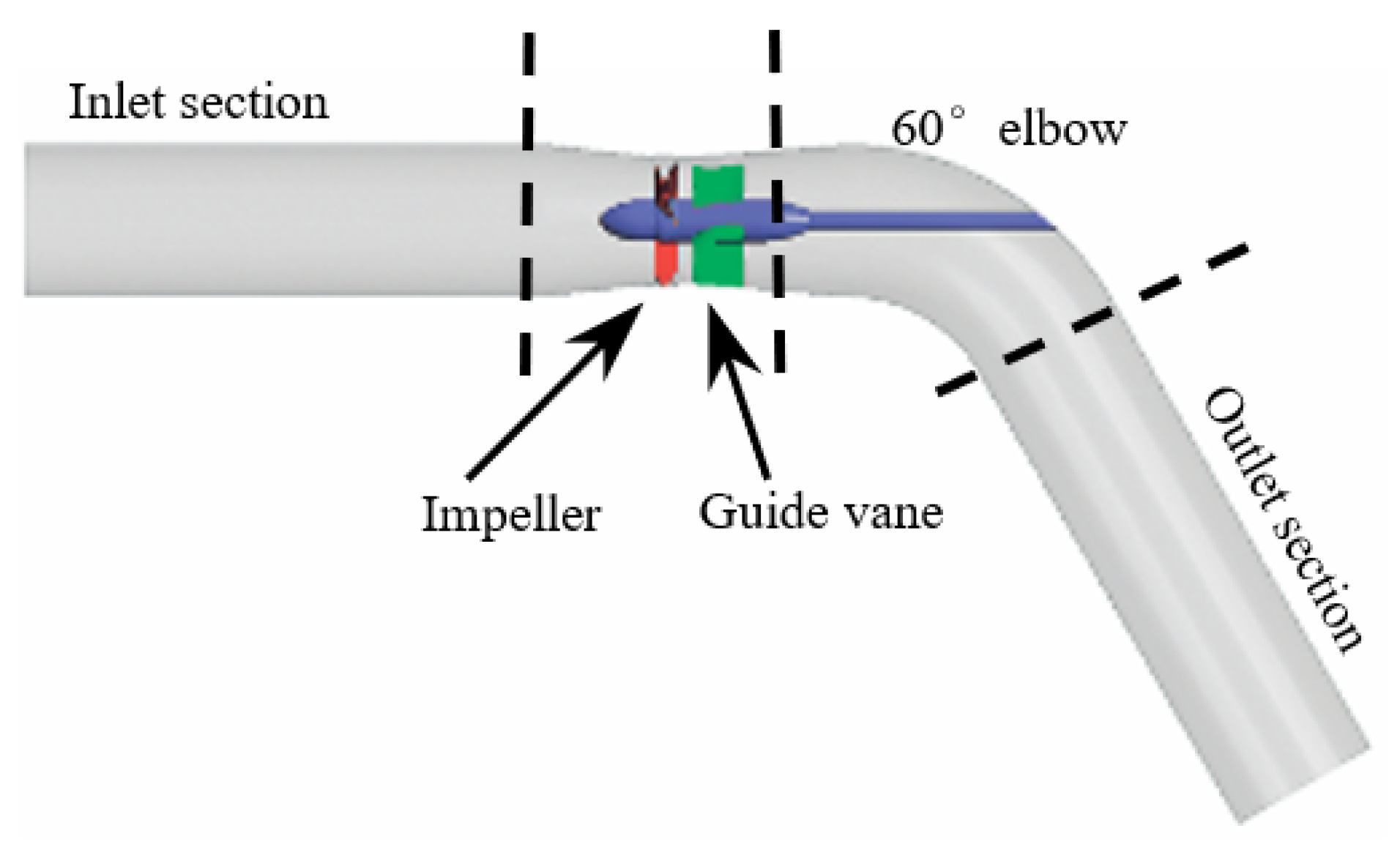
2. Research Object
3. Numerical Calculation Method
3.1. Turbulence Model and Boundary Conditions
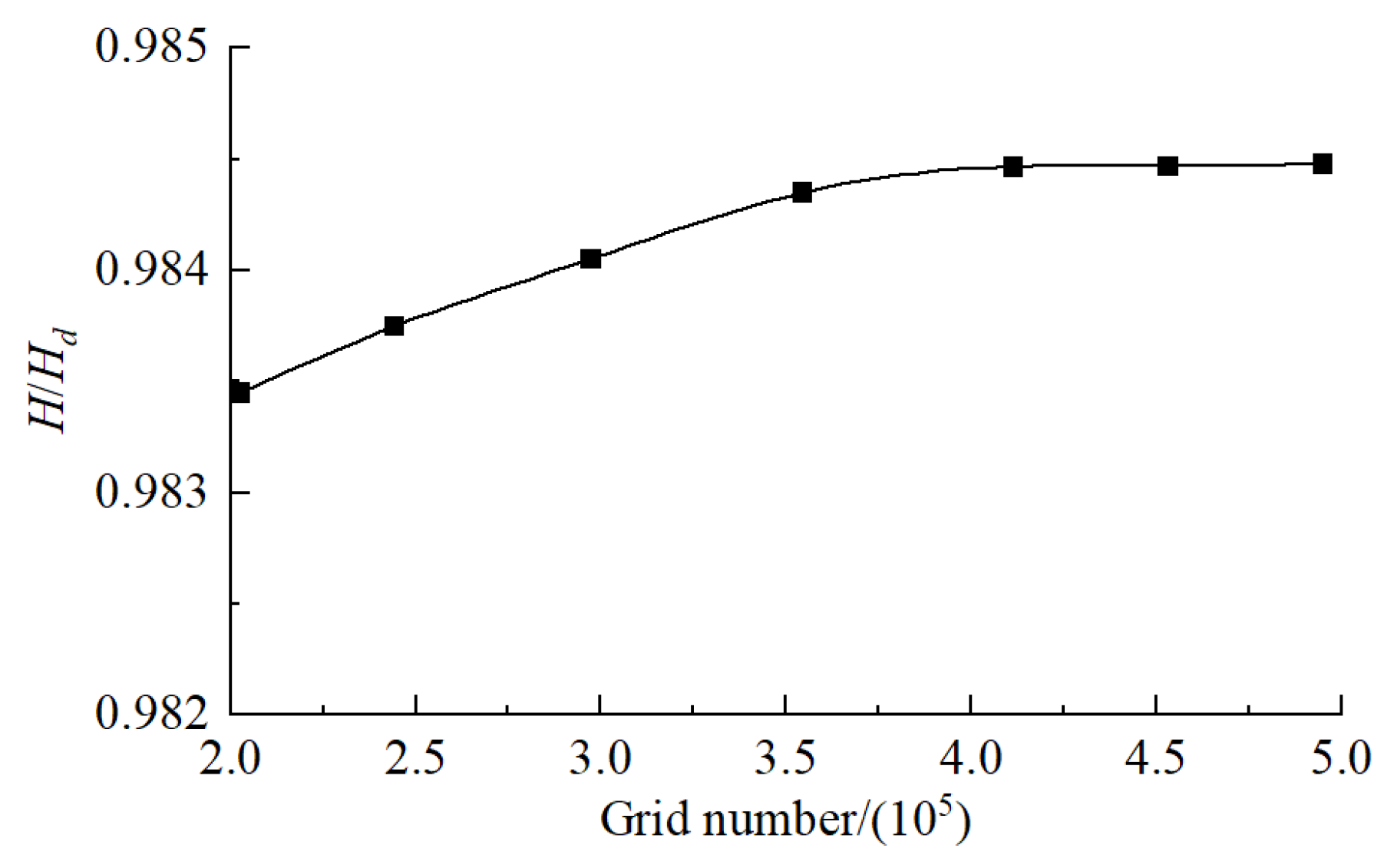
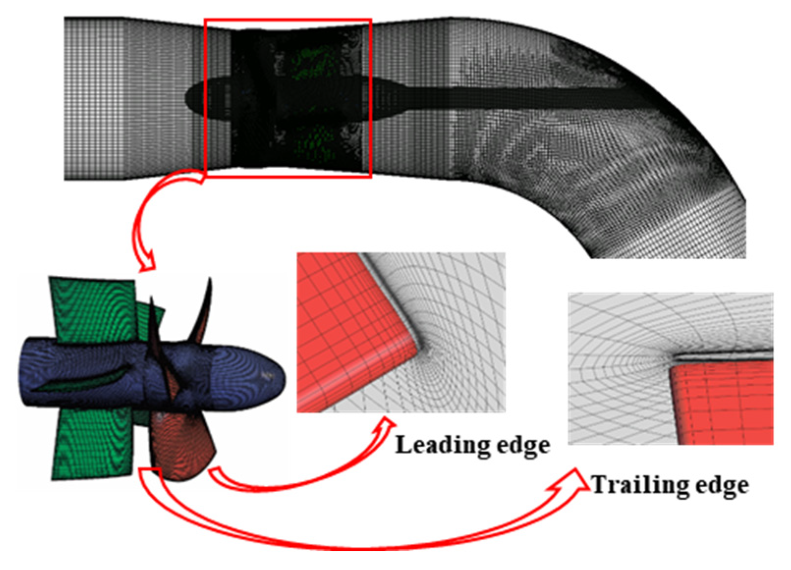
3.2. Meshing and Irrelevance Analysis
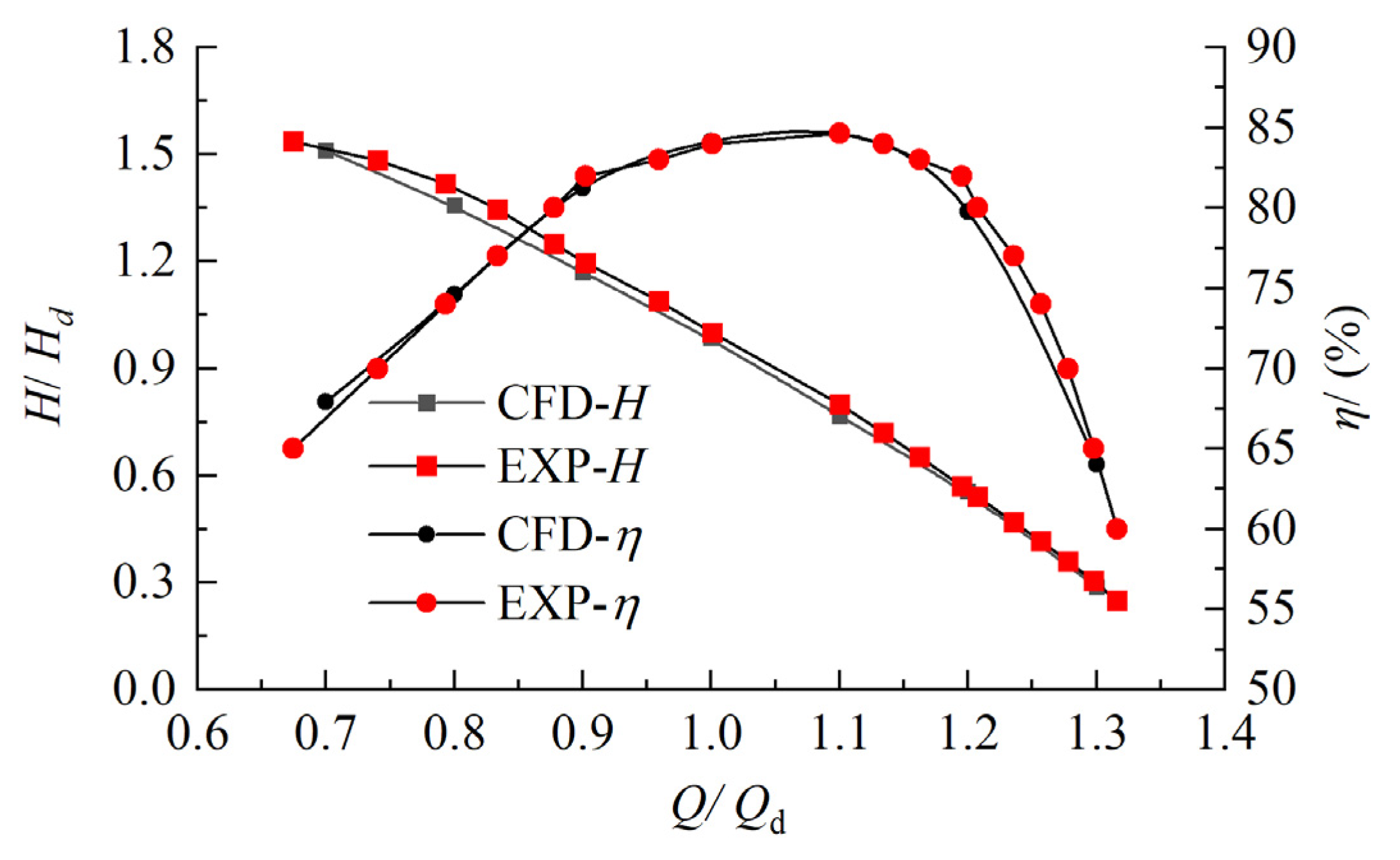
3.3. Verification of Numerical Calculation Results
4. Machine Learning Models
4.1. Support Vector Machine Regression
4.2. Gaussian Process Regression
4.3. Fully Connected Neural Network
4.4. Data Standardization and Evaluation Indicators
4.5. Hyperparameter Optimization
5. Optimization Method of Impeller
5.1. Optimization Objective
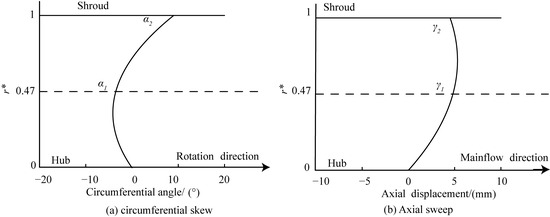
5.2. Optimization Parameters
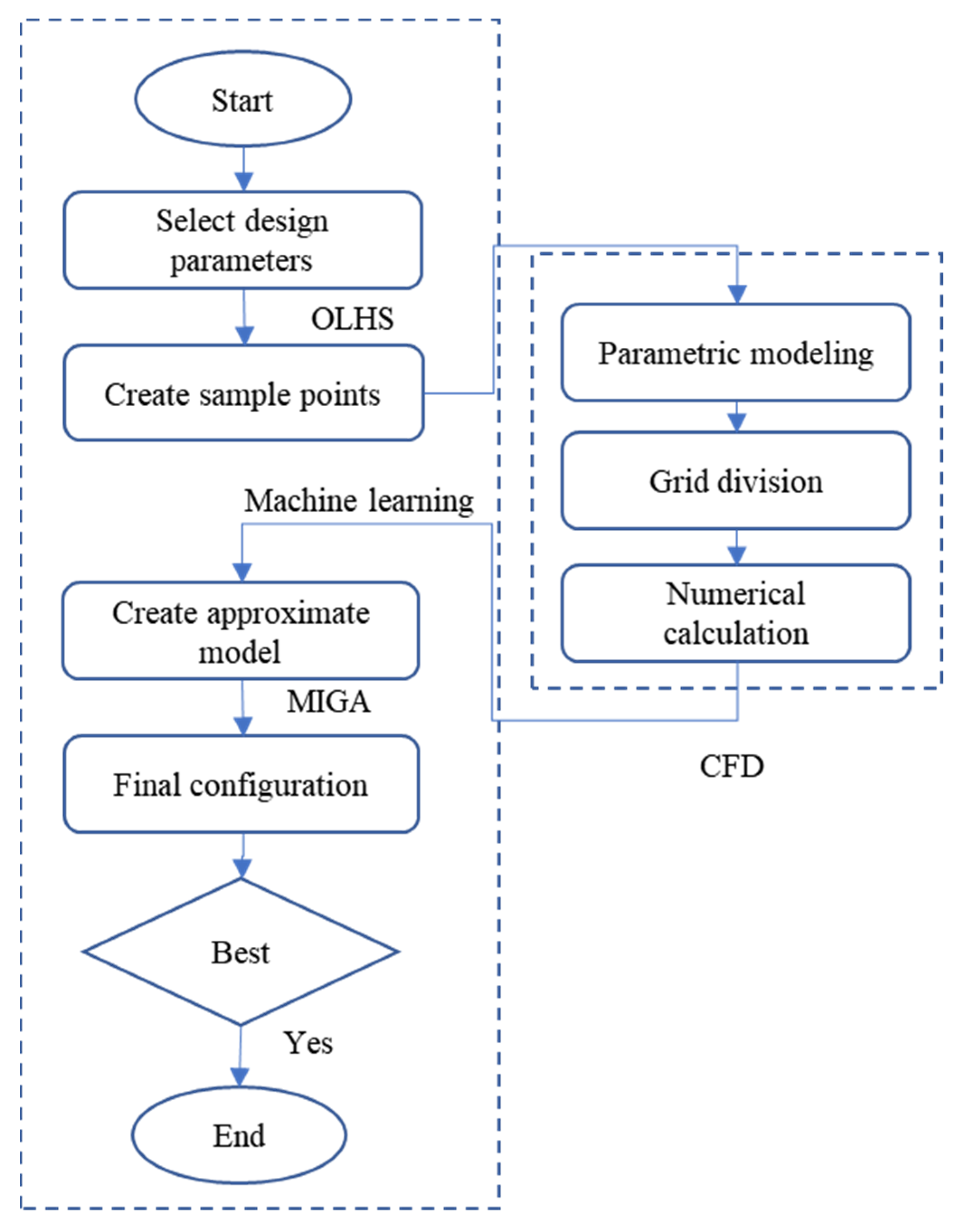
5.3. Optimization Progress
6. Results & Analysis
6.1. Data Set Partitioning
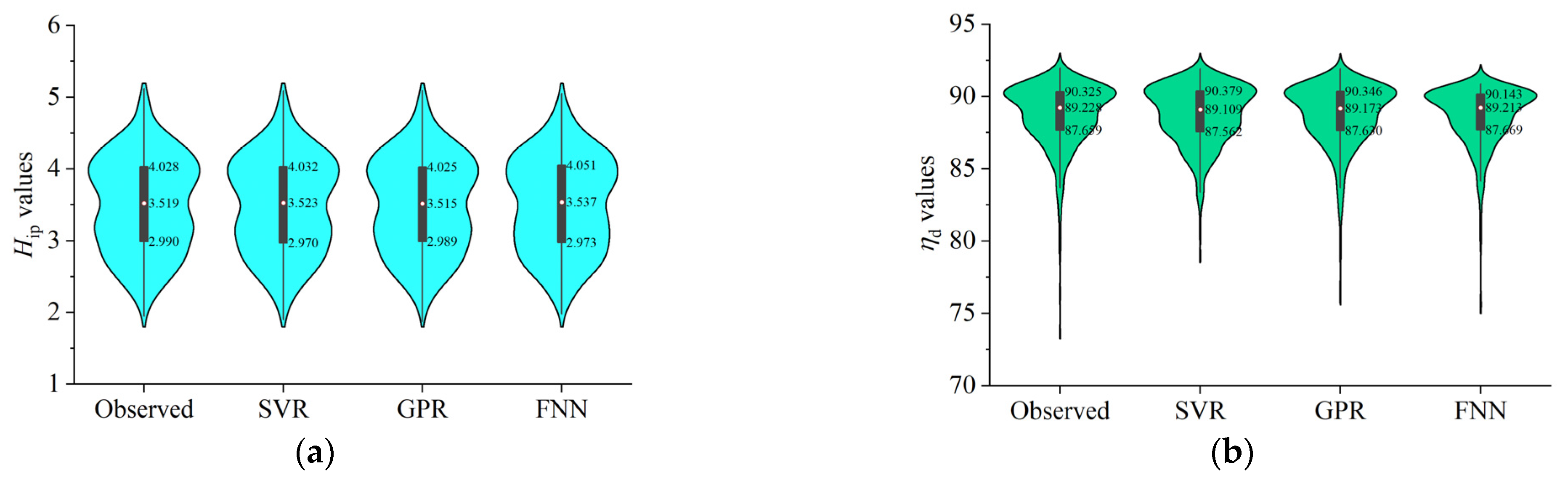
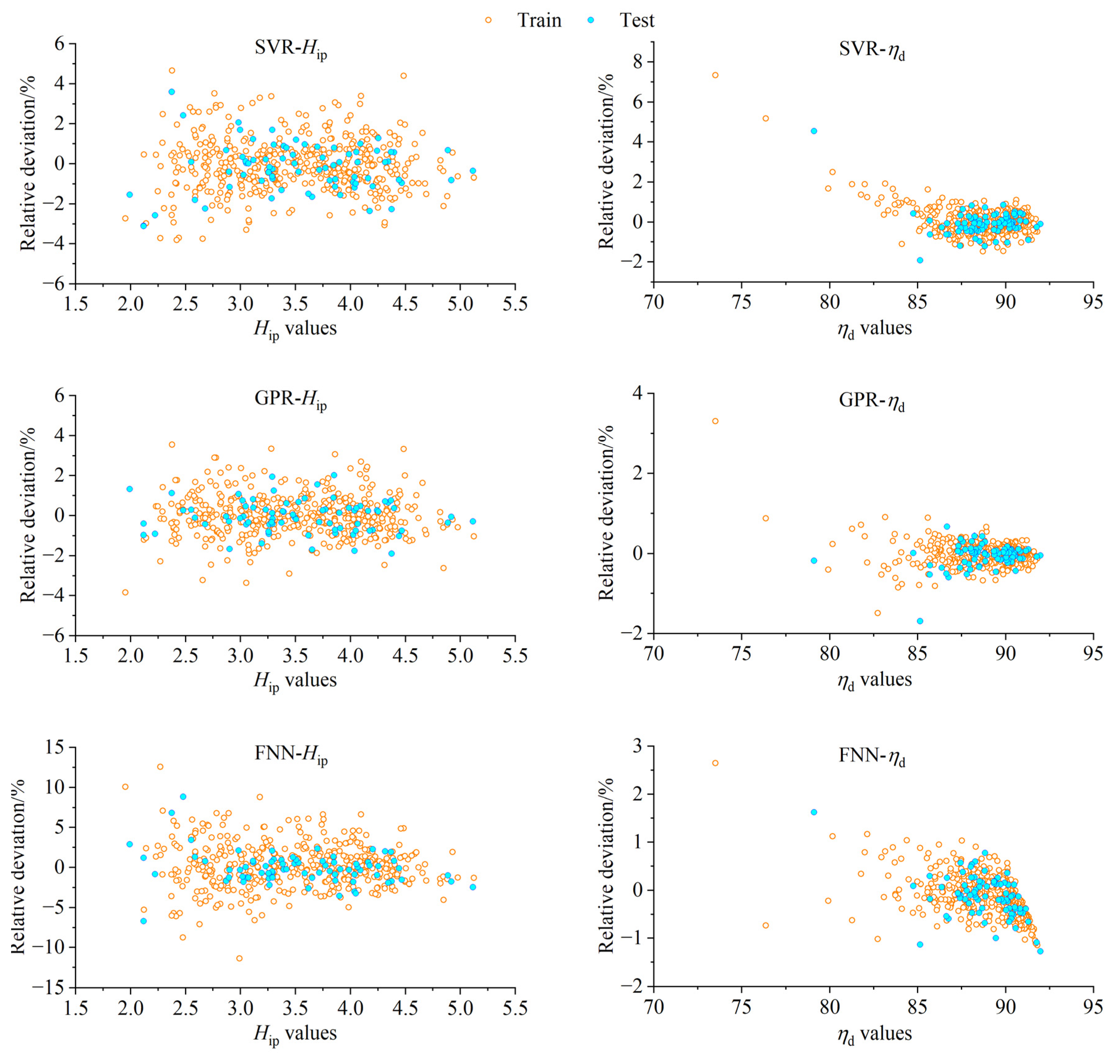
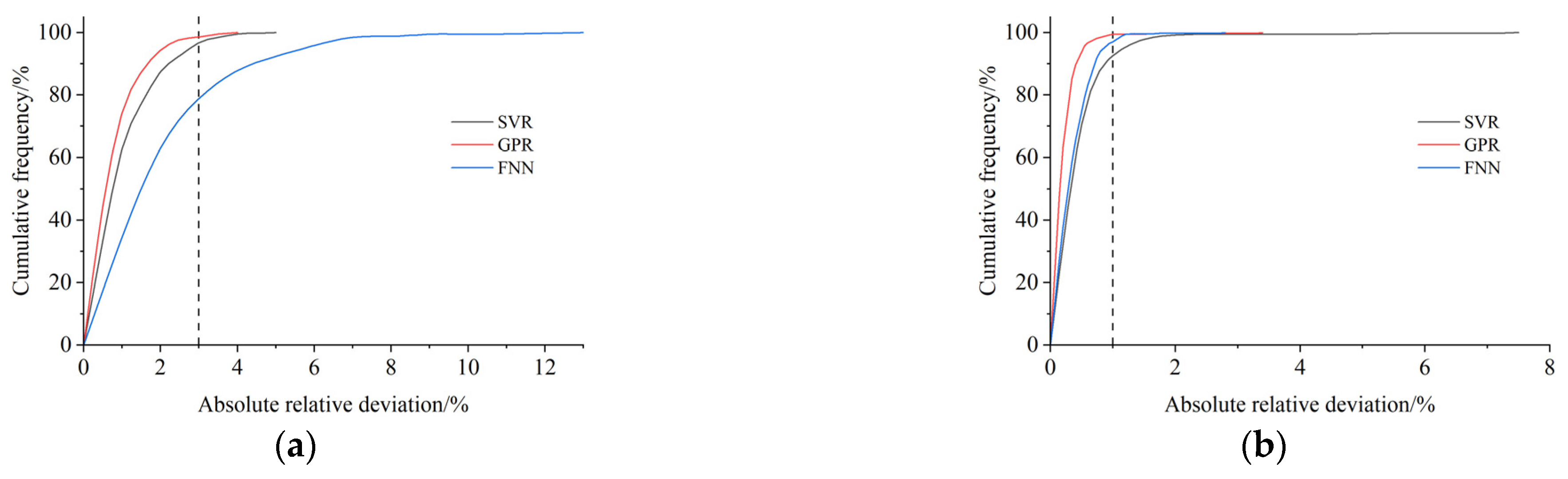
6.2. Comparison of Training Results
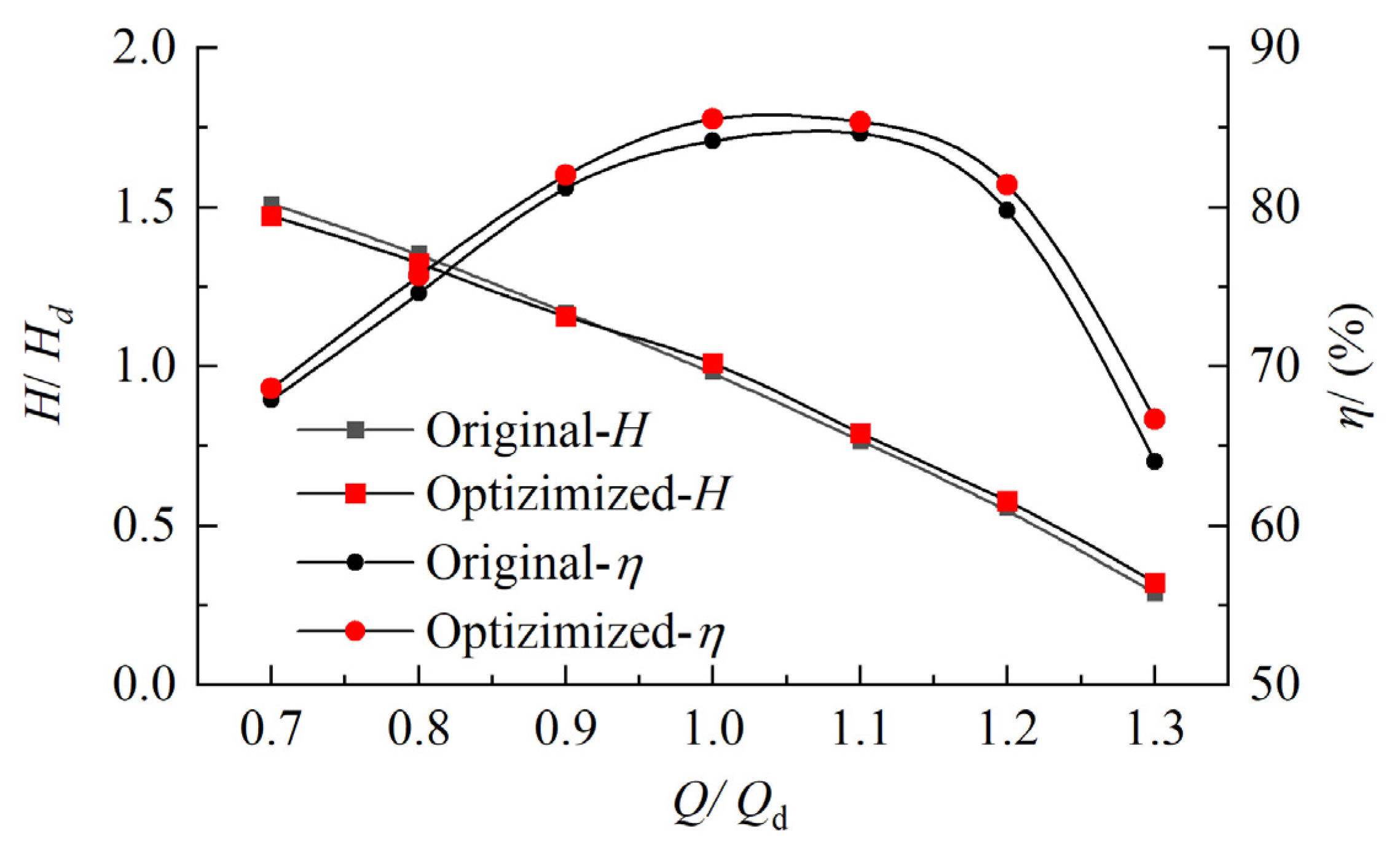
6.3. Analysis of Optimization Results
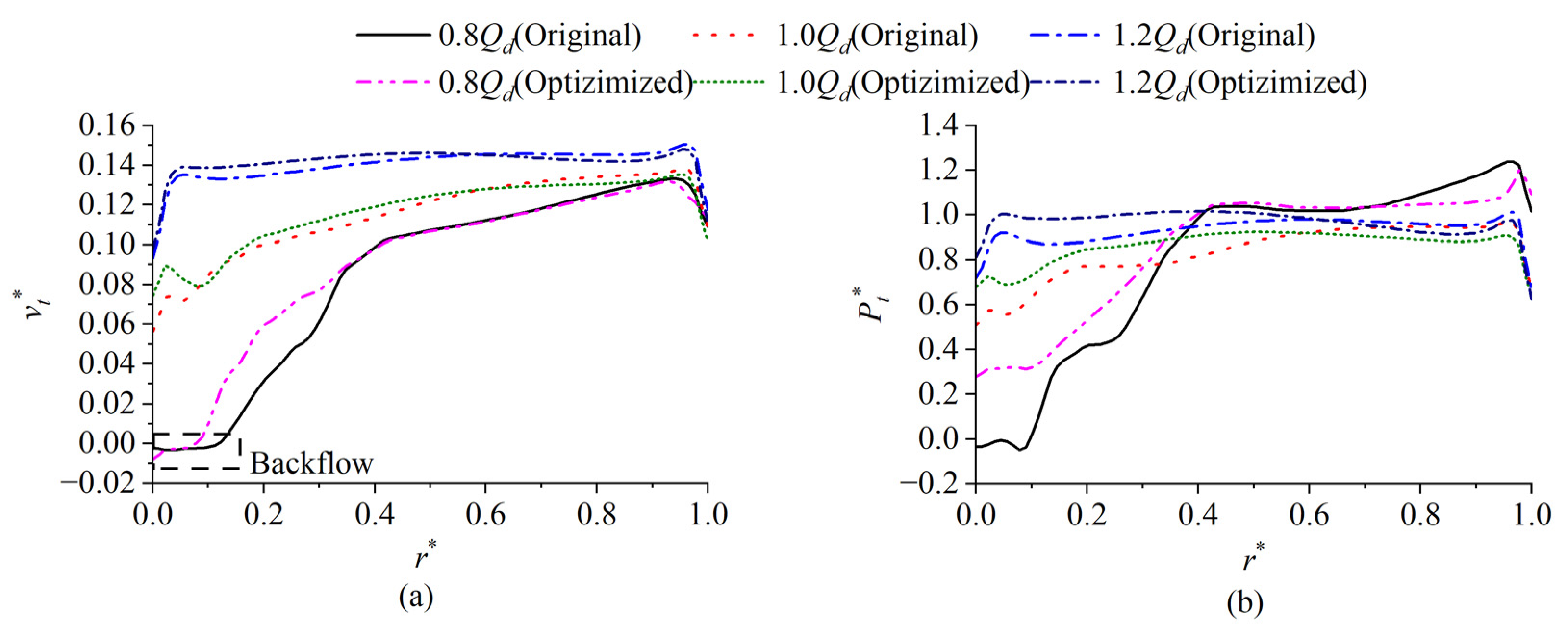
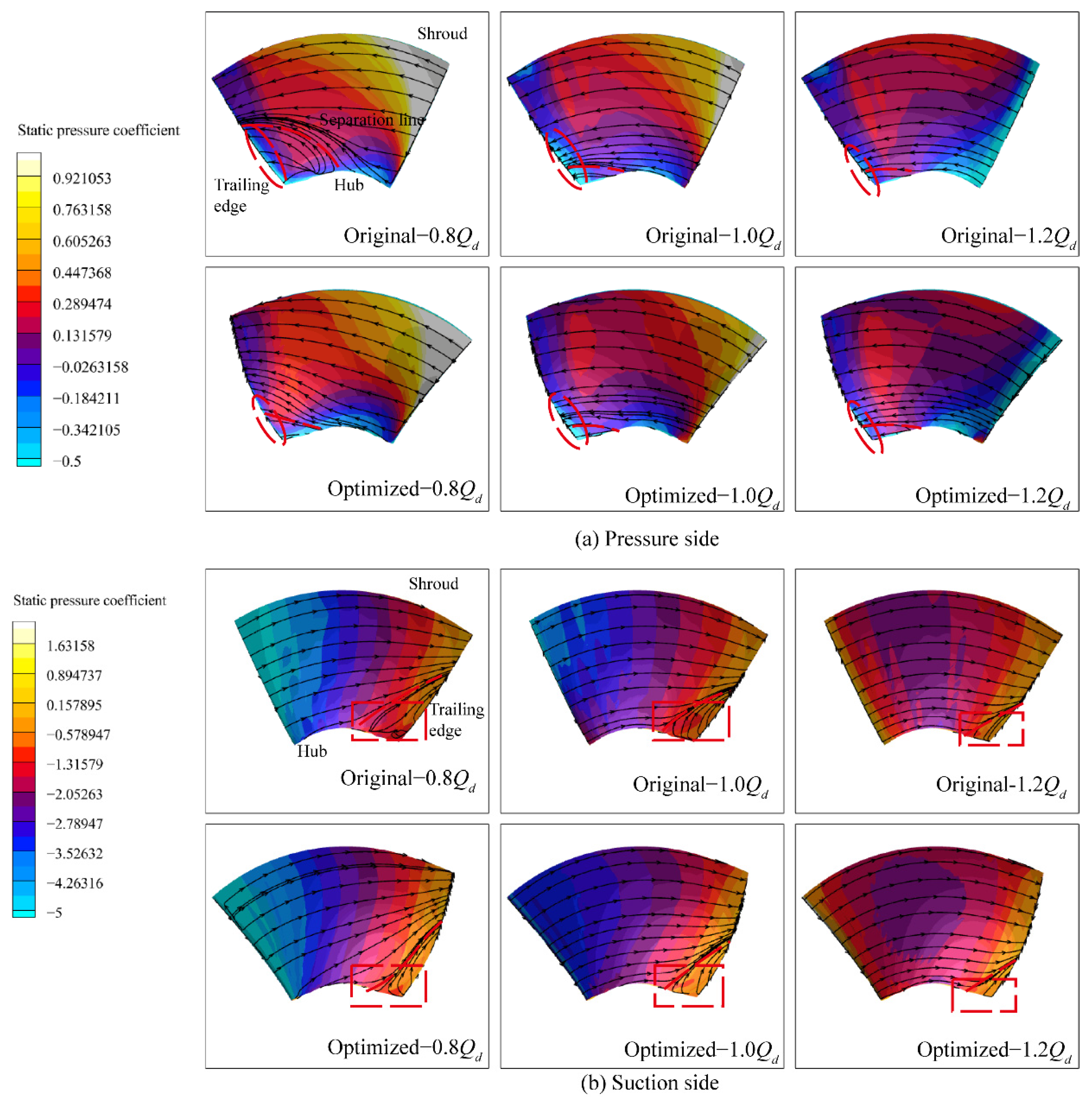
6.4. Analysis of the Internal Flow Field of the Impeller before and after Optimization
7. Conclusions
- An optimization system composed of the CFD, OLHS, ML, and MIGA is proposed, which provides a reference for the optimal design of axial flow pumps in the future.
- Based on Bayesian optimization, the hyperparameters of the SVR, FNN, and GPR models are optimized, and the optimized hyperparameter combination is used to establish the prediction model of the weighted efficiency and the impeller head. Compared to the SVR and FNN models, the GPR model has better generalization and the highest prediction accuracy, and the GPR model is better adaptable to the nonlinear relationship between the fit optimization parameters and the target in the optimal design.
- Compared to the original model, the weighted efficiency of the optimized impeller increases by 1.31 percentage points, and the efficiency of the pump section at 0.8Qd, 1.0Qd, and 1.2Qd increases by about 1.1, 1.4, and 1.6 percentage points, respectively. The operating range of the high-efficiency area of the axial flow pump is improved.
- The optimized impeller is forward skewed and backward swept, which is beneficial for reducing flow separation on the blade surface. After optimization, the flow field at the impeller outlet significantly improves; the total pressure and the axial velocity along the spanwise direction are more uniform; the flow separation at the trailing edge of the blade improves; and the entropy production in the impeller reduces.
Author Contributions
Funding
Institutional Review Board Statement
Informed Consent Statement
Data Availability Statement
Acknowledgments
Conflicts of Interest
References
- Liu, C. Researches and Developments of Axial-flow Pump System. Trans. Chin. Soc. Agric. Mach. 2015, 46, 11. [Google Scholar]
- Wang, Z.; Peng, G.; Zhou, L.; Hu, D. Hydraulic performance of a large slanted axial-flow pump. Eng. Comput. 2010, 27, 243–256. [Google Scholar] [CrossRef]
- Yang, J.; Guan, X. Hydraulic Design of High Specific Speed Model Axial-flow Pump. Trans. Chin. Soc. Agric. Mach. 2008, 39, 4. [Google Scholar]
- Shi, W. Design of Axial Flow Pump Hydraulic Model ZM931 On High Specific Speed. Trans. Chin. Soc. Agric. Mach. 1998, 29, 49–53. [Google Scholar]
- Tang, F.; Wang, G.; Liu, C.; Zhou, J.; Cheng, L. Design and Numerical Analysis On An Axial-flow Pump With High Specific Speed. J. Mech. Eng. 2005, 41, 5. [Google Scholar] [CrossRef]
- Yuan, J.; Fan, M. Orthogonal optimum design method for high specific-speed axial-flow pumps. Trans. Chin. Soc. Agric. Eng. 2018, 37, 22. [Google Scholar]
- Tao, R.; Xiao, R.; Yang, W. Optimization design for axial flow pump based on genetic algorithm. J. Drain. Irrig. Mach. Eng. 2018, 36, 7. [Google Scholar]
- Wang, L.; Wang, T.; Luo, Y. Improved NSGA- in Multi-Objective Optimization Studies of Wind Turbine Blades. Appl. Math. Mech. 2011, 32, 739–748. [Google Scholar] [CrossRef]
- Mu, X.; Yao, W.; Yu, X.; Liu, K.; Xue, F. A survey of surrogate models used in MDO. Chin. J. Comput. Mech. 2005, 22, 5. [Google Scholar]
- Gu, H.; Lin, Y.; Hu, Z.; Yu, J. Surrogate Models Based Optimization Methods for the Design of Underwater Glider Wing. J. Mech. Eng. 2009, 45, 8. [Google Scholar] [CrossRef]
- Ma, S.B.; Kim, S.; Kim, J.H. Optimization design of a two-vane pump for wastewater treatment using machine-learning-based surrogate modeling. Processes 2020, 8, 1170. [Google Scholar] [CrossRef]
- Zhu, G.; Feng, J.; Guo, P.; Luo, X. Optimization of hydrofoil for marine current turbine based on radial basis function neural network and genetic algorithm. Trans. Chin. Soc. Agric. Eng. 2014, 30, 9. [Google Scholar]
- Wang, M.; Li, Y.; Yuan, J.; Yuan, S. Effects of different vortex designs on optimization results of mixed-flow pump. Eng. Appl. Comput. Fluid Mech. 2022, 16, 36–57. [Google Scholar] [CrossRef]
- Wang, M.; Li, Y.; Yuan, J.; Meng, F.; Chen, J. Comprehensive Improvement of Mixed-Flow Pump Impeller Based on Multi-Objective Optimization. Processes 2020, 8, 905. [Google Scholar] [CrossRef]
- Wang, M.; Li, Y.; Yuan, J.; Yuan, J.; Osman, F.K. Matching Optimization of a Mixed Flow Pump Impeller and Diffuser Based on the Inverse Design Method. Processes 2021, 3, 260. [Google Scholar] [CrossRef]
- Pei, J.; Gan, X.; Wang, W.; Yuan, S.; Tang, Y. Hydraulic Optimization on Inlet Pipe of Vertical Inline Pump Based on Artificial Neural Network. Trans. Chin. Soc. Agric. Mach. 2018, 49, 8. [Google Scholar]
- Miao, S.; Yang, J.; Wang, X.; Li, J.; Li, T. Blade pattern optimization of the hydraulic turbine based on neural network and genetic algorithm. J. Aerosp. Power 2015, 30, 8. [Google Scholar]
- Feng, Y. Multi-Objective Optimum Design of Centrifugal Double-channel Pump Based on RBF Neural Network and Particle Swarm Optimization Algorithm. Ph.D. Thesis, Jiangsu University, Zhenjiang, China, 2018. [Google Scholar]
- Zhang, X.; Hu, B.; Feng, Y.; Liu, K.; Wang, C. Multi-objective optimization design of screw centrifugal pump based on RBF neural network and differential evolution algorithm. J. Drain. Irrig. Mach. Eng. 2022, 40, 7. [Google Scholar]
- Wang, C.; Ye, J.; Zeng, C.; Xia, Y.; Luo, B. Multi-objective optimum design of high specific speed mixed-flow pump based on NSGA-genetic algorithm. Trans. Chin. Soc. Agric. Eng. 2015, 31, 7. [Google Scholar]
- Wang, C.; Feng, Y.; Ye, J.; Luo, B.; Liu, K. Multi-objective parameters optimization of centrifugal slurry pump based on RBF neural network and NSGA- genetic algorithm. Trans. Chin. Soc. Agric. Eng. 2017, 33, 109–115. [Google Scholar]
- Wang, C.; Hu, B.; Feng, Y.; Liu, K. Multi-objective optimization of double vane pump based on radial basis neural network and particle swarm. Trans. Chin. Soc. Agric. Eng. 2019, 35, 25–32. [Google Scholar]
- He, D.; Li, R.; Sun, S.; Guo, P. Prediction of gas-liquid two-phase pressure increment of a centrifugal pump based on machine learning. Trans. Chin. Soc. Agric. Eng. 2022, 38, 9. [Google Scholar]
- Yang, Q.; Guo, X.; Li, Q.; Dong, W. Hot air anti-icing performance estimation method based on POD and surrogate model. Acta Aeronautica et Astronautica Sinica 2022, 44, 126992. [Google Scholar]
- Wang, W.; Yao, Y.; Ma, Z. Model of Compressor Performance Prediction Based on Error Back-propagation Artificial Neural work. Fluid Mach. 2005, 33, 4. [Google Scholar]
- Huang, R.; Zhang, Z.; Zhang, W.; Mou, J.; Zhou, P.; Wang, Y. Energy performance prediction of the centrifugal pumps by using a hybrid neural network. Energy 2020, 213, 119005. [Google Scholar] [CrossRef]
- Li, S.; Zhao, F.; Zheng, X.; He, D.; Bai, B. Wet gas metering by cone throttle device with machine learning. Measurement 2020, 164, 108080. [Google Scholar] [CrossRef]
- Chen, J.; Chen, L.; Wang, Z. The Recognition of Hydraulic Pump Leakage State Based on Wavelet Decomposition and Deep Learning. Modul. Mach. Tool Autom. Manuf. Tech. 2021, 4, 006. [Google Scholar]
- Panda, A.; Rapur, J.; Tiwari, R. Prediction of flow blockages and impending cavitation in centrifugal pumps using Support Vector Machine (SVM) algorithms based on vibration measurements. Measurement 2018, 130, 44–56. [Google Scholar] [CrossRef]
- Bordoloi, D.J.; Tiwari, R. Identification of suction flow blockages and casing cavitations in centrifugal pumps by optimal support vector machine techniques. J. Braz. Soc. Mech. Sci. Eng. 2017, 39, 2957–2968. [Google Scholar] [CrossRef]
- Rapur, S.; Tiwari, R. Severity Assessment and Classification of Blockage of Centrifugal Pumps in Frequency Domain of Vibration Data Using Support Vector Machine Algorithms. In Proceedings of the Vibrations in Rotating Machinery (VIRM-11), Manchester, UK, 13–15 September 2016. [Google Scholar]
- Zhang, S.; Tian, S.; Zhang, X.; Li, H.; Xi, D.; He, W.; Zhang, A. Research Progress of Skew and Sweep Aerodynamic Technology for Turbomachinery Blades. J. Propuls. Technol. 2021, 42, 15. [Google Scholar]
- Mao, M.; Song, Y.; Wang, Z. Research on Design of Swept and Bowed Rotor in a Transonic Axial Flow Compressor. J. Power Eng. 2008, 28, 6. [Google Scholar]
- Wei, B.; Wu, K. Review on the Research of high performance Skew-Swept Blades and Its Influence on Inner Flow. Fluid Mach. 2001, 29, 31–34. [Google Scholar]
- Li, Y.; Ouyang, H.; Du, Z. Optimized Design Based on Skewed and Swept Blade Technology. J. Eng. Therm. Energy Power 2007, 22, 605–609. [Google Scholar]
- Menter, F.; Kuntz, M.; Langtry, R. Ten years of industrial experience with the SST turbulence model. Heat Mass Transf. 2003, 4, 625–632. [Google Scholar]
- Florianr, M. Zonal two equation kw turbulence models for aerodynamic flows. In Proceedings of the 23rd Fluid Dynamics, Plasmadynamics and Lasers Conference, Orlando, FL, USA, 6–9 July 1993; p. 2906. [Google Scholar]
- Lee, K.S.; Ziaul, H.; Han, S.E. A study on the y+ effects on turbulence model of unstructured grid for CFD analysis of wind turbine. J. Korean Assoc. Spat. Struct. 2015, 15, 75–84. [Google Scholar] [CrossRef] [Green Version]
- Zhou, Z.H. Machine Learning; Springer Nature: Berlin/Heidelberg, Germany, 2021. [Google Scholar]
- Vapnik, V.; Golowich, S.; Smola, A. Support Vector Method for Function Approximation, Regression Estimation and Signal Processing. Adv. Neural Inf. Process. Syst. 1996, 9, 281–287. [Google Scholar]
- Rasmussen, C.E.; Williams, C.K.I. Gaussian Processes for Machine Learning; The MIT Press: Cambridge, MA, USA, 2006. [Google Scholar]
- Hsu, K.Y.; Li, H.Y.; Psaltis, D. Holographic implementation of a fully connected neural network. Proc. IEEE 1990, 78, 1637–1645. [Google Scholar] [CrossRef] [Green Version]
- Gourisaria, M.K.; Mishra, B.; Dehuri, S. A Hybrid Parallel Multi-Objective Genetic Algorithm: HybJacIsCone Model. Int. J. Comput. Appl. 2013, 66, 1–6. [Google Scholar]
- Sun, L.; Pan, Q.; Zhang, D.; Zhao, R.; van Esch, B. Numerical study of the energy loss in the bulb tubular pump system focusing on the off-design conditions based on combined energy analysis methods. Energy 2022, 258, 124794. [Google Scholar] [CrossRef]
- Ji, L.; Li, W.; Shi, W.; Chang, H.; Yang, Z. Energy characteristics of mixed-flow pump under different tip clearances based on entropy production analysis. Energy 2020, 199, 117447. [Google Scholar] [CrossRef]


| Model | Hyperparameter and Its Search Range |
|---|---|
| SVR | Kernel functions: Gaussian, linear, cubic, and quadratic Regularization factor: [0.001,1000] Kernel scale: [0.001,1000] ε: [0.001,100]/1.349·iqr(Y) |
| GPR | Basis functions: zero, constant, and linear. Kernel functions: Non-isotropic and isotropic exponential, quadratic rational, squared exponential, Matern 5/2, and Matern 3/2 Kernel scale: [0.001, 1] ·(max(X)–min(X)) Standard Deviation: [0.0001, max (0.001, 10×std(Y))] |
| FNN | Number of fully connected layers: [1,2,3] Size of each connection layer: [1,300] Activation function: Rectified Linear Unit (RELU), Tanh, None, and Sigmoid Regularization strength: [0,1250] |
| Design Parameters | Low Level (−) | High Level (+) |
|---|---|---|
| (c/t)1/- | 0.679 | 0.829 |
| (c/t)2/- | 0.522 | 0.638 |
| β1/° | 39.435 | 48.199 |
| β2/° | 24.816 | 30.330 |
| β3/° | 15.817 | 19.331 |
| (a/c)1/% | 5.470 | 6.686 |
| (a/c)2/% | 3.154 | 3.854 |
| (a/c)3/% | 1.362 | 1.664 |
| γ1/mm | −5 | 10 |
| γ2/mm | −5 | 10 |
| α1/° | −15 | 15 |
| α2/° | −15 | 15 |
| Data Set | Sample Size | Max Value | Min Value | Mean Value | Standard Deviation | |
|---|---|---|---|---|---|---|
| Hip2 | Training set | 439 | 5.123 | 1.952 | 3.494 | 0.660 |
| Testing set | 77 | 5.114 | 1.993 | 3.540 | 0.669 | |
| ηd | Training set | 439 | 91.796 | 73.497 | 88.707 | 2.281 |
| Testing set | 77 | 91.972 | 79.107 | 88.795 | 1.904 | |
| Evaluation Indicators | SVR | GPR | FNN | ||||
|---|---|---|---|---|---|---|---|
| Training Set | Testing Set | Training Set | Testing Set | Training Set | Testing Set | ||
| Hip2 | R2 | 0.995 | 0.997 | 0.997 | 0.998 | 0.982 | 0.991 |
| MSE | 0.002 | 0.001 | 0.001 | 0.001 | 0.008 | 0.004 | |
| MAPE | 1.016 | 0.945 | 0.772 | 0.634 | 2.082 | 1.416 | |
| RAE | 0.061 | 0.058 | 0.047 | 0.041 | 0.122 | 0.087 | |
| WIA | 0.999 | 0.999 | 0.999 | 1.000 | 0.995 | 0.998 | |
| ηd | R2 | 0.937 | 0.898 | 0.988 | 0.986 | 0.971 | 0.954 |
| MSE | 0.324 | 0.364 | 0.063 | 0.070 | 0.150 | 0.166 | |
| MAPE | 0.440 | 0.429 | 0.198 | 0.195 | 0.346 | 0.348 | |
| RAE | 0.224 | 0.270 | 0.101 | 0.124 | 0.179 | 0.222 | |
| WIA | 0.984 | 0.975 | 0.997 | 0.995 | 0.993 | 0.988 | |
| Design Parameters | Original | Optimized |
|---|---|---|
| (c/t)1/- | 0.754 | 0.819 |
| (c/t)2/- | 0.580 | 0.594 |
| β1/° | 43.817 | 47.792 |
| β2/° | 27.573 | 28.106 |
| β3/° | 17.574 | 16.847 |
| (a/c)1/% | 6.078 | 5.571 |
| (a/c)2/% | 3.503 | 3.845 |
| (a/c)3/% | 1.513 | 1.655 |
| γ1/mm | 0 | 6.531 |
| γ2/mm | 0 | 6.981 |
| α1/° | 0 | −3.93 |
| α2/° | 0 | −7.98 |
| ηd/% | 90.91 | 92.22 |
| Hip/m | 3.660 | 3.699 |
Publisher’s Note: MDPI stays neutral with regard to jurisdictional claims in published maps and institutional affiliations. |
© 2022 by the authors. Licensee MDPI, Basel, Switzerland. This article is an open access article distributed under the terms and conditions of the Creative Commons Attribution (CC BY) license (https://creativecommons.org/licenses/by/4.0/).
Share and Cite
Sun, Z.; Tang, F.; Shi, L.; Liu, H. Multi-Conditional Optimization of a High-Specific-Speed Axial Flow Pump Impeller Based on Machine Learning. Machines 2022, 10, 1037. https://doi.org/10.3390/machines10111037
Sun Z, Tang F, Shi L, Liu H. Multi-Conditional Optimization of a High-Specific-Speed Axial Flow Pump Impeller Based on Machine Learning. Machines. 2022; 10(11):1037. https://doi.org/10.3390/machines10111037
Chicago/Turabian StyleSun, Zhuangzhuang, Fangping Tang, Lijian Shi, and Haiyu Liu. 2022. "Multi-Conditional Optimization of a High-Specific-Speed Axial Flow Pump Impeller Based on Machine Learning" Machines 10, no. 11: 1037. https://doi.org/10.3390/machines10111037