Piecewise Decoupling Tool Orientation Re-Scheduling for Four-Axis Reciprocal Toolpaths of Blades Based on S-θ Plane with Monotonicity Constraint

Abstract

Reciprocal toolpaths with four-axis simultaneous motion of five-axis or four-axis machine tools are commonly used in the machining of blades which are widely applied in high-end equipment such as the aero-engine and the marine steam turbine. Due to the complex geometry of the blades, the tool orientation always suffers from frequent swing for this kind of toolpaths, which induces unnecessary acceleration/deceleration of the feed axes, thus degrading processing efficiency and quality. Although there are tool orientation optimization methods aiming at solving the above problem, they are mainly proposed for universal processing of the toolpaths for complex surfaces. Different from them, this paper proposes a piecewise decoupling tool orientation re-scheduling method for this kind of toolpath specifically, which takes full use of the characteristic of the reciprocal toolpaths of the blades, and takes the monotonous variation of rotation axes as an additional constraint. The re-scheduling process is realized based on the construction of a $S$-$\theta$ plane, where the scheduling problem is converted to the adjustment of a $S$-$\theta$ curve inside a feasible channel. Through two procedures, namely linearization scheduling and control-point assigning-based smoothing, the tool orientation path expressed by the $S$-$\theta$ curve can be effectively scheduled in a piecewise manner, and the smoothness between two adjacent pieces of the toolpaths can be ensured directly. The whole algorithm is lightweight and does not involve complex iterative operations or functional optimization solutions. Simulation and experimental tests verify the feasibility and superiority of this method. The results show that the machining efficiency of the blade is improved by 24.5%, due to the reduction of the requirement on highest feed-axis kinematics parameters after rescheduling. In addition, compared with the existing methods, the proposed method not only can improve the dynamics of feed axes in multi-axis machining, but also has advantages in computational complexity and monotonic variation property of the tool orientation.

1. Introduction

Blades are key parts of many high-end equipment such as the aero-engine and the marine steam turbine, therefore, they play important roles in aerospace, marine, and automotive fields. Due to the complex geometric shape of the blades, four-axis or five-axis NC machining has become the mainstream way for the machining of blades [1]. For the positions away from the blade root and the blade crown, they are mainly machined by five-axis simultaneous motion using torus cutters, thus realizing high-efficiency wide-line cutting, while for the positions near the blade root or the blade crown where the interference appears easily, they are mainly machined by four-axis simultaneous motion with a fixed fifth rotary axis, using ball-end cutters, thus avoiding interference with the root or crown. Since there are many generalized five-axis toolpath optimization methods, this paper focuses on the four-axis toolpath optimization of the blades specifically [2].

At present, most multi-axis NC machining methods take CAM software to directly generate toolpaths with fixed rake and roll angles; however, due to the characteristics of sharp and frequent variation on curvature and concavity-convexity, this will lead to sharp direction variation and frequent swing of the scheduled tool orientation, which further result in sharp fluctuation in the velocity of the rotary and translational axes of the machine tool, thus ultimately decreasing the processing efficiency and quality [3].

In order to solve the above problems, it is necessary to reschedule and optimize the tool orientation. At present, the existing optimization methods of tool orientation in NC machining are mainly carried out from two aspects: to realize the global interference avoidance in geometry and the smooth variation of tool orientation in the feasible region.

Many effective methods have been proposed to construct the feasible region of tool orientation without global interference. Jun et al. [4] proposed the construction method of the feasible region of tool orientation in the $\alpha$-$\beta$ plane, which can meet the requirements of residual height and the constraints of machining interference. Lin et al. [5] proposed a collision avoidance method by judging whether the selected surface points were inside the space of cutter. Wang et al. [6] proposed the graphics-assisted collision avoidance method by identifying the contribution of pixels on the circular area of colorful collision map. By tessellating workpiece and machine tools into polygons, Ilushin et al. [7] presented the polygon/surface–tool intersection algorithm to detect the global collision in multi-axis machining. By representing the workpiece surface as point clouds, Ho et al. [8] realized the real-time collision avoidance based on the bounding box hierarchy method. Choi et al. [9] tried to complete the generation strategy of toolpath in C-space, which is a feasible region of tool orientation constructed with no overcut, no undercut, and no global interference and collision as constraints. Lu et al. [10] proposed a three-dimensional configuration space (3D C-space) method by introducing cutter lift height along normal of workpiece surface as the third variable. Mi et al. [11] simplified the C-space method by only identifying the boundary of collision-free area. Balasubramaniam et al. [12,13] proposed a visibility map (Vmap) method using the concept of visibility to generate a global collision-free tool orientation feasible region. To extend the application of Vmap, Wang and Tang [14] proposed a feasibility map (Fmap) method based on Vmap to generate the collision-free toolpath.

The above methods can indeed achieve geometric tool interference collision avoidance. However, in order to pursue the universality of feasible region construction methods, they have more or less made a compromise on the computational complexity. For the four-axis helical reciprocal machining of blades, the above methods are feasible but redundant. Therefore, it is necessary to find a simple and feasible method to construct the feasible region of tool orientation for the machining of such parts.

After obtaining the feasible region of tool orientation, the smoothness of tool orientation changes on adjacent tool contacts and even on the whole toolpath has become the primary problem of tool orientation scheduling. For the problem of how to schedule the tool orientation in the feasible region, Lauwers et al. [15] proposed a method to smooth the tool orientation by controlling the swing angle of the tool orientation on the unit path. Ho et al. [16] interpolated the vector of key points in the form of quaternion to obtain a relatively smooth tool orientation. Bi et al. [17] established a collision-free toolpath generation scheme based on a GPU-based (graphics process unit) algorithm. Sun et al. [18] proposed a double spline tool orientation smoothing method along the specified feedrate contour with the constraints of the velocity, acceleration, and jerk limit of tool swing. Farouki et al. [19] optimized the variation characteristics of the rotary axis by using the minimal rotating frame while maintaining a constant cutting velocity, thus realizing the optimization of the tool orientation smoothness. Huang et al. [20] used the radial basis function to perform fairing interpolation on the specified tool orientation at the key CC point, so as to determine the tool orientation at other CC point. Based on the algorithm of differential evolution and sequence linear programming, Lu et al. [21] realized the tool orientation smoothing of the selected path segment. Castagnetti et al. [22] establish an optimization objective function with the objective of minimizing the variation of the rotary axis, and use the gradient-based optimization method to calculate it. Hu and Tang [23] take the minimum angular acceleration of the rotation axis as the optimization objective and use the heuristic genetic algorithm to determine the optimal tool orientation. Xu et al. [24] also aimed at minimizing the angular acceleration of the rotary axis and smoothed the tool orientation utilizing least square interpolation and interference check reciprocal iteration.

It can be seen that there are many methods proposed for the smooth scheduling of tool orientation within the feasible range. With the increase of the complexity of constraints and objective function, the smoothness of tool orientation variation also becomes better. However, most existing methods mainly concern the smoothness of the variation of the tool orientation, instead of the monotonicity, and most of them have a large computation burden.

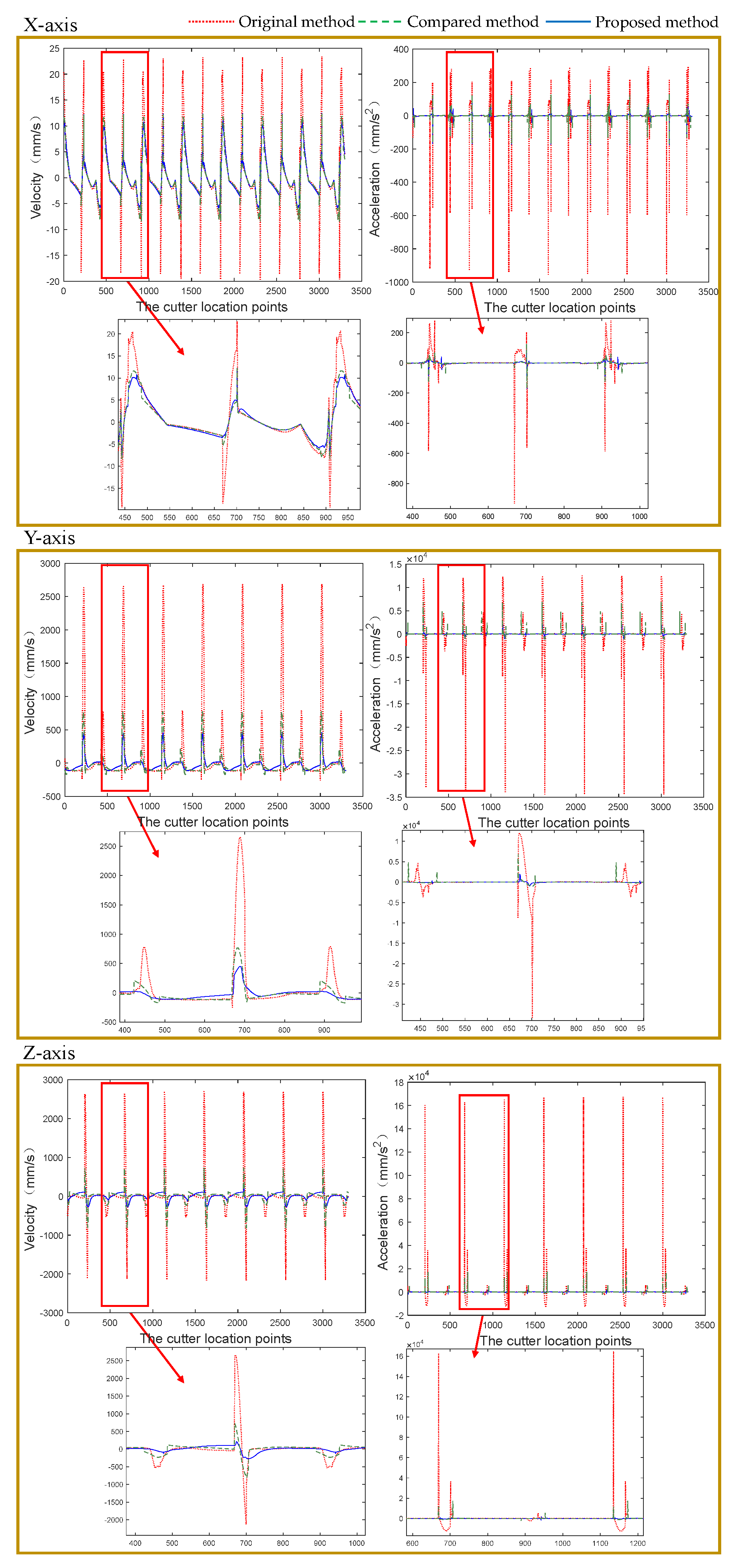
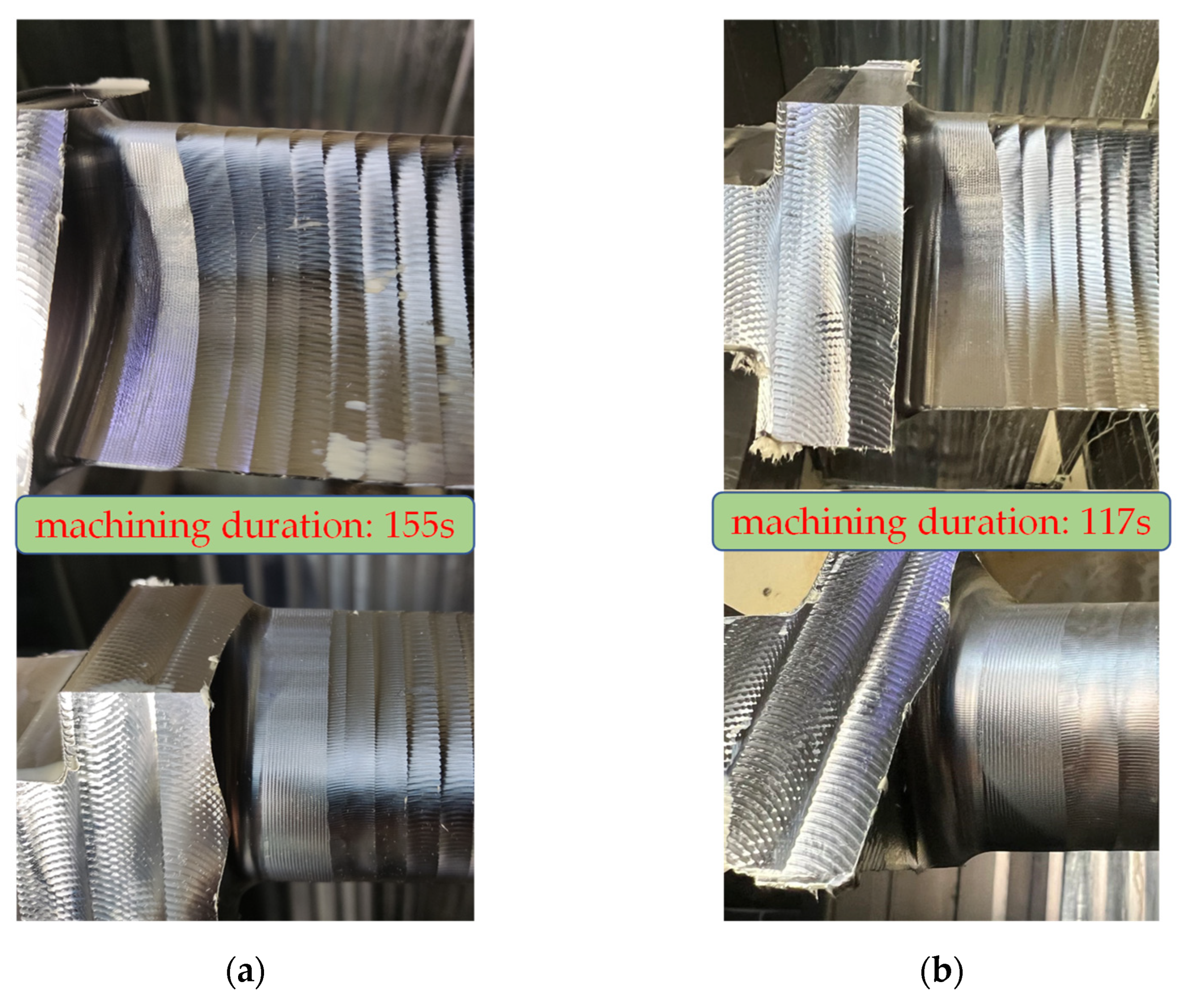
According to the cyclic characteristics of the blade-machining toolpaths, this paper proposes a piecewise decoupling tool orientation scheduling method, which realizes the monotonous variation, global high-order smoothness, and global interference-free of the re-scheduled tool orientation. This is realized by the construction and scheduling in a $S$-$\theta$ plane, where $S$ represents the motion distance of the cutter location and $\theta$ is the motion angle of the tool orientation. Through experimental verification, it is seen that this method can greatly reduce the velocity and acceleration fluctuation of not only the rotary axis but also translational axes of the machine tool, and significantly improve the processing efficiency without the sacrificing of the machining quality.

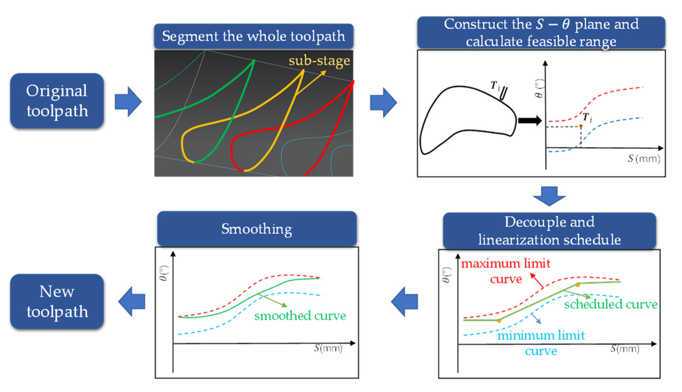
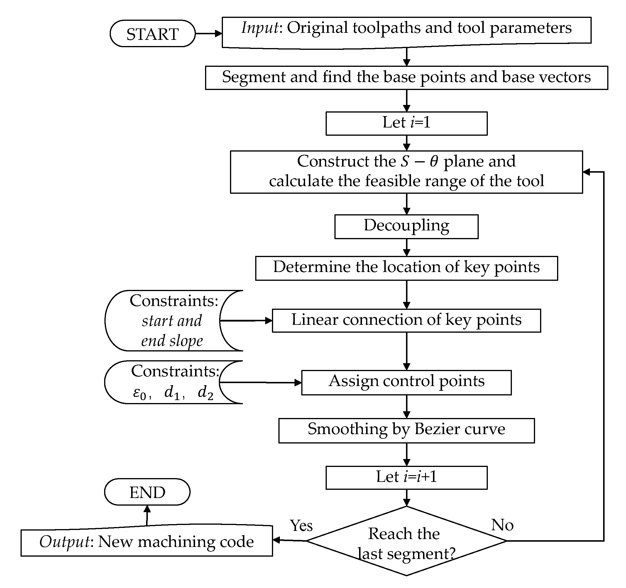
The specific steps of this method are shown in Figure 1. Firstly, the whole toolpath is segmented by taking the concave and convex variation points of the blade as nodes, and the limit tool orientation at each node is selected as the base vector. Then, the $S$-$\theta$ plane is constructed based on the base vector, and the feasible region of tool orientation is calculated in this plane. After that, aiming at the monotonic variation of the tool orientation, the segmented toolpath is decoupled, and the linearization scheduling of the tool orientation is completed by selecting the key points on the boundary of the feasible region. Finally, using Bezier curves based on the assignment of control points, the tool orientation is smoothed with the goal of minimizing the acceleration of the rotary axis, so as to obtain the tool orientation curve with G2 continuity and monotonic variation.

For the four-axis tool orientation re-scheduling of the blades, the presented method in this paper has the following two different characteristics:

(1) Most existing methods aim at global smoothness of the tool orientation. Therefore, the optimization should be conducted by taking all of the integral toolpath information into consideration simultaneously. Obviously, this strategy requires severe computational complexity, which is excessively redundant for the machining toolpaths of the blades because of the distinct reciprocal characteristic. To deal with this problem, this paper presents a piecewise tool orientation re-scheduling method, so as to release the computational burden as much as possible by taking full use of the reciprocal geometric characteristic of the blades machining toolpaths.

(2) Although existing methods yield smoothest toolpaths in theory, they may not perform ideally when applied in practice. This is because the existing methods did not take the monotonous motion of physical feed axes into consideration. However, due to the inevitable reverse clearance of the actual machine tool structure, the frequent reciprocal swing of feed axes must cause impact on the machining quality and efficiency in actual machining. To deal with this problem, this paper takes the monotonous motion of physical rotary axis as a key constraint.

In Section 2, the realization method of piecewise decoupling of tool orientation and the specific process of linearization scheduling will be introduced in detail. In Section 3, the Bezier curve smoothing method based on the assignment of control points will be introduced. In order to prove the feasibility of this method, the simulation and experimental results of this method will be shown and analyzed in Section 4. Finally, the proposed method will be summarized in Section 5.

2. Piecewise Decoupling Tool Orientation Scheduling for Reciprocal Toolpaths with a Monotonic Motion of Rotary Axis

A piecewise decoupling tool orientation linearization scheduling method is presented in this section. The proposed method can realize the monotonic variation of the tool orientation without involving complex function calculation. The main contents of this method include segmentation, the construction of the $S$-$\theta$ plane, decoupling, and linearization scheduling. Detail of the piecewise decoupling tool orientation linearization scheduling method is presented in following subsections.

2.1. Construction of the S-θ Plane and Calculation of Feasible Region of Tool Orientation

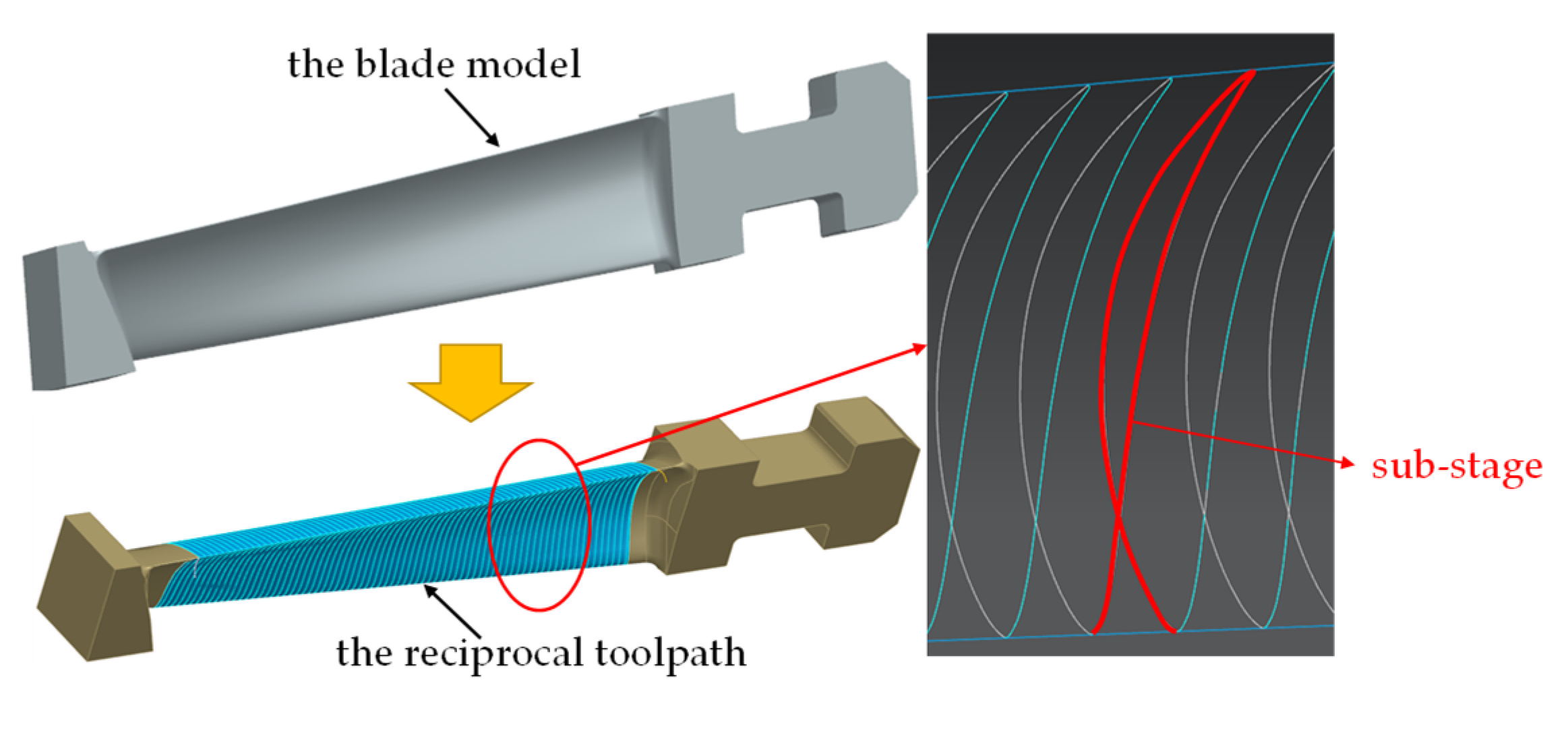
According to the helical cyclic reciprocal machining characteristics of blades, the variation of tool orientation can be divided into two parts: circular motion around the blade and linear motion in the direction of the vertical section. With the help of the idea of microelement, this method decomposes the linear motion into multiple layers, thus regarding the helical machining of the blade as the accumulation of the cross-section machining of layers. By taking the tool orientation path within one layer turning around the blade for one cycle as a sub-stage, it can be realized to complete the scheduling of the overall toolpath in a piecewise manner, as shown in Figure 2, so that the overall optimization problem can be decoupled, which releases the redundant computational complexity.

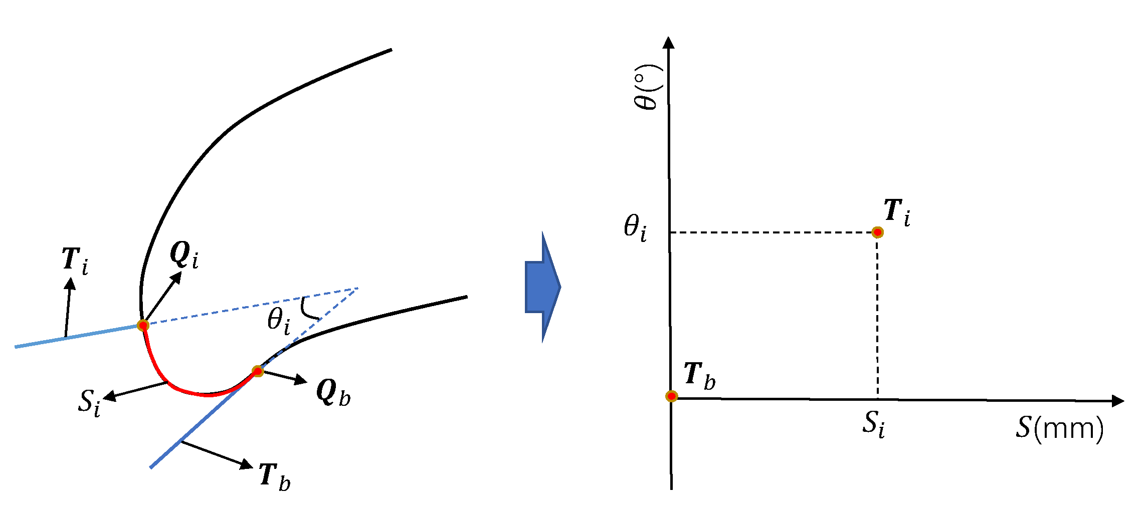
The cutter location trajectory of each sub-stage is the corresponding blade section curve, and usually, the node with special significance on the blade section curve is the concave-convex altered point on the curve. Therefore, this method selects a concave-convex altered point of the blade section curve as the base point and takes the limit tool orientation at the base point as the base vector. Take the base point as the reference for computing the arc length of other tool locations within the current layer, and the arc length is marked as $S$ here, being the abscissa parameter of the $S$-$\theta$ plane. Correspondingly, mark the rotation angle of other tool orientations relative to the base vector as $\theta$, being the ordinate parameter of the $S$-$\theta$ plane, thus the $S$-$\theta$ plane can be established. Most of the following work in this method will be carried out on the $S$-$\theta$ plane. The mapping relationship between the tool orientation in the section of blade layers and the point in $S$-$\theta$ plane is shown in Figure 3, where ${\mathit{Q}}_b$ and ${\mathit{T}}_b$ are the base point and base vector, respectively, and ${\mathit{Q}}_i$ and ${\mathit{T}}_i$ are a tool location on the section and its corresponding tool orientation, respectively.

For the calculation of the feasible range of the tool orientation, the first thing is to search the limit position of the tool under geometric constraints in the forward and backward directions at each cutter location. It should be noted that in this method, the feed direction of the tool is set to be forward, and its angle relative to the base vector is positive, otherwise, it is backward, and the value of $\theta$ is negative. The calculation criterion of limit position is:

1.

Read the original tool tip point O_i and tool orientation V_i from the machining code;

2.

According to the tool radius R, calculate the cutter center point Q_i as

$${\mathit{Q}}_i{=\mathit{O}}_i+R·\frac{{\mathit{V}}_i}{\left|{\mathit{V}}_i\right|};$$

(1)

3.

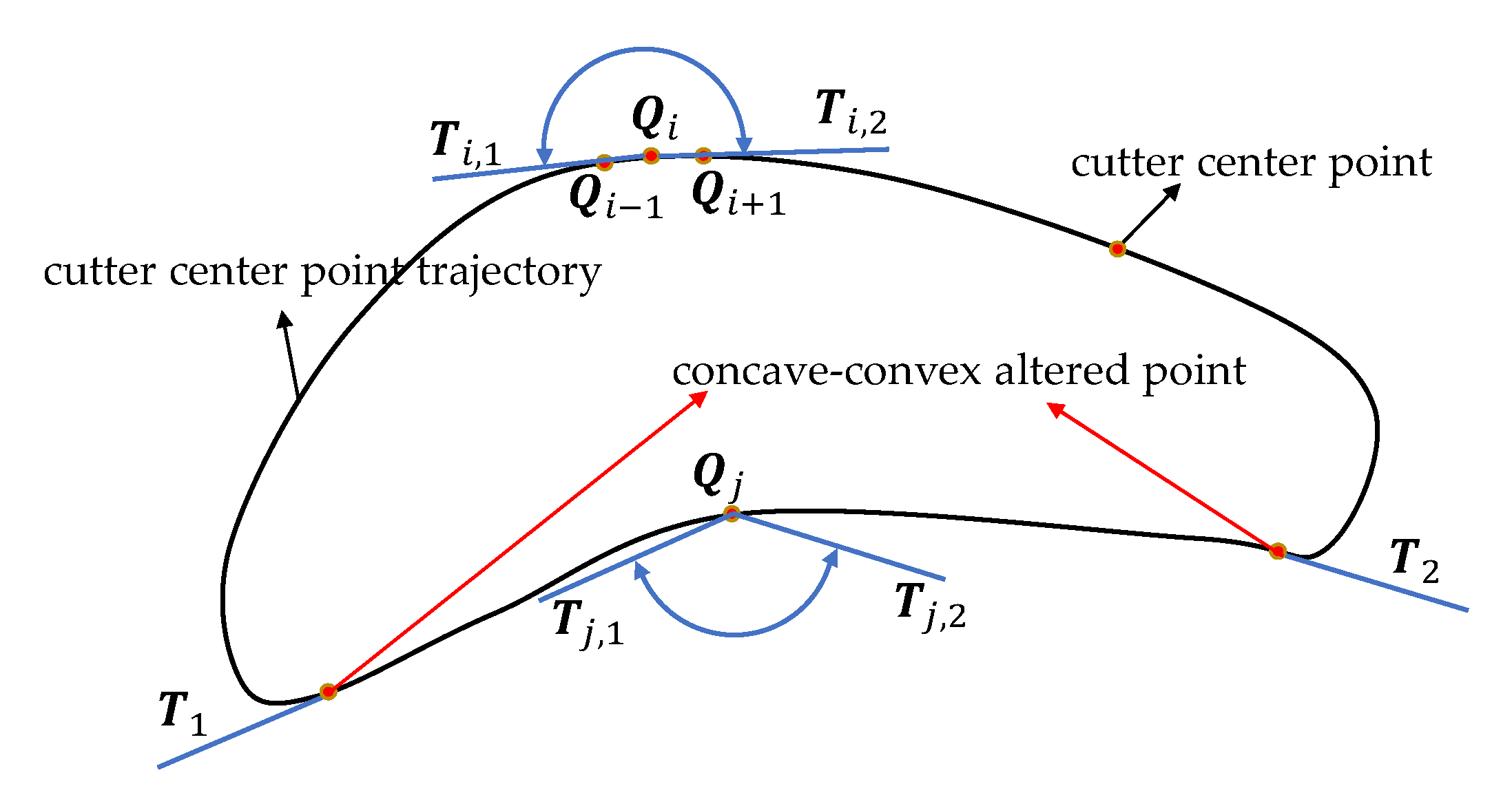
If the cutter center point Q_i is located on the convex side of the cutter center point trajectory, then the limit vectors T_i,1 and T_i,2 can be calculated as

$$\{\begin{array}{c}{\mathit{T}}_{i,1}{=\mathit{Q}}_i-{ \mathit{Q}}_{i-1}\\ {\mathit{T}}_{i,2}{=\mathit{Q}}_{i+1}-{ \mathit{Q}}_i\end{array};$$

(2)

If the cutter center point ${\mathit{Q}}_j$ is located on the concave side of the cutter center point trajectory, then the limit vectors ${\mathit{T}}_{j,1}$ and ${\mathit{T}}_{j,2}$ are respectively equal to the limit vectors ${\mathit{T}}_1$ and ${\mathit{T}}_2$ at two concave-convex altered point. The selection of the limit vectors is shown in the Figure 4.

4.

Adjust the limit vector to avoid interference according to the tool taper angle.

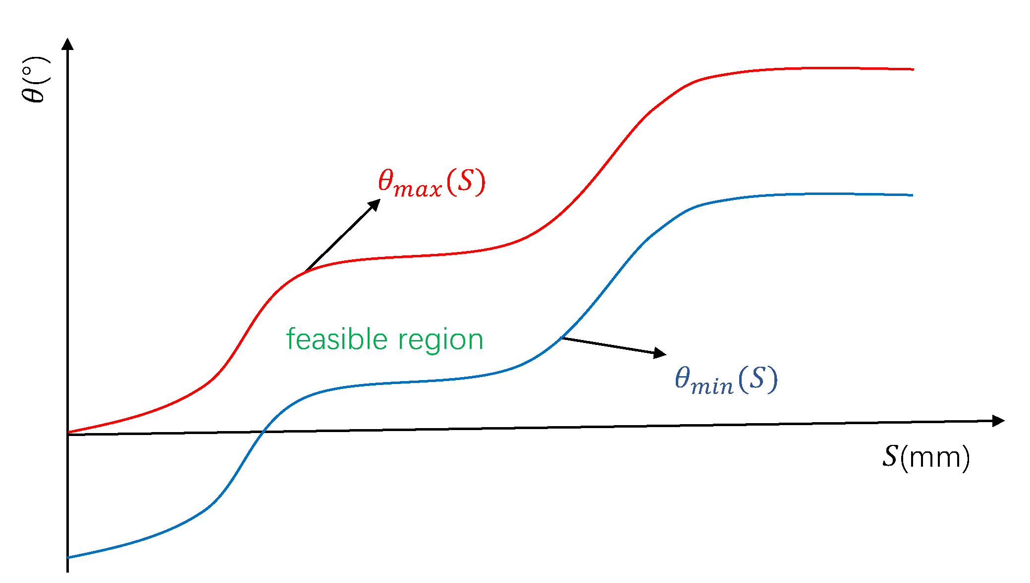
Two limit tool orientations of the current cutter location are obtained. Then, the limit vector is mapped to the $S$-$\theta$ plane to obtain the corresponding two points ${(S}_i{,\theta }_{i,\mathsf{max}})$ and ${(S}_i{,\theta }_{i,\mathsf{min}})$. Finally, traverse all the cutter locations in the section in turn, and two curves ${\theta }_{\mathsf{max}}\left(S\right)$ and ${\theta }_{\mathsf{min}}\left(S\right)$ corresponding to the maximum limit and the minimum limit can be obtained, respectively. The area between the two curves is the feasible region of the tool orientation of this section during machining, as shown in Figure 5. It can be seen that the variation trends of the two limit curves are similar, and the value of $\theta$ increases first and then levels off.

2.2. Decouple the Segmented Tool Orientation

In the scheduling of the segmented tool orientation, to realize the global smoothing of the change of tool orientation, the scheduling at the start of each stage will inevitably incorporate the scheduling results at the end of the previous stage into the constraints. To liberate this limitation, combined with the characteristics of the feasible region of tool orientation, this method gives a clever decoupling idea, so that each sub-stage can be scheduled separately and the overall smoothness will not be affected after merging. The decoupling method of the segmented tool orientation is introduced below.

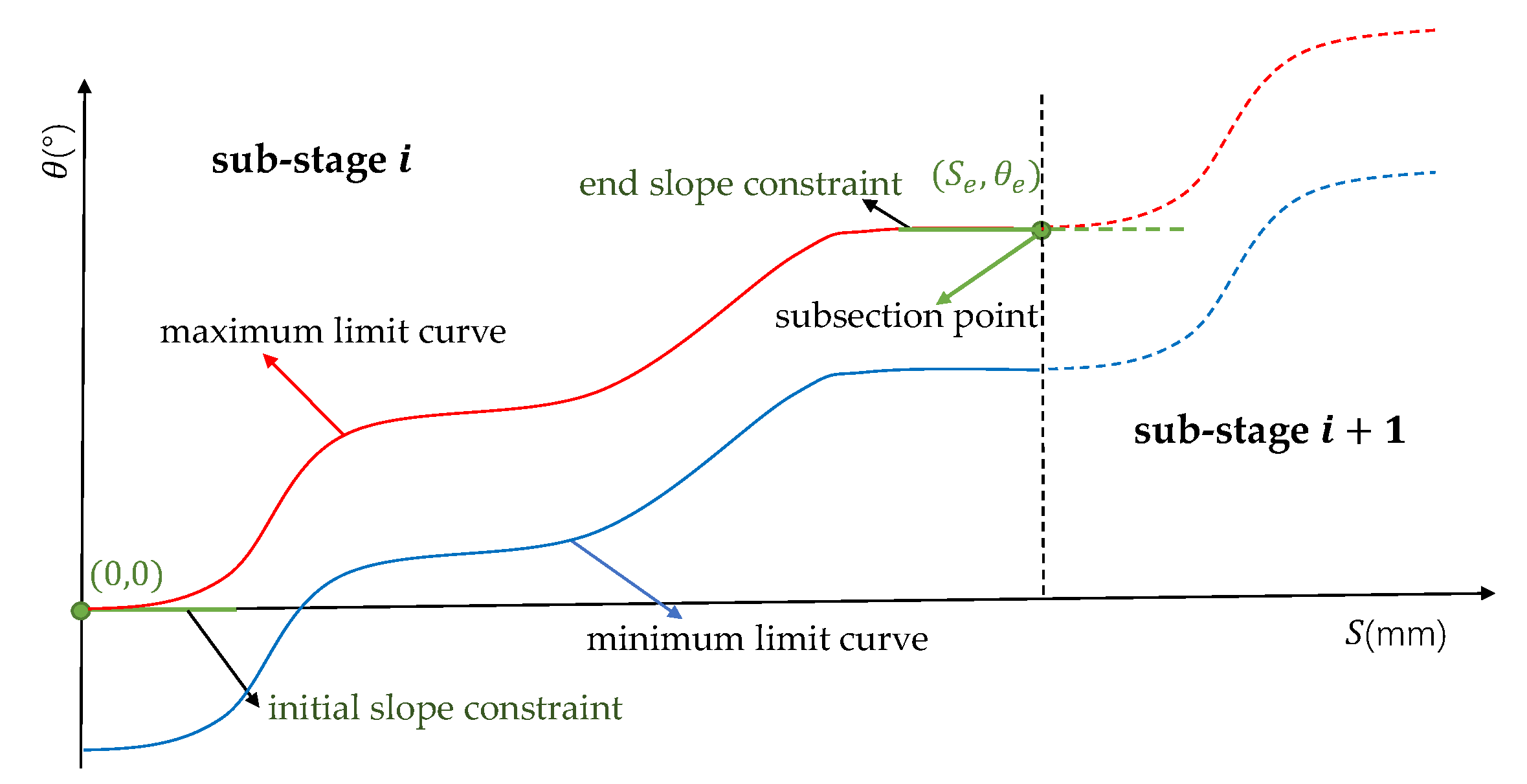
First, except for the first and last toolpaths, this method stipulates that each section is processed from the base point and the tool orientation changes from the base vector. After mapping it to $S$-$\theta$ plane, it is reflected that the tool orientation of each sub-stage starts from (0,0) to an endpoint ${(S}_e{,\theta }_e)$. Since the base vector selects the forward limit position of the tool orientation, the increase of the variable region of the tool orientation is small with the cutter location advances at the beginning of each sub-stage. Therefore, this method limits the tool orientation of each intermediate sub-stage to change from the slope of zero in $S$-$\theta$ plane and reach the end point with the slope of zero at the same time, that is, the transition between each stage is in the state that the angle of the tool orientation remains unchanged. It should be noted that the first and the last segments only need to meet the requirements that the end slope is zero and the starting slope is zero.

In this way, the coupling constraints between the sub-stages to ensure global smoothing are transformed into the constraints within the sub-stages, that is, partial slope constraints, and the decoupling of the segmented tool orientation is realized. The implementation of decoupling method in $S$-$\theta$ plane is shown in Figure 6. Obviously, the internal slope constraint is easier to deal with than the external coupling constraint, so the decoupling work creates favorable conditions for the subsequent tool orientation scheduling.

2.3. Piecewise Linearization Scheduling of Decoupled Tool Orientation

For the tool orientation after piecewise decoupling, it is difficult to reschedule it directly with a smooth curve within the feasible region, because it will inevitably involve the solution of nonlinear constraints or complex objective functions. In order to avoid the complex calculation process, a method is proposed to perform linearization scheduling on the tool orientation first to obtain the monotonic variation of the tool orientation with G0 continuity and then smooth the curve to G2 continuity.

In fact, if the starting point and the ending point of a sub-stage are directly connected in the $S$-$\theta$ plane, and the connected straight line does not exceed the feasible region, then the straight line will undoubtedly be the optimal tool orientation for the machining of this blade section, because it yields zero acceleration. However, the complex surface shape makes the scheduling of most blades unable to meet this condition.

Therefore, the proposed method takes this ideal line in the $S$-$\theta$ plane as the guidance vector and finds the extreme point on the boundary curve of the feasible region as the key point in the rotated coordinate system with the guidance vector as the abscissa axis, and the selected rule is to take the minimum point on the maximum limit curve ${\theta }_{\mathsf{max}}\left(S\right)$ and the maximum point on the minimum limit curve ${\theta }_{\mathsf{min}}\left(S\right)$.

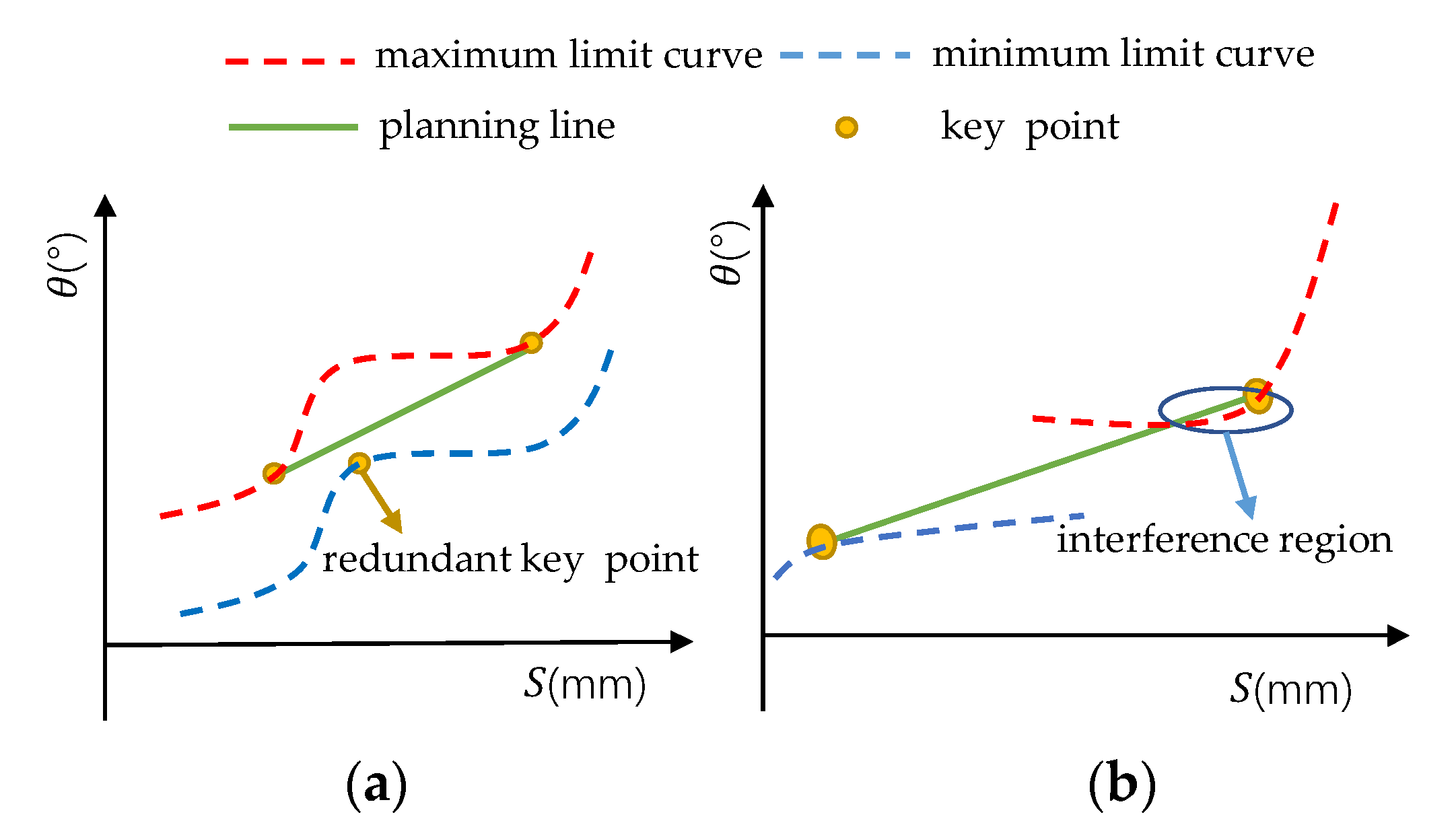
Because the two limit curves do not have a downward trend, the proposed selection method can ensure the monotonicity of the key points, and then ensure the monotonicity of the variation of the tool orientation after linearization scheduling. After obtaining the key points, the position of the key points needs to be adjusted according to different situations. The specific adjustment strategy includes two steps:

The first step is to judge whether there are redundant key points, and if there are, remove them. The redundant key point means that if two adjacent key points on the same boundary curve can be directly connected without traversing unfeasible regions, the key point on the other boundary curve between the two key points is the redundant key point, as shown in Figure 7a.

The second step is to judge whether the connecting line of key points is within the feasible region. If not, move the key points on the maximum limit curve downward and the key points on the minimum limit curve upward to adjust until there is a certain distance between the connecting line and the feasible region. The situation where the connecting line is beyond the feasible region is shown in Figure 7b.

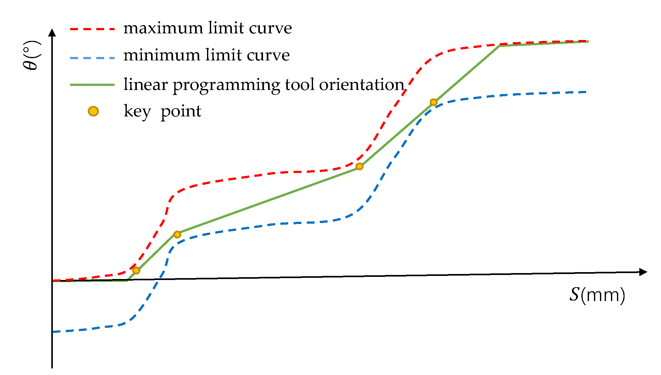
Finally, under the constraint of the slopes at both ends, the adjusted key points are connected by straight line segments in turn, and the tool orientation linearization scheduling with G0 continuity and monotonic variation are realized, as shown in Figure 8.

3. Piecewise Decoupling Tool Orientation Smoothing for Reciprocal Toolpaths with Minimized Acceleration

The linearization scheduling method presented in Section 2 can generate the tool orientation with monotonic variation conveniently; however, the deficiency is that the continuity is merely G0. To improve the continuity of tool orientation variation, a global smoothing method based on Bezier curve is proposed in this section. By assigning control points in the $S$-$\theta$ plane, the proposed method can realize the G2 continuity of tool orientation. Detail of the global smoothing method is presented in following subsections.

3.1. Global Smoothing Based on Bezier Curve

Through piecewise decoupled linearization scheduling of tool orientation, the $S$-$\theta$ plane curve of tool orientation composed of multiple line segments can be obtained, which has G0 continuity. However, the slope and curvature of the curve at the junction point of each line segment are discontinuous, which will lead to sudden changes in the velocity and acceleration of the rotary axis of the machine tool and limit the performance and processing efficiency of the machine tool. Therefore, it is necessary to smooth it with a smooth spline parametric curve. To solve this problem, the Bezier curve is selected as the smooth curve in this method.

In the conventional Bezier curve smoothing method, the error value between the point with maximum curvature on the curve and the corner of the polyline is usually selected as the constraints. However, the smoothing method proposed here is based on the $S$-$\theta$ plane, and the feasible region of tool orientation angle variation is reflected as the distance in the vertical direction in the $S$-$\theta$ plane, so the conventional Bezier curve smoothing method is not applicable. Therefore, a different $S$-$\theta$ plane vertical-direction error constrained curve smoothing method by splicing two cubic Bezier curves is presented and the details are given as follows.

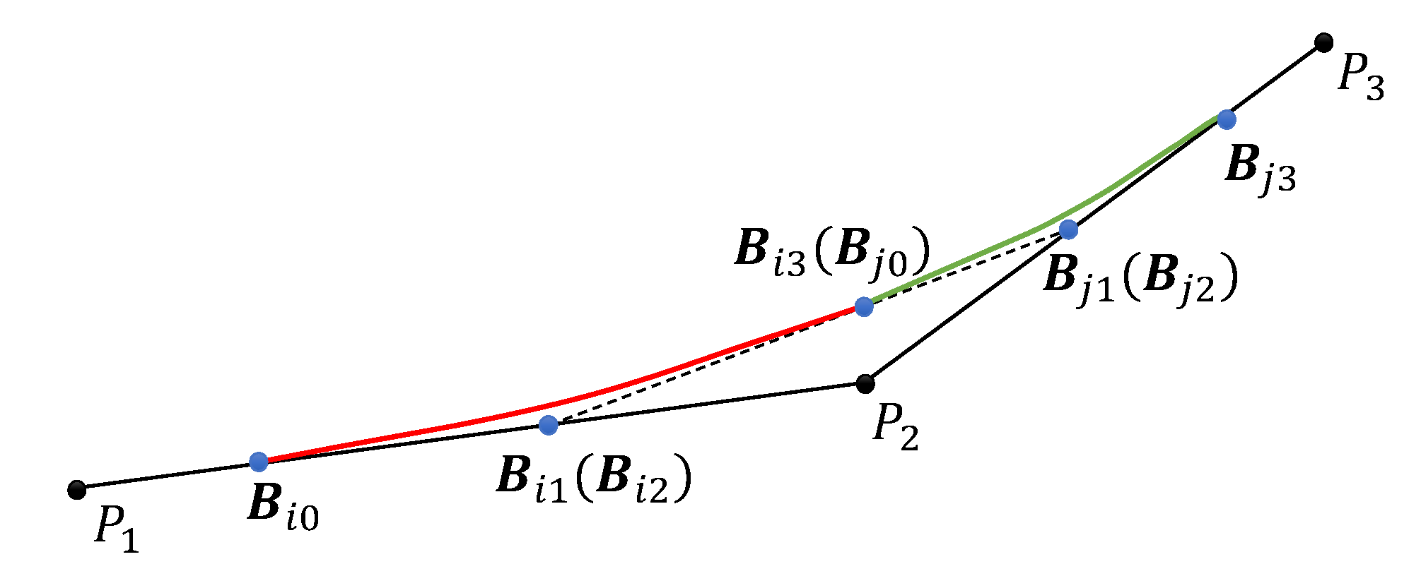
As shown in Figure 9, the corner of two connected linear segments $P_1{P}_2$ and $P_2{P}_3$ are smoothed with a smooth curve composed of two cubic Bezier curves. ${\mathit{B}}_{i0}$, ${\mathit{B}}_{i1}$, ${\mathit{B}}_{i2}$, ${\mathit{B}}_{i3}$, ${\mathit{B}}_{j0}$, ${\mathit{B}}_{j1}$, ${\mathit{B}}_{j2}$, and ${\mathit{B}}_{j3}$ are the control points of the two Bezier curves, respectively, and they are assigned according to the following principles.

1.

B_i3 and B_j0 are coincident and are directly above point P₂;

2.

B_i1 and B_j1 are the intersection points of the straight line that passing through point ${\mathit{B}}_{i3}$ and perpendicular to the angular bisector of $\angle P_1{P}_2{P}_3$, and segments $P_1{P}_2$ and $P_2{P}_3$, respectively. In addition, ${\mathit{B}}_{j2}$ coincides with ${\mathit{B}}_{i1}$, and ${\mathit{B}}_{j2}$ coincides with ${\mathit{B}}_{j1}$, respectively;

3.

${\mathit{B}}_{i0}$ and ${\mathit{B}}_{j3}$ are on the linear segments $P_1{P}_2$ and $P_2{P}_3$, respectively, and the concrete locations are determined by $L_{{\mathit{B}}_{i0}{\mathit{B}}_{i1}}{=L}_{{\mathit{B}}_{i2}{\mathit{B}}_{i3}}$ and $L_{{\mathit{B}}_{j0}{\mathit{B}}_{j1}}{=L}_{{\mathit{B}}_{j2}{\mathit{B}}_{j3}}$, respectively.

According to the characteristics of Bezier curve, it can be proven that the smoothing method can realize the variation of the tool orientation with global G2 continuity.

First, cubic Bezier curve can be expressed as

$$\mathit{B}\left(t\right)=(1-{t)}^3{\mathit{Q}}_0+3t(1-{t)}^2{\mathit{Q}}_1{+3t}^2(1-{t)\mathit{Q}}_2{+t}^3{\mathit{Q}}_3 0 \le t \le 1$$

(3)

where $t$ is curve parameter; ${\mathit{Q}}_0$, ${\mathit{Q}}_1$, ${\mathit{Q}}_2$, and ${\mathit{Q}}_3$ represent four control points.

According to the first-order derivative characteristics of Bezier curve, the slope of the starting point is equal to the slope formed by the first two control points, and the slope of the ending point is equal to the slope formed by the last two control points. For the smooth curve formed by the proposed method, ${\mathit{B}}_{i0}$ and ${\mathit{B}}_{i1}$ are located on segment $P_1{P}_2$; ${\mathit{B}}_{j2}$ and ${\mathit{B}}_{j3}$ are on segment $P_2{P}_3$; ${\mathit{B}}_{i2}$, ${\mathit{B}}_{i3}$, ${\mathit{B}}_{j0}$, and ${\mathit{B}}_{j1}$ are collinear. This means that the first-order derivatives at each connection point are equal, so the global G1 continuity is proven.

Then, the first-order and second-order derivatives of Bezier curve can be calculated as

$${\mathit{B}}^{{}^{\prime }}(t)=3{(1-t)}^2\left({\mathit{Q}}_1-{\mathit{Q}}_0\right)+6t(1-t)\left({\mathit{Q}}_2-{\mathit{Q}}_1\right)+3t^2\left({\mathit{Q}}_3-{\mathit{Q}}_2\right)$$

(4)

$${\mathit{B}}^{{}^{″}}(t)=6(1-t)\left({\mathit{Q}}_2-2{\mathit{Q}}_1+{\mathit{Q}}_0\right)+6t\left({\mathit{Q}}_3-2{\mathit{Q}}_2+{\mathit{Q}}_1\right)$$

(5)

At the endpoints of two Bezier curves, it can be obtained that

$$\{\begin{array}{l}{\mathit{B}}_1^{{}^{\prime }}\left(0\right)=3\left({\mathit{B}}_{i1}-{\mathit{B}}_{i0}\right){,\mathit{B}}_1^{{}^{″}}\left(0\right)=6\left({\mathit{B}}_{i0}-{\mathit{B}}_{i1}\right)\hfill \\ {\mathit{B}}_1^{{}^{\prime }}\left(1\right)=3\left({\mathit{B}}_{i3}-{\mathit{B}}_{i2}\right){,\mathit{B}}_1^{{}^{″}}\left(1\right)=6\left({\mathit{B}}_{i3}-{\mathit{B}}_{i2}\right)\hfill \\ {\mathit{B}}_2^{{}^{\prime }}\left(0\right)=3\left({\mathit{B}}_{j1}-{\mathit{B}}_{j0}\right){,\mathit{B}}_2^{{}^{″}}\left(0\right)=6\left({\mathit{B}}_{j0}-{\mathit{B}}_{j1}\right)\hfill \\ {\mathit{B}}_2^{{}^{\prime }}\left(1\right)=3\left({\mathit{B}}_{j3}-{\mathit{B}}_{j2}\right){,\mathit{B}}_2^{{}^{″}}\left(1\right)=6\left({\mathit{B}}_{j3}-{\mathit{B}}_{j2}\right) \hfill \end{array}.$$

(6)

The curvature at any point on the cubic Bezier curve is

$$\kappa \left(t\right)=\frac{{\mathit{B}}^{{}^{\prime }}\left(t\right){\times \mathit{B}}^{{}^{″}}\left(t\right)}{{\Vert {\mathit{B}}^{\prime }\left(t\right)\Vert }^3}.$$

(7)

Substituting Equation (6) into Equation (7), the curvature at each connecting point of the curve can be obtained as

$$\{\begin{array}{l}{\kappa }_1\left(0\right)=0\hfill \\ {\kappa }_1\left(1\right){=\kappa }_2\left(0\right)=0\hfill \\ {\kappa }_2\left(1\right)=0\hfill \end{array}.$$

(8)

Because the curvatures of the line segments are also 0, the smoothing method realizes the continuous variation of curvature; therefore, the G2 continuity is proved.

3.2. Assignment of Control Points for Smooth Curve

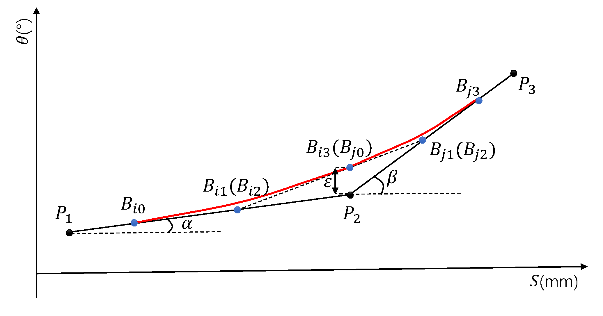
After determining the form of the smoothing curve, the smoothing problem is transformed into the calculation of the positions of the control points. Assuming that there are two connected line segments $P_1{P}_2$ and $P_2{P}_3$ in $S$-$\theta$ plane, and the coordinate values ${(S}_1{,\theta }_1)$, ${(S}_2{,\theta }_2)$, and ${(S}_3{,\theta }_3)$ of the three endpoints are known, then the included angle between these two segments and the horizontal line, denoted by $\alpha$ and $\beta$ which can be seen in Figure 9, can be obtained. When smoothing a corner, a total of five control point coordinates need to be calculated, as shown in Figure 10.

Taking $\epsilon$, which is obtained by subtracting the ordinates of ${\mathit{B}}_{i3}$ and $P_2$, as the independent variable, the coordinates of the five control points can be given by the following formula:

$$\{\begin{array}{l}{\mathit{B}}_{i0}=\left(S_2+\frac{\epsilon \cos \alpha (\cos \alpha +\cos \beta )}{\sin (\beta -\alpha )},{\theta }_2+\frac{\epsilon \sin \alpha (\cos \alpha +\cos \beta )}{\sin (\beta -\alpha )}\right)\hfill \\ {\mathit{B}}_{i1}=\left(S_2+\frac{\epsilon }{\tan \alpha -\tan {\beta }^{\prime }},{\theta }_2+\frac{\epsilon \tan \alpha }{\tan \alpha -\tan \beta }\right)\hfill \\ {\mathit{B}}_{i3}=\left(S_2,{\theta }_2+\epsilon \right)\hfill \\ {\mathit{B}}_{j1}=\left(S_2+\frac{\epsilon }{\tan \gamma -\tan {\beta }^{\prime }},{\theta }_2+\frac{\epsilon \tan \gamma }{\tan \gamma -\tan \beta }\right)\hfill \\ {\mathit{B}}_{j3}=\left(S_2+\frac{\epsilon \cos \gamma (\cos \gamma +\cos \beta )}{\sin (\beta -\gamma )},{\theta }_2+\frac{\epsilon \sin \gamma (\cos \gamma +\cos \beta )}{\sin (\beta -\gamma )}\right)\hfill \end{array}$$

(9)

where $\gamma =\frac{\alpha +\beta }{2}$.

In order to make the smoothed tool orientation variation curve yield as little acceleration as possible, $\epsilon$ should be taken as large as possible. However, two constraints that cannot be ignored restrict the value of $\epsilon$.

First, the smoothed curve cannot exceed the feasible region, that is, the boundary constraint. Second, the distance between the two ends of the smooth curve and the endpoint of the corresponding line segment cannot be less than half of the length of the line segment, which is forced to ensure that the two adjacent smooth segments will not intersect with each other.

In the range from the midpoint of segment $P_1{P}_2$ to the midpoint of segment $P_2{P}_3$, the minimum distance between the feasible region boundary and the segment is marked as ${\epsilon }_0$. when $\epsilon \le { \epsilon }_0$, it is obvious that the first constraint is guaranteed. As for the second constraint considering intersection, the following formula can be used

$$\{\begin{array}{c}{d}_1 \le \frac{l_1}{2}\\ d_2 \le \frac{l_2}{2}\end{array}$$

(10)

where $d_1$ represents the distance between point ${\mathit{B}}_{i0}$ and point $P_2$, $d_2$ represents the distance between point ${\mathit{B}}_{j3}$ and point $P_2$, $l_1$ and $l_2$ represent the length of line segments $P_1{P}_2$ and $P_2{P}_3$, respectively.

According to the coordinates of control points, $d_1$ and $d_2$ can be calculated as

$$\{\begin{array}{c}{d}_1=\frac{\epsilon \left(\cos \alpha +\cos \beta \right)}{\sin (\beta -\alpha )}\\ d_2=\frac{\epsilon \left(\cos \gamma +\cos \beta \right)}{\sin (\beta -\gamma )}\end{array}.$$

(11)

Substituting Equation (11) into the constraint, the constraint of $\epsilon$ can be expressed as

$$\{\begin{array}{c}\epsilon \le \frac{l_1\sin (\beta -\alpha )}{2\left(\cos \alpha +\cos \beta \right)}\\ \epsilon \le \frac{l_2\sin (\beta -\gamma )}{2\left(\cos \gamma +\cos \beta \right)}\end{array}.$$

(12)

From the above, we can get that the maximum value $\epsilon$ can be taken under the following constraint

$$\epsilon =\min \left\{{\epsilon }_0,\frac{l_1\sin (\beta -\alpha )}{2(\cos \alpha +\cos \beta )},\frac{l_2\sin (\beta -\gamma )}{2(\cos \gamma +\cos \beta )}\right\}.$$

(13)

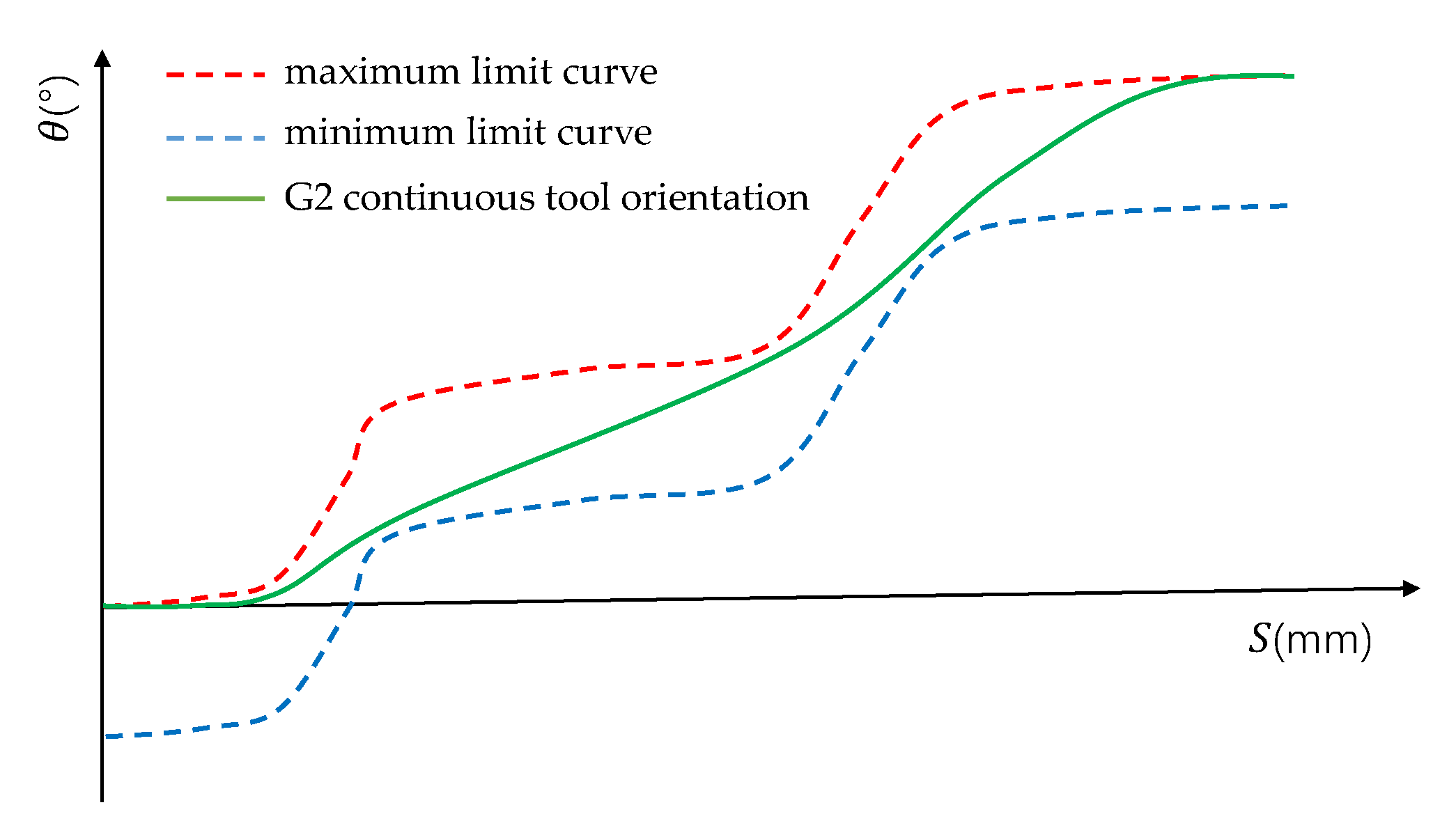
When the value of $\epsilon$ is determined, it means that the coordinates of the five control points are determined according to Equation (9), and then they are substituted into the cubic Bezier curve equation to obtain the smooth curve of the line segments. After smoothing all line segments in this way, the tool orientation variation curve after linearization scheduling can be smoothed into a monotonic interference-free tool orientation variation curve with global G2 continuity, as shown in Figure 11.

According to the base vector and the tool orientation variation curve, the tool orientation of each cutter location in this sub-stage can be obtained. Then, according to Equation (1), the new tool tip coordinates can be inversely obtained. Finally, the new machining code can be obtained by completing all sub-stages in turn. The overall flow chart of tool orientation scheduling is shown in Figure 12.

4. Simulation and Experiment

In this section, simulation and experimental tests are conducted to verify the effectiveness of the proposed method. The comparison simulation tests with a representative quaternion interpolation method are conducted to evaluate the superiority of the proposed method. Finally, the results are analyzed and discussed based on comparison of the test data.

4.1. Simulation and Experiment Setup

The simulation object is a blade which is actually machined in the factory, and the machining toolpaths are extracted through its machining code which is generated by a commercial CAM software. To verify the effectiveness of the proposed method, it is used to schedule the tool orientation of the blade machining. To verify the superiority of the proposed method, the representative quaternion interpolation method proposed in reference [16] is selected for comparative testing. In order to intuitively analyze the variation of tool orientation, we analyze the tool orientation scheduled by different methods in the direction which perpendicular to the stratification plane. In addition, in order to analyze the motion state of each axis of the machine tool with different toolpaths, we used the same feedrate to test the three toolpaths. The motion acceleration and velocity of each axis is compared to further verify the effectiveness and superiority of the proposed method.

In order to verify the feasibility of the proposed method, the experimental tests were carried out on the StarragLX451 machine tool, and the tool used was a ball-end milling cutter with a radius of 8 mm. The type of the machine tool is rotary table and pivoting spindle head. The detailed technical data of the machine tool are shown in

Table 1. The technical data of the machine tool.

Parameter	Value	Unit
Max. distance between centers	2805	mm
Swing Diameter	650	mm
Strokes of X-axis	2800	mm
Strokes of Y-axis	660	mm
Strokes of Z-axis	600	mm
Strokes of A-axis	360	degree
Strokes of B-axis	+/−87	degree
Standard/Max number of Tools	24/62	−
Tool chancing time	8	sec

. The swing angle of the machine spindle (B-axis) was fixed as 5 degrees to test the four-axis machining of the blade. The experimental environment is shown in Figure 13. The material of the blade is 12Cr12Mo steel, and the machining region is the root of the blade. Figure 14 shows the blade used for experimental machining.

4.2. Results and Discussion

The tool orientation in the direction perpendicular to the stratification plane when the blade is machined according to the original code is shown in Figure 15a. It is obvious that the tool orientation suffers from frequent reciprocal swing, and the tool orientation changes violently at the locations around the blade edges.

The tool orientation obtained by quaternion interpolation planning is shown in Figure 15b. It can be seen that the compared method can also obtain smoothly changing tool orientation, but the reciprocating variation of tool orientation still exists.

After segmentation, decoupling, linearization scheduling, and curve smoothing, the tool orientation in the direction of vertical rotary axis which is scheduled by the proposed method is shown in Figure 15c. It can be seen that the tool orientation after scheduling has no reciprocal swing, and the variation of tool orientation is steadier.

Based on different methods, the comparison of motion state of the rotary axis is shown in Figure 16. Compared with the original processing method, the proposed method and the compared method can reduce the extreme value and fluctuation of the velocity, and greatly reduce the acceleration fluctuation. Compared with the representative quaternion interpolation method, the proposed method can lower the velocity and acceleration of the rotary axis in a larger extent. Compared with the compared method, the proposed method can reduce the extreme value of the velocity and acceleration of the rotary axis by 38.1% and 72.9%, respectively.

In fact, although the tool orientation scheduling mainly focuses on the rotary axis, the motion state of each translational axis of the machine tool after scheduling has also been improved to varying degrees. Figure 17 shows the comparison of velocity and acceleration of the three translational axes. It can be seen that the proposed method and the compared method can also reduce the extreme value and fluctuation of the velocity and acceleration of the three translational axes. Compared with the comparison method, the optimization ratios of the extreme value of the velocity and acceleration of the three translational axes are shown in

Table 2. Optimization ratios of the proposed method compared with the compared method.

Axis	Extreme Value of Velocity	Extreme Value of Acceleration
X-axis	6.3%	10.6%
Y-axis	46.2%	71.4%
Z-axis	69.2%	83.7%

.

In the experimental tests, the root of the blade is machined with the original machining code and the new machining code generated by the proposed method, and the results are shown in Figure 18. It can be seen that compared with the original toolpaths, the toolpaths scheduled by the proposed method results in the similar tool marks and machining quality. However, compared with the original method, the processing efficiency of the proposed method is improved by 24.5%. This is because the velocity and acceleration of each axis are constrained by the dynamic characteristic of the machine tool, so the feedrate has to be reduced to submit to the constraints when machining with the original method. In contrast, the new machining code can keep the feedrate at a high fixed value, which is a benefit from lower maximum axis velocities and accelerations after scheduling. In fact, the proposed method can not only improve the processing efficiency, but also theoretically extend the operating time of the tool. Compared with a fixed inclination angle, the inclination angle of the tool scheduled by the proposed method changes smoothly within the allowable range, which makes the tool wear more uniform.

Simulation and experimental tests show the effectiveness and superiority of the proposed method. Simulation tests verify that the proposed method can effectively reduce the velocity and acceleration fluctuation of each axis of the machine tool, and the effect is better than the classical quaternion interpolation method. It means that under the same machine-tool performance constraints, the scheduled toolpaths can adopt a higher feedrate. The results of experimental tests further prove this inference. The machining duration of the toolpaths scheduled by the proposed method is shorter the original toolpaths. In addition, compared with the representative quaternion interpolation method, the proposed method performs better in the optimization of the motion state of the translational axis.

5. Conclusions

In this paper, a new tool orientation re-scheduling method for four-axis machining is proposed, and it is aimed at reciprocal machining of blades. The main work includes completing the piecewise decoupling linearization scheduling of tool orientation in the $S$-$\theta$ plane and smoothing the curve of tool orientation variation after linearization scheduling. The whole machining process is first divided into similar sub-stages, then the $S$-$\theta$ plane is constructed and the feasible range of tool orientation is calculated in this plane. After that, through decoupling and linearization scheduling, the tool orientation with monotonicity and G0 continuity is obtained. Finally, the smoothing curve is used to smooth the linearization scheduling results, and the smoothness of the tool orientation is improved to global G2 continuity. This smoothing process is based on the assignment of control points without involving complex calculation.

The feasibility and superiority of this method are verified by simulation and experiment. Compared with the current mainstream processing methods, this method can eliminate the frequent swing of the rotary axis of the machine tool, reduce the velocity and acceleration fluctuation of each axis of the machine tool, and improve the processing efficiency. The results show that the machining efficiency of the blade is improved by 24.5%, due to the reduction of the requirement on highest feed-axis kinematics parameters after rescheduling. Compared with most existing tool orientation scheduling methods, this method considers the reverse clearance of machine tool structure and can realize the monotonic variation of tool orientation. In addition, the whole scheduling process does not involve complex iterative calculation and optimization solutions, which greatly reduces the calculation difficulty of tool orientation scheduling.