Improving Industrial Robot Positioning Accuracy to the Microscale Using Machine Learning Method

Abstract

Positioning accuracy in robotics is a key issue for the manufacturing process. One of the possible ways to achieve high accuracy is the implementation of machine learning (ML), which allows robots to learn from their own practical experience and find the best way to perform the prescribed operation. Usually, accuracy improvement methods cover the generation of a positioning error map for the whole robot workspace, providing corresponding correction models. However, most practical cases require extremely high positioning accuracy only at a few essential points on the trajectory. This paper provides a methodology for the online deep Q-learning-based approach intended to increase positioning accuracy at key points by analyzing experimentally predetermined robot properties and their impact on overall accuracy. Using the KUKA-YouBot robot as a test system, we perform accuracy measurement experiments in the following three axes: (i) after a long operational break, (ii) using different loads, and (iii) at different speeds. To use this data for ML, the relationships between the robot’s operating time from switching on, load, and positioning accuracy are defined. In addition, the gripper vibrations are evaluated when the robot arm moves at various speeds in vertical and horizontal planes. It is found that the robot’s degrees of freedom (DOFs) clearances are significantly influenced by operational heat, which affects its static and dynamic accuracy. Implementation of the proposed ML-based compensation method resulted in a positioning error decrease at the trajectory key points by more than 30%.

1. Introduction

Robots are used in various processes, including manufacturing, entertainment, services, and scientific research. To maintain a technical edge and thereby remain competitive, more and more businesses are applying advanced technology and programming solutions to their operational processes [1]. Such a wide application encourages the development of universal robotic systems and requires research of their capabilities and performance characteristics.

In general, industrial robots provide high-level static and dynamic positioning accuracy. Nevertheless, they must be maintained to ensure that they continue to meet the conditions for which they have been programmed and in which they operate [2]. Therefore, for each specific task, it is important to determine the following: (i) positioning accuracy (positioning error between stated and the real position of arm end effector); (ii) repeatability (positioning error between real positions of arm end effector performing repeating movements); (iii) other parameters, which are considered to be unique characteristics of the particular machine [3]. Positioning accuracy depends on a number of actions including, but not restricted to the following: (i) the parameters of the drives guiding the robot’s movements; (ii) tolerances in manufacturing parts of the machinery; (iii) tolerances due to the articulation of the robot’s chains [4]; (iv) control algorithms [5,6]; (v) dynamic properties of the mobile platform [7,8], and (vi) robot arm properties [9,10]. Each of the factors may become important for the accuracy of the robot, depending on its type, lifting capacity, and operational conditions [4]. Due to the complex nature of robots, the increasing positioning accuracy of robotic installations develops challenging tasks. The positioning errors in offline mode can be determined using special algorithms [11] and mathematical models [12,13,14,15]. Common positioning accuracy problems in path and trajectory planning can be resolved by improving offline programming software when the code for a robot is generated automatically or by implementing online feedback [16,17,18,19,20]. However, typical compensation methods are limited by the chaotic nature of the positioning errors. Therefore, more adaptive methods, such as machine learning (ML), can increase positioning accuracy by compensating for positioning errors in particular cases [21,22]. Advances in ML with respect to simple error compensation are in the accountancy of feature-chaotic robot error distribution about positioning points. ML ensures respect for robot fluctuation and fits into the prescribed tolerance field. There are a few cases [23,24,25,26] of ML approaches compensating for the positioning errors. Chen and Zhang developed an ML kinematics-based positioning error compensation method for high-precision mechanical machining operations [26]. This positioning error compensation method provided good results, but it contains sophisticated procedures due to its complexity and use of excessive data. More to say, it combines the following: analytical modeling; extended Kalman filtering; spatial interpolation algorithm; an adaptive mesh division algorithm, and an inverse distance weighted interpolation algorithm. To use it at a few trajectory points, this method becomes too costly.

Moreover, ML could be implemented to improve the trajectory-planning process [27,28,29] or reduce vibrations [30,31].

The main aim of our research is to create a methodology to increase industrial robot positioning accuracy and minimize robot end-of-arm vibrations by applying ML in online mode. This methodology will be used to compensate for positioning errors by shifting the destination point or altering the moving velocity of the end-of-arm reference point before defining the forward kinematic task. The method is focused on destination point approach accuracy in defined arbitrary robot positions. Moreover, our proposed approach suits well for industrial robots with typically closed controllers since position correction is performed externally with respect to the robot controller; thus, modified motion commands to target coordinates are processed in a standard way.

2. Concept of Research

This paper focused on creating a universal methodology for most types of industrial robots, which can increase positioning accuracy at the robot trajectory endpoints. One of the pillars of ML is mathematical optimization, which involves the numerical computation of parameters for a system designed to make decisions based on unseen data [32,33,34]. While the ML procedure is based on existing data collection, such a method all the time remains retrospective and reflects errors in previous applications with corresponding load cases. The use of the robot for precise machining or assembly operations requires data about the vibration level and settling time. This will be critically important in addition to static positioning error values and directions. The ML procedure enables a decrease in positioning error values, and end-of-arm vibration influences the resulting accuracy. Nevertheless, the robot workspace mapping procedure, which provides error values and direction at any point of the workspace, all the time remains inaccurate for each particular case.

It is possible to calculate optimal parameters for a given learning problem using currently available data [35]. The collection of data required for ML is a complex process, defined by the robot design, its characteristics, and the aim of ML implementation.

The procedure of implementing our proposed ML method is divided into the following three phases: (i) initial preparation, (ii) positioning task formulation, and (iii) optimization (Figure 1).

The success of the ML procedure depends on the quantity and quality of data generated during initial preparation. This phase includes experiments for the definition of the main robot’s characteristics, such as positioning accuracy, reference point vibration level, statistical evaluation, and analysis of obtained data. The initial preparation procedure should be performed for all robot trajectory points of interest. This procedure must be repeated in cases of mechanical wear, change of tool configuration, or essential variation of environmental conditions.

The obtained data shows the technical conditions of the robot since these data consist of a set of dependencies between positioning errors, vibration level, reference point position, operating time, robot speed, and load. In the general case, these dependencies can be expressed as follows:

$$\{\begin{array}{c}{\mathsf{\Delta }}_{x,y,z}=F\left(x,y,z,V,M,t_{op}\right)\\ {\epsilon }_{x,y,z}=F\left(x,y,z,V,M\right)\end{array}$$

(1)

where: Δ_x,y,z is the overall positioning error, ε_x,y,z is the overall level of reference point vibrations, x y z are coordinates of robot reference point, V is the speed of reference point, M is load, t_op is the time from the moment when a robot was switched on.

The second phase of our proposed ML method is the Formulation of the positioning task. In this phase, it is necessary to define the required position and speed of the reference point (x y z, V) and load (M). Moreover, it is necessary to specify the following limitations: acceptable overall positioning error Δ_min, and overall vibration level of reference point ε_min. In general, case limitations can be identified as follows:

$$\{\begin{array}{c}{\mathsf{\Delta }}_{x,y,z}\le {\mathsf{\Delta }}_{min}\\ {\epsilon }_{x,y,z}\le {\epsilon }_{min}\end{array}$$

(2)

Moreover, to ensure stable operation of the ML algorithm and avoid looping in the algorithm (when the desired accuracy cannot be achieved), it is necessary to include a parameter specifying the maximum number of iterations k_max.

The third phase is the Optimization procedure, which contains the cycle during which the optimization algorithm is used to obtain the most suitable compensation parameters in order to achieve the required positioning accuracy and an acceptable level of reference point vibrations.

The ML algorithm runs with each new positioning task; ML selects compensation parameters and predicts the expected positioning error Δ_x,y,z, and reference point vibration level. This prediction is based on experimentally defined data obtained during the Initial preparation phase. After defining the expected positioning error Δ_x,y,z and reference point vibration level ε_x,y,z, their values are compared with the limitations. If positioning error and reference point vibration level correspond to the limitations of Equation (2), then modified coordinates of the required reference point position and speed are transferred to the robot controller. In case if results do not correspond to the limitations, the data is saved and checked if the maximum number of iterations k_max are reached. The optimization of compensation parameters is performed many times until the limit of iterations is reached. In case if the maximum number of iterations is not achieved, the program selects the best result from all previous iterations.

Deep q-Learning Algorithm

The deep Q-learning algorithm was implemented to realize the mentioned ML procedure. The advantage of this algorithm in comparison to others is emphasized due to its efficiency in similar problems and its relatively simple implementation [36,37,38]. The deep Q-learning algorithm combines the Q-learning algorithm and a deep artificial neural network. The idea of Q-learning is based on the perception of the environment and state to take respective actions in order to achieve the maximum reward. A neural network enables the algorithm to operate in a much larger environment and optimize calculations procedure by enabling approximation features. It allows the algorithm to observe the pattern in the environment and discover the optimal sequences of actions instead of calculating and evaluating each state and the value of each action at each point in the environment. The same principle was used to optimize the definition of the algorithm loss function. We used the stochastic gradient descent method (SGD) [35] to define the function by the theoretical gradient calculated from randomly selected data points instead of calculating the actual gradient from the entire dataset. Such an approach diminishes the dependency of obtained data from strong dataset influence on functional distribution. Other parameters of the implemented algorithm were selected experimentally by evaluating their impact on positioning accuracy after many trials in a separate study. The configuration of the algorithm used in this study is provided in

Table 1. Parameters of the implemented algorithm.

Parameter	Activation Function	Optimizer	Hidden Neurons	Hidden Layers	Replay Memory	Temperature
Value	Softsign	SGD	37	1	100,000	70

.

The parameters within Table 1 were defined through the experimental running of the algorithm. Process activation through the Softsign procedure corresponds to the robot learning mode, while there are possibilities for other functions. The activation margin (sensitivity to the activation condition) needs redefinition; the ML process converges correctly and, within 1000 iterations, achieves learning process influence saturation. The implemented optimizer—SGD—corresponds to our purposes and achieves the prescribed result. A number of neurons is chosen according to the desired process parameter resolution, and the number of hidden layers is naturally chosen as one according to the dimensionality of the ML process. The amount of replay memory is defined by the experimental test, and it occurs outside our paper scope as well as the temperature parameter.

Furthermore, this paper provides a detailed methodology for experimental research and data collection for ML.

3. Experimental Research

3.1. Experimental Setup

The experiments were performed using the KUKA-YouBot robot (KUKA, Augsburg, Germany) as an industrial robot testbench; it was fixed to a special stable base. The robot’s geometric parameters and main characteristics are provided in

Table 2. General characteristics KUKA-YoubBot arm [39].

General Information		Axes Motion Range, Speed
Serial kinematics	5 axes	Axis 0 (A0)	+/−169°, 90°/s
Height	655 mm	Axis 1 (A1)	+90°/−65°, 90°/s
Work envelope	0.513 m3	Axis 2 (A2)	+146°/−151°, 90°/s
Weight	6.3 kg	Axis 3 (A3)	+/−102°, 90°/s
Payload	0.5 kg	Axis 4 (A4)	+/−167°, 90°/s

[39]. Positions of the robot’s gripper were detected using two USB cameras with a resolution of 1920 × 1080, a checkerboard matrix of 4 × 8 mm size, and a user-defined function, implementing the detect Checkerboard Points procedure in MatLab (Figure 2). According to [40], the use of such a measurement method can ensure an average measurement deviation better than 0.0004 mm.

The cameras were fixed by a special holder positioned at a 90° angle relative to each other to resolve spatial coordinates of the end-of-arm reference point (Figure 2b). The holder with attached cameras was screwed to the same base as the robot. Two special checkerboard patterns (identification marks for cameras) were attached to the gripper (Figure 2b,c).

Absolute vibration accelerations of the end-of-arm reference point were measured using industrial accelerometers Ini 603C01 (PCB Piezotronics, Depew, NY, USA) with a measurement range of 0.5~10,000 Hz and an acceleration limit of 51 g. Accelerometers were attached to the gripper in three perpendicular directions, as shown in Figure 2c. Signals from accelerometers were collected using the data acquisition system USB-4432 (National Instruments, Austin, TX, USA).

Ambient temperature was measured using a digital thermometer MWF-DT-616CT (CEM Corporation, Matthews, NC, USA), with a resolution of 0.1 C. Loads were weighted using Silver crest HG01025 (Silvercrest, Corona, CA, USA) scales, with a resolution of 0.001 kg. For the determination of the required warm-up time, the unloaded robot moves at 50% of the max joint speed (which is 90°/s for all axes) to the trajectory endpoint (Figure 3), rotating joints by the following angles: φ₀—90°, φ₁—15.2°, φ₂—45.7°, φ₃—44.2°, φ₄—20°, and backward. Then the robot returns to the start position, waits for 3 s, and the image of the checkerboard matrix is captured. The experiment trials took place after long operation breaks of 12, 2, and 1 h. In the case of a 2- and 1-h operation break, the warming procedure was applied before the experiment. Firstly, the robot was warmed up using a 30 min warming program and 2- and 1-h operation breaks afterward, correspondingly.

The positioning accuracy measurements were performed in the same conditions, but in this case, experiments were carried out with 10%, 50%, and 100% of the maximum joint speed, without load, and loaded by 0.250 kg and 0.500 kg weights. Each measurement was repeated 20 times.

The proposed methodology for the online ML procedure was tested for 2 different robot configurations, imitating the pick-and-place task. In each individual case, using our online ML method, the procedure can be performed at any chosen position in the robot workspace.

3.2. Evaluation of the End-of-Arm Reference Point Vibrations

The dynamic parameters of the robot—the end-of-arm reference point vibration level and settling time when the robot stops at the desired positions—were evaluated using accelerometers (Figure 2c). There are the following three parameters for measuring vibrations: displacement, velocity, and acceleration. The evaluation of vibration acceleration provides the best sensitivity in higher frequencies and suits well for evaluating impacts caused by bearing damage, abnormal gears, and noise. Moreover, this method is recommended when it is necessary to evaluate forces and stresses acting on or rotating parts. Moreover, measurements of acceleration do not require reference points. Therefore, it is more convenient for industrial robots.

The measurements were carried out at the following three different speeds of the joints of the robot: at 10%, 50%, and 100% of the maximum (90°/s) speed of the joint, using the same robot movement trajectory as shown in Figure 3. The measurement was repeated three times.

The separate DOF effect on the robot end-of-arm vibrations was evaluated by rotating each robot joint separately. For this purpose, joints I-V at coordinates φ₀–φ₄ were rotated clockwise by a 60° angle at maximum (90°/s) speed from the start position Figure 4. The end-of-arm reference point vibrations were measured after the movement of each joint by 60° at a maximum (90°/s) speed. After 10 s, the joints were rotated back to the start position. Measurements were performed when the robot moved in forward and backward directions, and the procedure was repeated three times.

To define the impact of joint I (coordinate φ₀, Figure 5) on robot end-of-arm vibrations, joint I was rotated at 60° from the start position, and the vibrations were measured. The vibrations at the following two start positions were evaluated: (i) fully extended position (Figure 5a); (ii) compacted position (Figure 5b).

In a fully extended position robot’s own weight fully loads joint I. Other joints remain unloaded and stay in a singularity position. The compacted robot position is represented by the situation when joint I is loaded by half of the own weight of other links.

All vibration measurements were performed according to the flowchart provided in Figure 6.

Signals from three accelerometers were recorded continuously during robot movement between the endpoints of the trajectory. Later acquired data were processed offline (Figure 7), defining transient processes due to robot stops at the trajectory endpoints.

Main parameters (end-of-arm reference point maximum peak-to-peak vibration amplitude, settling time) were extracted from raw data, processed statistically, grouped according to testing conditions, and represented in graphical form.

3.3. Calculations

Overall positioning accuracy from measurements in separate axes was evaluated according to the methodology provided by ISO 9283:1998 [41]. It defines positioning accuracy AP_p as the deviation between a reference position and the mean of attained positions while approaching reference positions from the same direction as follows:

$$A{P}_p=\sqrt{{(\overline{x}-x_c)}^2+{(\overline{y}-y_c)}^2+{(\overline{z}-z_c)}^2},$$

(3)

where $x_c$ $y_c$ $z_c$ are coordinates of the prescribed end-of-arm reference point position, and $\overline{x}$, $\overline{y}$, $\overline{z}$ are mean values of the resulting position.

General robot positioning error consists of accumulated values from all errors, and it is an object of ML-obtained compensation. General error from three-axis measurements for the experiments in 1, 2, and 12 h evaluated using the simplified equation, since target position defined as $x_c=0$, $y_c=0$ and $z_c=0$ as follows:

$$A{P}_p=\sqrt{{(\overline{x})}^2+{(\overline{y})}^2+{(\overline{z})}^2}.$$

(4)

where $\overline{x}$ $\overline{y}$ $\overline{z}$ are calculated from experimental data as follows:

$$\overline{x}=\frac{1}{n}{{\displaystyle \sum }}_{j-1}^n{x}_j , \overline{y}=\frac{1}{n}{{\displaystyle \sum }}_{j-1}^n{y}_j , \overline{z}=\frac{1}{n}{{\displaystyle \sum }}_{j-1}^n{z}_j,$$

(5)

where: $x_j$ $y_j$ $z_j$ are coordinates of the resulting position, and n is the measurement cycle number.

Robot positioning repeatability RP_l, also was evaluated using the methodology proposed in ISO 9283:1998. According to it, RP_l value is the radius of the sphere that defines the closeness of an attained position after n attempts to achieve the same position from the same direction as follows:

$$R{P}_l=\overline{l}+3S_l,$$

(6)

here:

$$\overline{l}=\frac{1}{n}{{\displaystyle \sum }}_{j=1}^n{l}_j; l_j=\sqrt{{(\overline{x}-x_j)}^2+{(\overline{y}-y_j)}^2+{(\overline{z}-z_j)}^2}; S_l=\sqrt{\frac{{{\displaystyle \sum }}_{j-1}^n{(l_j-\overline{l})}^2}{n-1}}.$$

(7)

Robot positioning repeatability was evaluated using the same experimental data as used for the positioning accuracy measurement; values obtained after the 14th minute of the experiment were used.

3.4. Statistical Evaluation of Research Data

The confidence of results for robot gripper vibration level and settling time measurements were evaluated by statistical parameters. Measurement data was assessed by correlation-regression analysis. Arithmetic averages, their standard deviations, and confidence intervals at a 0.95 probability level were calculated according to [42].

In correlation-regression analysis, the difference between the measured result $m_v$ and real measured parameter value r_v is defined as absolute measurement error as follows [42]:

$$\mathsf{\Delta }{m}_v=m_v-r_v.$$

(8)

The measured parameter $m_v$ have a prescribed probability, representing the real value of positioning error if the exact measurements are repeated n times. From several measurements, we calculated the arithmetic mean $\overline{m_v}$ as follows:

$$\overline{m_v}=\frac{1}{n} {{\displaystyle \sum }}_{i=1}^n{m}_{vi}=\frac{m_{v1}+m_{v2}+\dots m_{vn}}{n}$$

(9)

Absolute measurement error consists of systematic, random, and random errors of deduction. Using correlation-regression analysis, only random errors were estimated in statistical data evaluations. In our case, we evaluated only random errors, as if the methodology and measurement devices are far more accurate than expected error, systematic and accidental deduction errors are not significant and therefore cannot be considered [42]. To evaluate random error, it is necessary to calculate the experimental standard deviation σ of each individual measurement as follows:

$$\sigma =\sqrt{\frac{{{\displaystyle \sum }}_{i=1}^n{\left(m_v-\overline{m_v}\right)}^2}{n-1}}.$$

(10)

The experimental standard mean deviation S_md is calculated by the following:

$$S_{md}=\frac{\sigma }{\sqrt{n}}.$$

(11)

The random error of the measured parameter is calculated by the following:

$$\mathsf{\Delta }{m}_{v,n,P}=S_c·S_{md}.$$

(12)

where: S_c—the value of the Student Criterion selected according to the number of experiment variables (n − 1) and the probability level (α = 0.95).

The final result of the measured (n times) value $m_v$ is expressed as the sum of the arithmetic mean $\overline{m_v}$ and the random error Δ_mv,n,P as follows:

$$\overline{m_v}\pm \mathsf{\Delta }{m}_{v,n,P}.$$

(13)

4. Results

4.1. Robot’s Accuracy after a Long Operation Break

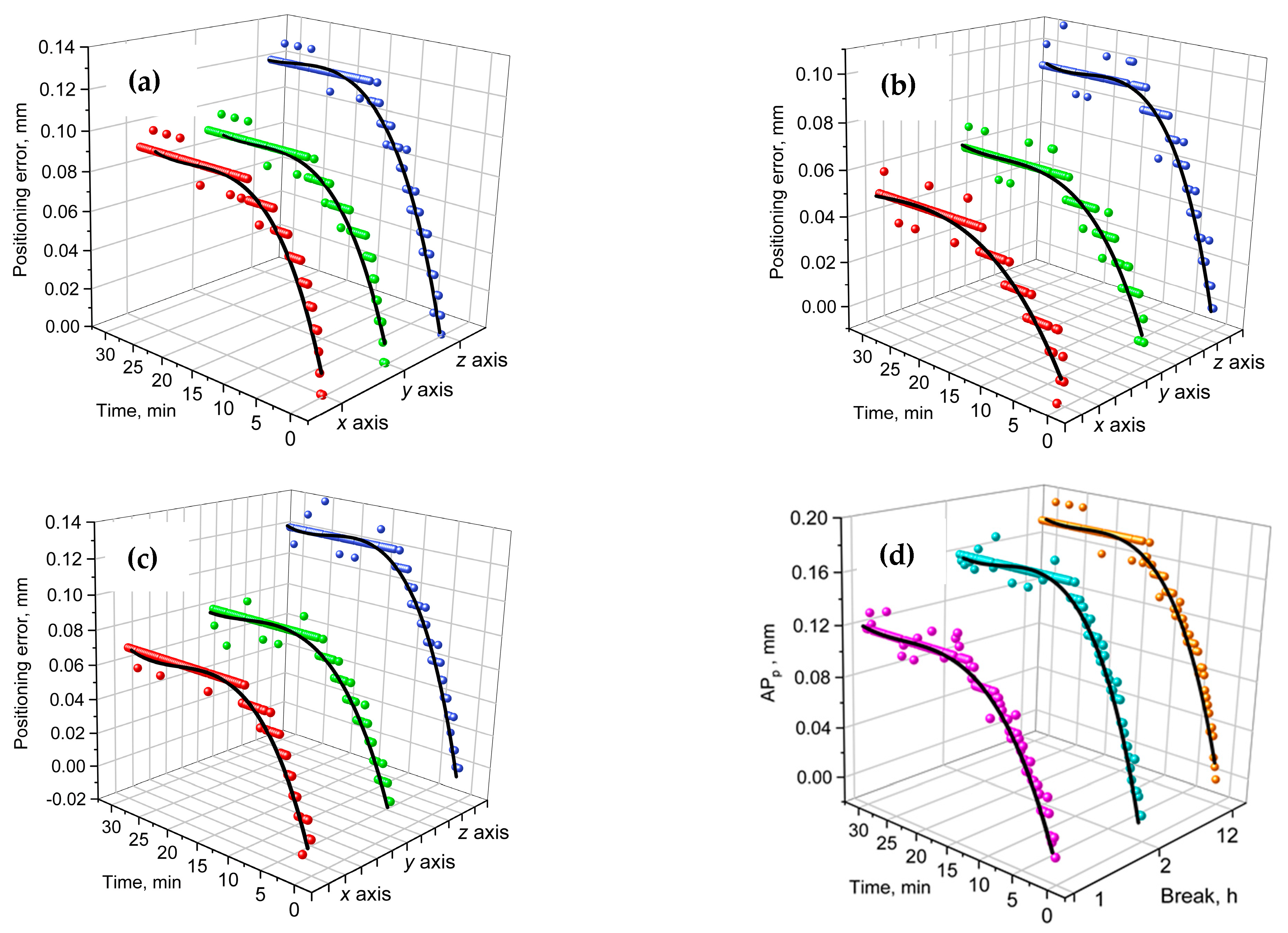
The robot’s accuracy after a long operation break degenerates because of the temperature regime change and lubricant film disappearance from joint clearances. Thus, the measurement of the positioning error of the robot after a long operation break is important for determining the accuracy of restoring to operating time. To determine the robot’s positioning accuracy in time, the positioning error measurement was performed in the x, y, and z-axes when the robot starts to operate after a 12-h break (Figure 8a). In all axes, positioning error increases in the first 14 min of operation time. Positioning errors in the x and y-axes are almost identical as follows: after 14 min, errors are 0.09 mm in both the x and y-axis, while in the z-axis, the error is 0.12 mm.

Regression approximation parameters are provided in

Table 3. Coefficients for the regression estimated robot positioning error.

Operation Break	Axis	a0	a1	a2	a3
1-h	x	2.8464 × 10−4	5.5500 × 10−3	−1.9554 × 10−4	2.1655 × 10−6
	y	1.6700 × 10−3	7.7700 × 10−3	−3.3957 × 10−4	4.9016 × 10−6
	z	−4.6000 × 10−3	1.3590 × 10−2	−6.3174 × 10−4	9.5758 × 10−6
	APp	8.5400 × 10−3	2.2560 × 10−2	−1.0000 × 10−3	1.4723 × 10−5
2-h	x	−7.3200 × 10−3	1.2260 × 10−2	−6.1872 × 10−4	9.9370 × 10−6
	y	−5.8300 × 10−3	1.1690 × 10−2	−5.0854 × 10−4	7.0670 × 10−6
	z	−9.7000 × 10−3	1.8300 × 10−2	−8.2850 × 10−4	1.2126 × 10−6
	APp	−1.1120 × 10−2	2.4470 × 10−2	−1.1200 × 10−3	1.6540 × 10−5
12-h	x	8.0000 × 10−3	1.2340 × 10−2	−6.1009 × 10−4	9.8658 × 10−6
	y	7.5200 × 10−3	1.1750 × 10−2	−5.5304 × 10−4	8.5685 × 10−6
	z	−2.7500 × 10−3	1.5180 × 10−2	−6.0424 × 10−4	7.8195 × 10−6
	APp	4.5125 × 10−4	1.5930 × 10−2	−6.9624 × 10−4	9.9989 × 10−6

.

Results of experiments performed after a 1-h and 12-h operation break showed that the required warm-up period is 14 min (Figure 8b). However, with a 1-h break, positioning errors decreased compared to a 12-h break, causing the following errors: 0.05 mm in the x-axis, 0.06 mm in the y-axis, and 0.09 mm in the z-axis. This phenomenon can be explained by the fact that 1 h is not enough for all joints to cool down to the initial temperature and to sediment the lubricant layer. The uneven distribution of positioning errors in the x and y axes requires an increase in the operational break. To check this assumption, the same experiments were performed after a 2 h break (Figure 8c).

It was observed that the time until positioning errors become stable is 12.5 min for the y and z-axes and 11.2 min for the x-axis. The stable positioning error in the x-axis is 0.07 mm, 0.08 mm in the y-axis, and 0.12 mm in the z-axis. This situation is quite similar to the case when the robot starts operating after a 12-h break. Small differences can be explained by assuming that after a 2-h break, the robot almost cools down, but some elements in separate joints may still have higher temperatures.

From the dependencies between positioning error fluctuations over time, we can define the minimum required warm-up period for the robot or predict the positioning accuracy in respect of operating time. Moreover, the obtained data allow us to define the robot’s overall positioning accuracy and repeatability.

Results presented in Figure 8d correspond to results presented in Figure 8a–c where it is seen that after a lengthy break (12 h), overall positioning precision depends upon time. In the first 13 min of operation after the 1-h break, positioning error slightly increases up to 0.12 mm. After a 2-h break, the error reaches 0.16 mm, and finally 0.17 mm after a 12-h break. This allows us to state that the minimum warm-up time required for the robot to reach stable positioning accuracy values is more than 14 min.

The repeatability error of the robot was specified using experimental data provided in Figure 8d. The overall evaluation of repeatability error after data processing is 0.0146 ± 0.00526 mm (Equations (6) and (7)).

The collected data suggest that, if the robot stays idle for an hour or more, in order to achieve a higher level of accuracy and repeatability, it is recommended that within the first 14 min after the break, do not perform any operational action, but rather use some warm-up programs. In other cases, we can provide coordinates of the prescribed position, which should be adjusted according to the dependencies obtained during this research. The value and direction of defined positioning error become important parameters for compensation used in ML-based robot trajectory correction. The ML process will use the value and direction of the defined positioning error as parameters and use them as the target line for further process of ML. The orientation of the error vector also has meaning for error compensation. In the case of a simulation procedure rather than an experimental ML approach, there is a chance to significantly decrease learning time. Obtained data will have a value not only as an absolute achieved point but also as a beacon for further learning, especially when another loading configuration or load occurs.

We observed the positioning error dependencies over time and after a long operation break. These dependencies can be included in ML algorithms to compensate for positioning errors at different periods of the warming process operating times.

4.2. Definition of Robot Positioning Accuracy

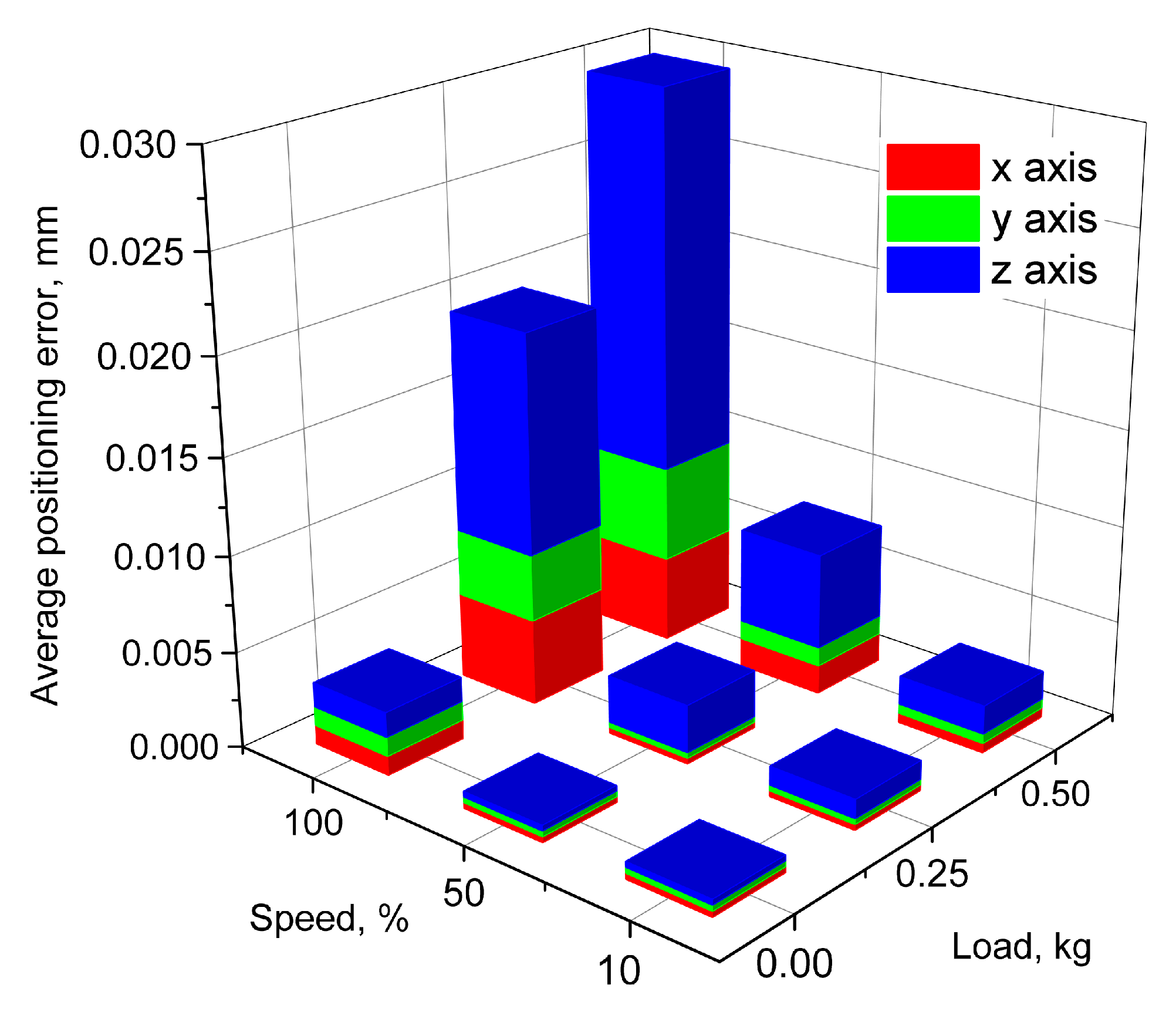
The accuracy of robot positioning was examined when the robot was moved at various speeds with different loads. Positioning errors were measured in the following three perpendicular directions: x, y, and z (Figure 9). The average distribution of positioning errors was calculated using Equation (12) when the robot moves at the speed values of 10%, 50%, and 100% of maximum speed for every joint being unloaded or with 0.25 kg and 0.50 kg loads.

It was defined that in all researched cases, the highest positioning error value appears along the z-axis operating at maximum speed (90°/s). When the robot moves in unloaded mode, the average positioning error in the z-axis is 0.0014 mm. When the robot moves with a 0.50 kg load, this error increases up to 0.02 mm. A similar tendency is noticed when analyzing the accuracy of the x and y-axis, but in those cases, when the values of positioning errors are lower compared with values of the z-axis as follows: 0.001 mm when the robot moves unloaded and 0.005 mm when the robot moves with a 0.50 kg load.

The results of the measurements allow us to state that if the robot is warmed up, positioning accuracy of ±0.03 mm can be achieved with a maximum (0.50 kg) weight at the highest speed (90°/s). At lower loads or at lower speeds, it is possible to achieve a positioning accuracy of up to ±0.01 mm (Figure 9).

Results obtained from accuracy and repeatability measurements show that at desired conditions, the robot achieves better parameters compared to the ones declared by the manufacturer [39]. The achieved values of positioning error with prescribed load and speed let us compensate key-point coordinates through ML procedure and achieve actual positioning accuracy higher than guaranteed by the robot producer.

Moreover, ML can compensate for the dynamic error of the robot, but for this purpose, it is necessary to analyze the actual vibrations during the robot’s movement. Measurements of robot vibrations allow us to fulfill information about positioning accuracy by evaluating such parameters as maximum vibration level and settling time when the robot stops at the desired position. The results of these researches are presented in the next subchapter. The error values are derived from experimental research as error ranges, and the direction of error known as well; therefore, the compensation is performed in advance for defined load and robot configuration.

4.3. Measurement of the Robot Vibrations

Data obtained from robot vibration measurements allowed us to define the average vibration level of the end-of-arm reference point and settling time. These characteristics describe the robot’s dynamics and have a great influence on its accuracy and operating speed. In addition, these characteristics allow indirect evaluation of position overshoots and show the minimum required time to reach a stable position after movement. This is extremely important in robotics for the assembly of precise objects and the cooperation of several robots.

Statistically evaluated results show the average level of the reference point absolute vibration acceleration values (Figure 10).

From Figure 10a, it is seen that the average amplitude of the vibrations increases when the speed of the robot increases practically on all measured axes. The highest values of vibration levels were recorded at the highest speed. Comparing vibration levels in separate axes, we noticed that the highest values (0.75 g at speed 10% and 1.6 g at speed 100%) were defined on the y-axis.

Results presented in Figure 10b show the following inverse tendency: here, the highest values of vibration level occur when the robot moves at 10% speed. By analyzing the vibration level in the z-axis direction, it was 0.87 g at 10% speed, 0.6 g at 50% speed, and 0.75 g at 100% speed. A similar tendency was also defined by analyzing the x and y-axes.

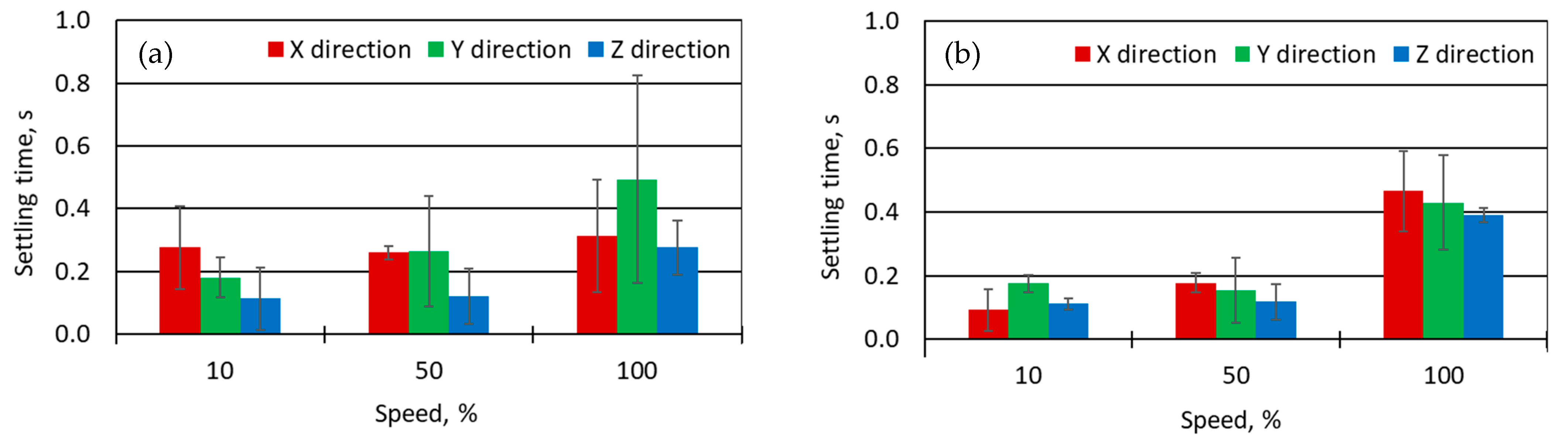
Controversial results regarding Figure 10a,b can be explained by the fact that when the robot moves up from the start position, the gravitational force acts as an additional load; when the robot moves down from the endpoint of the trajectory, gravity acts in the same direction as robot displacement (Figure 2). This analysis was useful to evaluate the settling time of vibrations (Figure 11).

Settling time for all axes increases with movement speed; however, the resulting settling time of the x-axis at 50% speed does not follow this tendency (Figure 11a). At the ends of the trajectory (Figure 3), the lowest defined settling time is 0.1 s, whilst the highest value is equal to 0.5 s. Comparing the results presented in Figure 11a,b, the impact of the direction of gravity on the direction of the robot’s movement is demonstrated. Settling time in the case when the robot moves from its starting point is about 0.07 s. If the robot moves from its trajectory endpoint, it does not exceed 0.2 s. Results presented in Figure 10 and Figure 11 allow us to state that the vibration level when the robot stops depends not only on the movement speed but also on the movement direction. The results of all experimental research revealed the settling time did not exceed 0.5 s.

4.4. Separate Joint Vibrations Evaluation

To evaluate the behavior of each joint, we performed a separate experiment, which allows defining the influence of each joint on the general vibrations of the entire robot (Figure 12).

Peak-to-peak vibration amplitudes were evaluated after the rotation of separate joints (Figure 4). The largest measured vibration amplitude was recorded at the x and y axes. The largest amplitude of all measurements was recorded when rotating joint II in a clockwise direction (0.6 g), and the smallest amplitude was recorded when rotating joint V (in a counterclockwise direction, 0.05 g). Probably some variations in clockwise and counterclockwise directions were produced by gravity, which was affecting the robot’s movement. Results of measured settling time when separate joints were moved are presented in Figure 13.

From Figure 13a, it is seen that settling time had the greatest value in the x and y directions when joint II was rotated. When the robot joints move clockwise (Figure 13b), the longest settling time was recorded when rotating the second and third joints. The shortest settling time was detected while moving joint I and joint V in both cases. Results obtained from this experiment show that dynamic robot characteristics are mostly affected by the characteristics of the second and third joints, and the settling time at various positions can be more than 0.5 s.

4.5. Extended Position Vibration Measurement

The impact of the first joint characteristics on the robot vibrations when this joint is loaded by maximum force due to an extended robot arm was evaluated (Figure 5). Under such conditions, the maximum vibration level is expected to be influenced by the gravity force direction.

From Figure 14, the highest level of vibration, 0.46 g, was detected in the x-axis when the robot is at an extended position; in the compact position case, this value was 0.27 g. The lower levels of vibrations were detected in the y and z-axes. The moderately high level of vibrations in the z-axis allows us to state that during the movement of the first joint, the whole structure of the robot is kinematically excited. In the extended position, the longest settling time of 0.56 s was defined in the z-axis, while in the compact position, the longest settling time of 0.44 s was detected in the y-axis. This can be explained by the fact that in various configurations, due to the distribution of mass centers, the variable loads and inertia forces in all joints can be detected. Thus, it could be concluded that in most uncomfortable configurations, settling time will not exceed 0.6 s.

4.6. Experiment with Implemented Correction

The correction was applied to the real (Kuka YouBot) robot using processed experimental data. The flowchart of the performed procedure is presented in Figure 15. During the first run, algorithms take experimentally defined data representing robot characteristics and previous compensation values as input parameters and provide an output as a natural number that is later transformed into a new compensation value.

The compensation parameters were applied by shifting the stated start and endpoint positions of the trajectory provided in Figure 3. The efficiency of the proposed methodology was evaluated by measuring positioning accuracy at the start and endpoint of the robot trajectory (Figure 16). During the experiment, the robot was loaded with a 0.5 kg payload and moved at maximum velocity.

The machine learning process was terminated after 780 iterations by the program because the general positioning error stops to decrease. The ML process has different progress for overall positioning error in the start (Figure 3a) and endpoints (Figure 3b) of the trajectory. The learning process at the start point of the trajectory progresses at the 180th iteration, while the process at the endpoint of the trajectory starts approaching the learning target at the 180th iteration and ends at the 240th iteration. Differences in the learning process are influenced by the gravity force depending on the robot links’ configuration.

From the obtained results, we defined the following: the overall positioning error at the start point decreases by 40%: from 0.021 mm to 0.0125 mm; the overall positioning error at the endpoint decreases by 34%: from 0.028 mm to 0.0185 mm.

The proposed method deals with the complex improvement of robot accuracy in comparison with classic methods. Comparison of the proposed method to the existing classic ML methodologies has some scale problems. The online ML process, as proposed in the paper, can minimize robot positioning errors at the interesting point by compensating them in the operation online. Available offline learning procedures are focused on preparatory modes of robot’s implementation. Offline methods, as well as statistical ones (workspace mapping), are not sensitive to the fluctuations of the robot operating process. In such a case, robot installation in the production enterprise begs for readjusting for the time being, while the proposed procedure is valid for active robot operation. The complexity of the evaluated and compensated errors is hidden behind the process—we achieve a goal as a diminishing of robot error regardless of the actual coordinate position and configuration of the robot in the target point position. The distribution of the task components along the axes as it is performed for some methods here is not applicable. The disadvantage of the proposed method is some operational time for the ML procedure to set up compensation values, so actual disturbances of the robotic system can cause some periods of increased error values. The good point of the proposed method—initial data collection is possible to optimize. There are available synthetic (simulated) data implementations into the learning process and the use of advanced technical equipment for automated data collection.

5. Conclusions

The dynamic behavior of a robot is to a large extent affected by the robot’s warming-up time, the load, the speed of movement, and the trajectory in the working space. The experimental research on warming-up time showed that the highest positioning error was 0.12 mm if the robot operated without warm-up. The optimal time for warming up is 14–15 min. The completed research allowed a conclusion that when the manipulator stays idle for 1 h or more, it is recommended to allow the manipulator to operate initially without performing any work. Where the use of a warm-up program is inconvenient, higher positioning accuracy can be achieved by adjusting the prescribed positions according to experimentally defined dependencies between positioning errors and operating time. Implementing ML here could compensate for positioning errors during the robot warming period if the learning procedure can be taken for many operation breaks. Robot repeatability measured after the warming-up process was 0.0146 ± 0.00526 mm.

Research performed when the robot moves at various speeds with various loads showed that the highest 0.019 mm positioning error appeared in the z-axis when the robot moves at its highest speed with a 0.50 kg load. The obtained results significantly exceed the tolerance of ±1.0 mm declared by the manufacturer. This allows us to state that ML can improve the accuracy of industrial robots with known operating and environmental conditions. ML is suitable for positioning static and dynamic error compensation for steady-state trajectory and fast accuracy improvement during initial or test operation. The obtained accuracy error value is better than that declared by the manufacturer, and it can even be improved for precision operations; the manufacturer could also implement this option using ML procedures.

Results obtained from vibration measurements show that gripper vibration amplitude mostly depends on the movement trajectory, speed, and direction; the highest measured peak-to-peak vibration amplitude, 1.6 g, was observed at maximum (90°/s) speed. Additional research performed with separate joints showed that the highest impact on the overall vibration level is on joint II and joint III if the robot operates in common configurations. When the robot operates in the closed position, overall vibration levels are mostly affected by joint I.

The results of the settling time measurements, in most cases, correspond to the results of vibration measurements. It was noticed that settling time in most of the tests depends on movement speed, while vibration amplitude is additionally affected by movement direction. The longest settling time was defined as 0.55 s at maximum speed. Therefore, this allows us to state that when operating at maximum speed, the settling time for the robot can last up to 0.6 s.

The set of results obtained from our research allows us to predict the behavior of the analyzed robot and to define its characteristics under various conditions. These results can be used to improve robot parameters for precise operations. Moreover, this result and methodology can be used as a basic database for creating and implementing in practice various ML algorithms. To compensate for positioning errors, the data about the current robot operation must be collected and processed in a way suitable to further use in ML. First, positioning accuracy and vibrations under various conditions in positions that are important for the performing task and in which the accuracy is diminished (for example, near the singularity) should be determined experimentally. Second, the measurements of vibrations on the end-of-arm reference point, including measurements of separate joint impact to general vibration level, should be performed. Then the collected data can be processed using ML algorithms.