

Image-Processing-Based Intelligent Defect Diagnosis of Rolling Element Bearings Using Spectrogram Images


Abstract
:1. Introduction
2. Theoretical Background
2.1. Spectrogram
2.2. Artificial Neural Network
2.3. K-Nearest Neighbors
2.4. Support Vector Machine
2.5. Convolutional Neural Network
Transfer Learning
2.6. Image Features Extraction
2.6.1. Deep Features
2.6.2. Handcrafted Features
Histogram of Oriented Gradient
Local Binary Patterns
3. Experimental Setup and Vibration Data
4. Applied Methodology
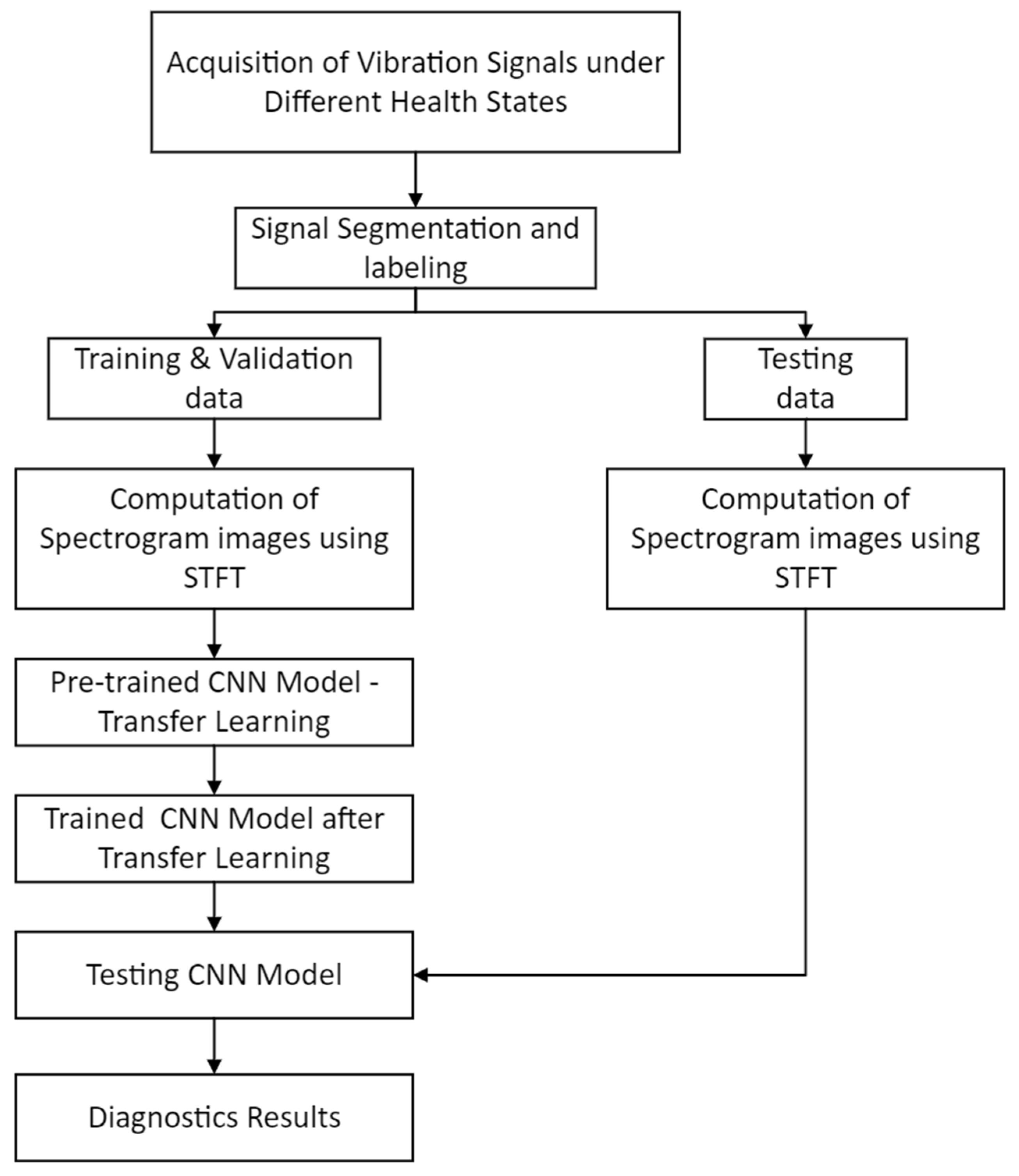
4.1. Method-1 (CNN as End-to-End Classifier—Transfer Learning)
4.2. Method-II (Deep Features + Classical ML Models)
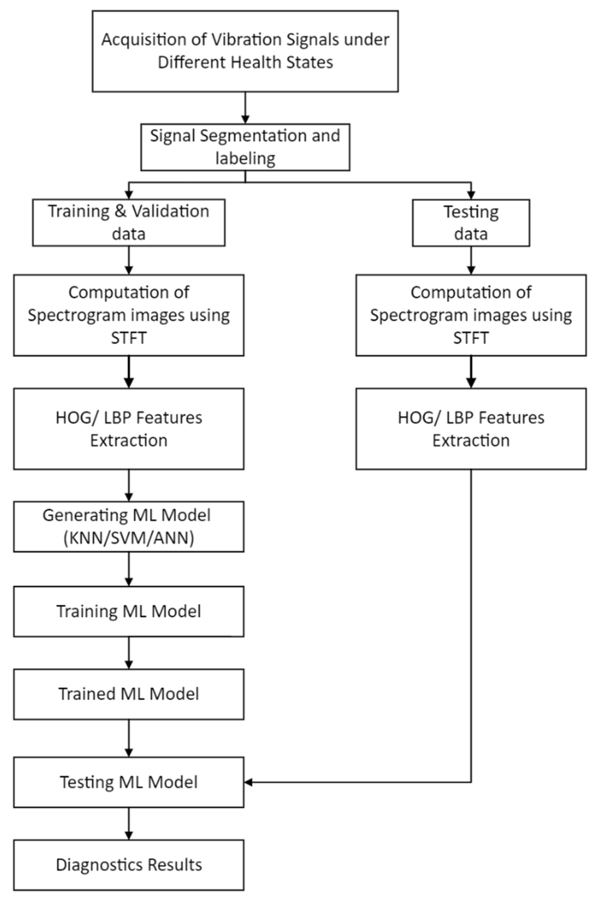
4.3. Method-III (Handcrafted Features + ML Model)
4.4. Proposed Hybrid-Ensemble Method
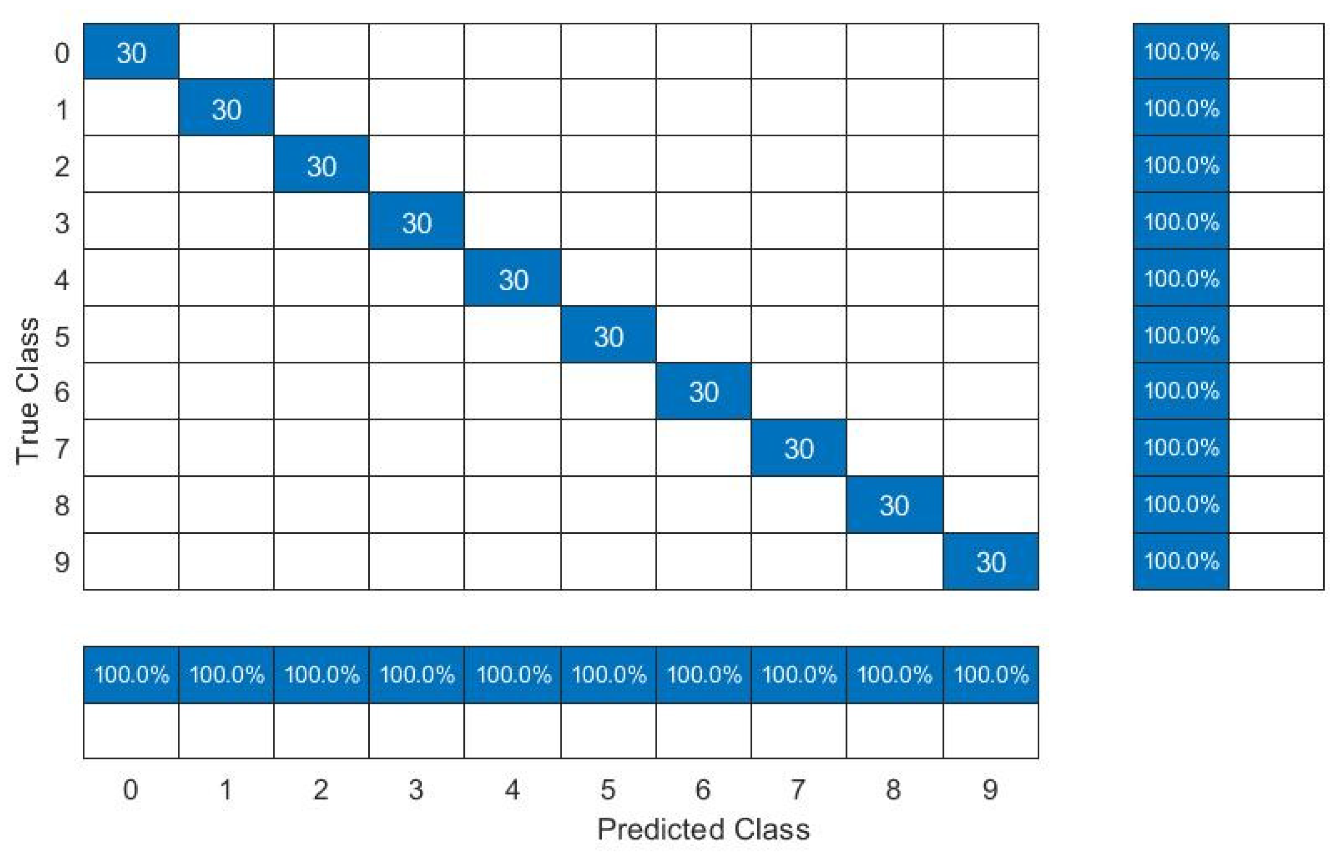
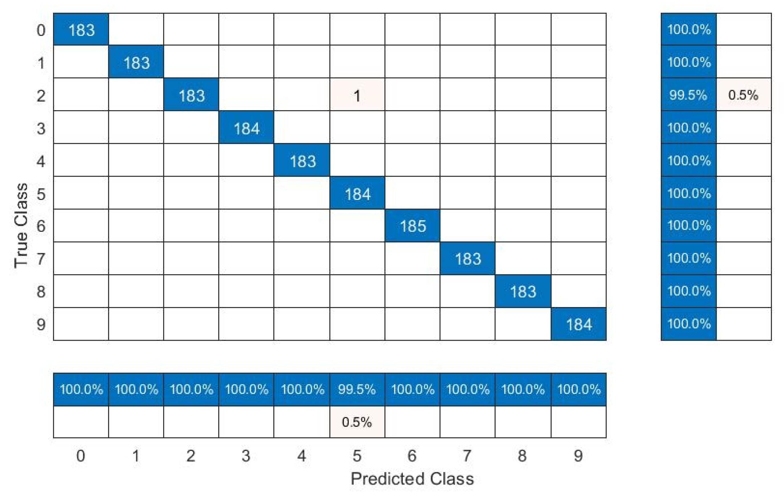
5. Results and Discussion
6. Conclusions
Author Contributions
Funding
Institutional Review Board Statement
Informed Consent Statement
Data Availability Statement
Conflicts of Interest
References
- Kiral, Z.; Karagülle, H. Simulation and analysis of vibration signals generated by rolling element bearing with defects. Tribol. Int. 2003, 36, 667–678. [Google Scholar] [CrossRef]
- Orhan, S.; Aktürk, N.; Çelik, V. Vibration monitoring for defect diagnosis of rolling element bearings as a predictive maintenance tool: Comprehensive case studies. Ndt E Int. 2006, 39, 293–298. [Google Scholar] [CrossRef]
- Li, B.; Chow, M.Y.; Tipsuwan, Y.; Hung, J. Neural-network-based motor rolling bearing fault diagnosis. IEEE Trans. Ind. Electron. 2000, 47, 1060–1069. [Google Scholar] [CrossRef] [Green Version]
- Samanta, B.; Al-Balushi, K.R. Artificial neural network based fault diagnostics of rolling element bearings using time-domain features. Mech. Syst. Signal Process. 2003, 17, 317–328. [Google Scholar] [CrossRef]
- Tayyab, S.M.; Asghar, E.; Pennacchi, P.; Chatterton, S. Intelligent fault diagnosis of rotating machine elements using machine learning through optimal features extraction and selection. Procedia Manuf. 2020, 72, 266–273. [Google Scholar] [CrossRef]
- Seryasat, O.R.; Haddadnia, J.; Arabnia, Y.; Zeinali, M.; Abooalizadeh, Z.; Taherkhani, A.; Tabrizy, S.; Maleki, F. Intelligent fault detection of ball-bearings using artificial neural networks and support-vector machine. Life Sci. 2012, 9, 4186–4189. [Google Scholar]
- Mao, W.; He, J.; Li, Y.; Yan, Y.G. Bearing fault diagnosis with auto-encoder extreme learning machine: A comparative study. Proc. Inst. Mech. Eng. C J. Mech. Eng. Sci. 2017, 231, 1560–1578. [Google Scholar] [CrossRef]
- Su, H.; Chong, K.T. Induction machine condition monitoring using neural network modeling. IEEE Trans. Ind. Electron. 2007, 54, 241–249. [Google Scholar] [CrossRef]
- Wu, C.X.; Chen, T.F.; Jiang, R. Bearing fault diagnosis via kernel matrix construction based support vector machine. J. Vibroengineering 2017, 19, 3445–3461. [Google Scholar] [CrossRef] [Green Version]
- Gunerkar, R.S.; Jalan, A.K.; Belgamwar, S.U. Fault diagnosis of rolling element bearing based on artificial neural network. J. Mech. Sci. Technol. 2019, 33, 505–511. [Google Scholar] [CrossRef]
- Patel, J.P.; Upadhyay, S.H. Comparison between artificial neural network and support vector method for a fault diagnostics in rolling element bearings. Procedia Eng. 2016, 144, 390–397. [Google Scholar] [CrossRef]
- Hussain, M.; Bird, J.J.; Faria, D.R. A Study on CNN Transfer Learning for Image Classification. In Advances in Computational Intelligence Systems; Springer: Cham, Switzerland, 2019; pp. 191–202. [Google Scholar] [CrossRef]
- Eren, L. Bearing fault detection by one-dimensional convolutional neural networks. Math. Probl. Eng. 2017, 2017, 8617315. [Google Scholar] [CrossRef] [Green Version]
- Eren, L.; Ince, T.; Kiranyaz, S. A generic intelligent bearing fault diagnosis system using compact adaptive 1D CNN classifier. J. Signal Process. Syst. 2019, 91, 179–189. [Google Scholar] [CrossRef]
- Pham, M.-T.; Kim, J.-M.; Kim, C.-H. 2D CNN-Based Multi-Output Diagnosis for Compound Bearing Faults under Variable Rotational Speeds. Machines 2021, 9, 199. [Google Scholar] [CrossRef]
- Pham, M.-T.; Kim, J.-M.; Kim, C.-H. Accurate bearing fault diagnosis under variable shaft speed using convolutional neural networks and vibration spectrogram. Appl. Sci. 2020, 10, 6385. [Google Scholar] [CrossRef]
- Verstraete, D.; Ferrada, A.; Droguett, E.L.; Meruane, V.; Modarres, M. Deep learning enabled fault diagnosis using time-frequency image analysis of rolling element bearings. Shock. Vib. 2017, 2017, 5067651. [Google Scholar] [CrossRef] [Green Version]
- Tang, H.D.; Tran, X.T.; Van, M.; Kang, H.J. A Deep Neural Network-Based Feature Fusion for Bearing Fault Diagnosis. Sensors 2021, 21, 244. [Google Scholar] [CrossRef]
- Tayyab, S.M.; Chatterton, S.; Pennacchi, P. Intelligent Defect Diagnosis of Rolling Element Bearings under Variable Operating Conditions Using Convolutional Neural Network and Order Maps. Sensors 2022, 22, 2026. [Google Scholar] [CrossRef]
- Hoang, D.-T.; Kang, H.-J. Rolling element bearing fault diagnosis using convolutional neural network and vibration image. Cogn. Syst. Res. 2019, 53, 42–50. [Google Scholar] [CrossRef]
- Deng, J.; Dong, W.; Socher, R.; Li, L.-J.; Li, K.; Li, F.-F. ImageNet: A large-scale hierarchical image database. In Proceedings of the 2009 IEEE Conference on Computer Vision and Pattern Recognition, Miami, FL, USA, 20–25 June 2009; pp. 248–255. [Google Scholar] [CrossRef]
- Russakovsky, O.; Deng, J.; Su, H.; Krause, J.; Satheesh, S.; Ma, S.; Huang, Z.; Karpathy, A.; Khosla, A.; Bernstein, M.; et al. ImageNet Large Scale Visual Recognition Challenge. Int. J. Comput. Vis. 2015, 115, 211–252. [Google Scholar] [CrossRef] [Green Version]
- Bai, Y.; Yang, J.; Wang, J.; Zhao, Y.; Li, Q. Image representation of vibration signals and its application in intelligent compound fault diagnosis in railway vehicle wheelset-axlebox assemblies. Mech. Syst. Signal Process. 2021, 152, 107421. [Google Scholar] [CrossRef]
- Yosinski, J.; Clune, J.; Bengio, Y.; Lipson, H. How transferable are features in deep neural networks? Adv. Neural Inf. Process. Syst. 2014, 27, 1–9. [Google Scholar]
- Udmale, S.S.; Singh, S.K.; Singh, R.; Sangaiah, A.K. Multi-fault bearing classification using sensors and ConvNet-based transfer learning approach. IEEE Sens. J. 2019, 20, 1433–1444. [Google Scholar] [CrossRef]
- Xie, W.; Li, Z.; Xu, Y.; Gardoni, P.; Li, W. Evaluation of Different Bearing Fault Classifiers in Utilizing CNN Feature Extraction Ability. Sensors 2022, 22, 3314. [Google Scholar] [CrossRef]
- Khan, S.A.; Kim, J.M. Automated bearing fault diagnosis using 2D analysis of vibration acceleration signals under variable speed conditions. Shock. Vib. 2016, 2016, 8729572. [Google Scholar] [CrossRef] [Green Version]
- Kaplan, K.; Kaya, Y.; Kuncan, M.; Minaz, M.R.; Ertunç, H.M. An improved feature extraction method using texture analysis with LBP for bearing fault diagnosis. Appl. Soft Comput. 2020, 87, 106019. [Google Scholar] [CrossRef]
- Chen, J.; Zhou, D.; Wang, Y.; Fu, H.; Wang, M. Image feature extraction based on HOG and its application to fault diagnosis for rotating machinery. J. Intell. Fuzzy Syst. 2018, 34, 3403–3412. [Google Scholar] [CrossRef]
- Tayyab, S.M.; Chatterton, S.; Pennacchi, P. Fault detection and severity level identification of spiral bevel gears under different operating conditions using artificial intelligence techniques. Machines 2021, 9, 173. [Google Scholar] [CrossRef]
- Er-Raoudi, M.; Diany, M.; Aissaoui, H.; Mabrouki, M. Gear fault detection using artificial neural networks with discrete wavelet transform and principal component analysis. J. Mech. Eng. Sci. 2016, 10, 2016–2029. [Google Scholar] [CrossRef]
- Yang, D.M.; Stronach, A.F.; MacConnell, P.; Penman, J. Third-order spectral techniques for the diagnosis of motor bearing condition using artificial neural networks. Mech. Syst. Signal Process. 2002, 16, 391–411. [Google Scholar] [CrossRef]
- Liu, R.; Yang, B.; Zio, E.; Chen, X. Artificial intelligence for fault diagnosis of rotating machinery: A review. Mech. Syst. Signal Process. 2018, 108, 33–47. [Google Scholar] [CrossRef]
- Baraldi, P.; Cannarile, F.; Di Maio, F.; Zio, E. Hierarchical k-nearest neighbours classification and binary differential evolution for fault diagnostics of automotive bearings operating under variable conditions. Eng. Appl. Artif. Intell. 2016, 56, 1–13. [Google Scholar] [CrossRef] [Green Version]
- Lei, Y.G.; Yang, B.; Jiang, X.W.; Feng, J.; Li, N.P.; Asoke, K.N. Applications of machine learning to machine fault diagnosis: A review and roadmap. Mech. Syst. Signal Process. 2019, 138, 106587. [Google Scholar] [CrossRef]
- Dalal, N.; Triggs, B. Histograms of oriented gradients for human detection. In Proceedings of the in 2005 IEEE Computer Society Conference on Computer Vision and Pattern Recognition (CVPR’05), San Diego, CA, USA, 20–25 June 2005; Volume 1, pp. 886–893. [Google Scholar] [CrossRef] [Green Version]
- Kumar, M.D.; Babaie, M.; Zhu, S.; Kalra, S.; Tizhoosh, H.R. A comparative study of CNN, BoVW and LBP for classification of histopathological images. In Proceedings of the2017 IEEE Symposium Series on Computational Intelligence (SSCI), Honolulu, HI, USA, 27 November 2017–1 December 2017; IEEE: Piscataway, NJ, USA, 2017. [Google Scholar] [CrossRef] [Green Version]
- Case Western Reserve University Bearing Data Center. Available online: https://engineering.case.edu/bearingdatacenter/download-data-file (accessed on 25 April 2022).
- Krizhevsky, A.; Sutskever, I.; Hinton, G.E. ImageNet Classification with Deep Convolutional Neural Networks. Adv. Neural Inf. Process. Syst. 2012, 60, 84–90. [Google Scholar] [CrossRef] [Green Version]
- Iandola, F.N.; Han, S.; Moskewicz, M.W.; Ashraf, K.; Dally, W.J.; Keutzer, K. SqueezeNet: AlexNet-level accuracy with 50x fewer parameters and <0.5 MB model size. arXiv 2016, arXiv:1602.07360. [Google Scholar] [CrossRef]
- Szegedy, C.; Liu, W.; Jia, Y.; Sermanet, P.; Reed, S.; Anguelov, D.; Erhan, D.; Vanhoucke, V.; Rabinovich, A. Going deeper with convolutions. In Proceedings of the IEEE Conference on Computer Vision and Pattern Recognition, Boston, MA, USA, 7–12 June 2015; pp. 1–9. [Google Scholar] [CrossRef] [Green Version]
- He, K.; Zhang, X.; Ren, S.; Sun, J. Deep residual learning for image recognition. In Proceedings of the IEEE Conference on Computer Vision and Pattern Recognition, Las Vegas, NV, USA, 26–30 June 2016; pp. 770–778. [Google Scholar] [CrossRef]
- Sandler, M.; Howard, A.; Zhu, M.; Zhmoginov, A.; Chen, L.-C. Mobilenetv2: Inverted residuals and linear bottlenecks. In Proceedings of the IEEE Conference on Computer Vision and Pattern Recognition 2018, Salt Lake City, UT, USA, 18–23 June 2018; pp. 4510–4520. [Google Scholar] [CrossRef]
- Szegedy, C.; Vanhoucke, V.; Ioffe, S.; Shlens, J.; Wojna, Z. Rethinking the inception architecture for computer vision. In Proceedings of the IEEE Conference on Computer Vision and Pattern Recognition 2016, Las Vegas, NV, USA, 26–30 June 2016; pp. 2818–2826. [Google Scholar] [CrossRef]
- Huang, G.; Liu, Z.; van der Maaten, L.; Weinberger, K.Q. Densely connected convolutional networks. In Proceedings of the IEEE Conference on Computer Vision and Pattern Recognition 2017, Honolulu, HI, USA, 21–26 July 2017; pp. 4700–4708. [Google Scholar] [CrossRef]
- Karen, S.; Zisserman, A. Very deep convolutional networks for large-scale image recognition. arXiv 2014, arXiv:1409.1556. [Google Scholar] [CrossRef]


| Operating Condition (OC) Number | Load (HP) | Speed (rpm—Approximate) |
|---|---|---|
| 1 | 0 | 1797 |
| 2 | 1 | 1772 |
| 3 | 2 | 1749 |
| 4 | 3 | 1720 |
| S. No | Defect Class Number | Defect Type | Defect Size (Inches) |
|---|---|---|---|
| 1 | 0 | Normal/healthy | - |
| 2 | 1 | Ball defect | 0.007 |
| 3 | 2 | Ball defect | 0.014 |
| 4 | 3 | Ball defect | 0.021 |
| 5 | 4 | Inner race defect | 0.007 |
| 6 | 5 | Inner race defect | 0.014 |
| 7 | 6 | Inner race defect | 0.021 |
| 8 | 7 | Outer race defect | 0.007 |
| 9 | 8 | Outer race defect | 0.014 |
| 10 | 9 | Outer race defect | 0.021 |
| S. No | Network/Model | Input Image Size |
|---|---|---|
| 1 | AlexNet [39] | 227-by-227 |
| 2 | SqueezeNet [40] | 227-by-227 |
| 3 | GoogLeNet [41] | 224-by-224 |
| 4 | ResNet-18 [42] | 224-by-224 |
| 5 | MobileNet-v2 [43] | 224-by-224 |
| 6 | Inception-v3 [44] | 299-by-299 |
| 7 | DenseNet-201 [45] | 224-by-224 |
| 8 | ResNet-50 [42] | 224-by-224 |
| 9 | ResNet-101 [42] | 224-by-224 |
| 10 | VGG -16 [46] | 224-by-224 |
| 11 | VGG -19 [46] | 224-by-224 |
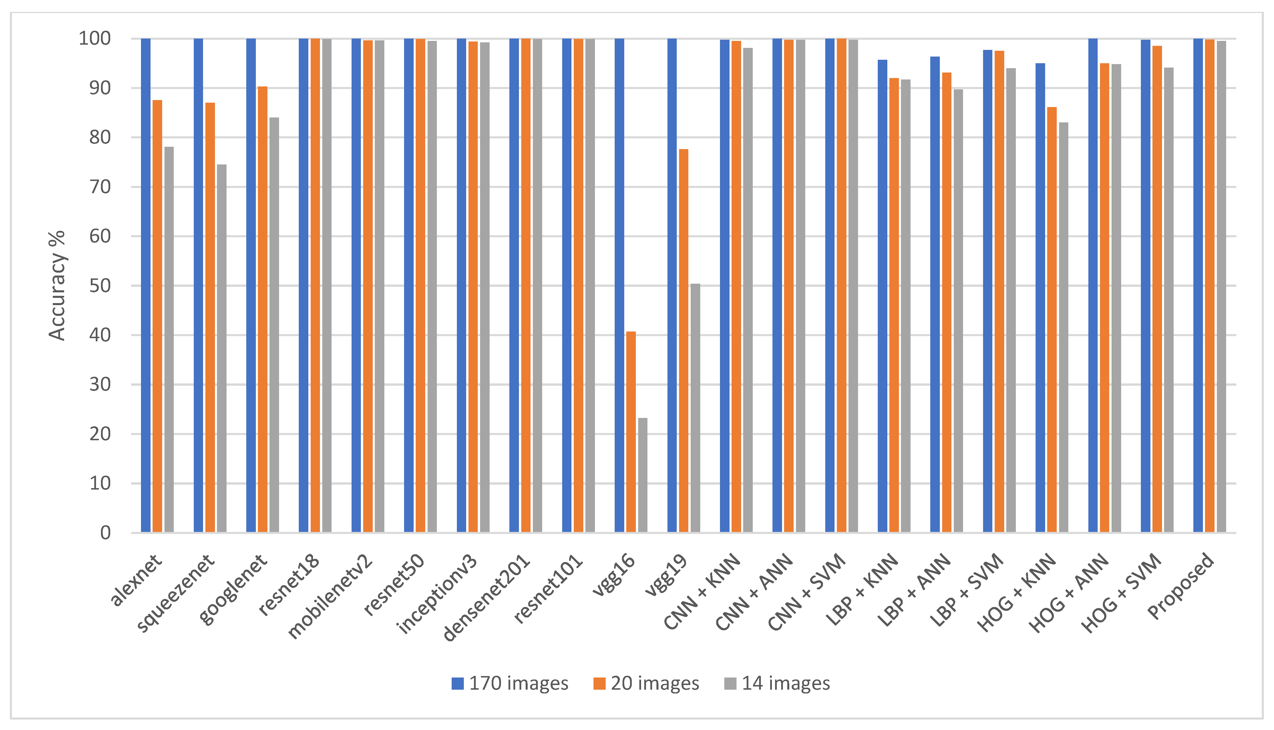
| Size of Training Dataset (for Each Class) | 170 Images | 20 Images | 14 Images | ||||
|---|---|---|---|---|---|---|---|
| Method | Accuracy (%) | Time (s) | Relative Time with Respect to AlexNet | Accuracy (%) | Accuracy (%) | ||
| 1 | Transfer learning from pretrained CNN models on ImageNet dataset | AlexNet | 100 | 1026.1 | 1 | 87.5 | 78.1 |
| SqueezeNet | 100 | 1206.4 | 1.2 | 87 | 74.5 | ||
| GoogLeNet | 100 | 1817.9 | 1.8 | 90.3 | 84 | ||
| ResNet-18 | 100 | 1849.8 | 1.8 | 100 | 99.9 | ||
| MobileNet-v2 | 100 | 3053.1 | 2.9 | 99.6 | 99.6 | ||
| ResNet-50 | 100 | 4772.4 | 4.6 | 99.9 | 99.5 | ||
| Inception-v3 | 100 | 6347.5 | 6.2 | 99.4 | 99.2 | ||
| DenseNet-201 | 100 | 9655.8 | 9.4 | 100 | 99.9 | ||
| ResNet-101 | 100 | 7691.9 | 7.5 | 99.9 | 99.9 | ||
| VGG -16 | 100 | 8632.2 | 8.4 | 40.7 | 23.2 | ||
| VGG -19 | 100 | 12,875.5 | 12.6 | 77.6 | 50.4 | ||
| 2 | Deep CNN features + ML model | CNN + KNN | 99.7 | 117.5 | 0.11 | 99.5 | 98.1 |
| CNN + ANN | 100 | 205.4 | 0.2 | 99.7 | 99.7 | ||
| CNN + SVM | 100 | 118.03 | 0.12 | 100 | 99.7 | ||
| 3 | Handcrafted features + ML model | LBP + KNN | 95.7 | 53.2 | 0.08 | 92 | 91.7 |
| LBP + ANN | 96.3 | 60 | 0.07 | 93.1 | 89.7 | ||
| LBP + SVM | 97.7 | 58.99 | 0.08 | 97.5 | 94 | ||
| HOG + KNN | 95 | 195.5 | 0.2 | 86.1 | 83 | ||
| HOG + ANN | 100 | 221.5 | 0.22 | 95 | 94.8 | ||
| HOG + SVM | 99.7 | 231.6 | 0.27 | 98.5 | 94.1 | ||
| 4 | Proposed hybrid-ensemble meth. | HOG and deep CNN features + ANN and SVM | 100 | 367 | 0.36 | 99.8 | 99.5 |
| Testing Operating Condition | OC-1 | OC-2 | OC-4 | Average Accuracy (%) | ||
|---|---|---|---|---|---|---|
| Method | Accuracy (%) | Accuracy (%) | Accuracy (%) | |||
| 1 | Transfer learning from pretrained CNN models on ImageNet dataset | AlexNet | 96.5 | 87.5 | 95 | 93 |
| SqueezeNet | 92.8 | 89.7 | 96.8 | 93.1 | ||
| GoogLeNet | 91.7 | 89.7 | 98.6 | 93.3 | ||
| ResNet-18 | 98.5 | 89.7 | 90.6 | 92.9 | ||
| MobileNet-v2 | 96.6 | 88.9 | 94.1 | 93.2 | ||
| ResNet-50 | 96.9 | 89 | 93.5 | 93.1 | ||
| Inception-v3 | 96.2 | 87.7 | 90 | 91.3 | ||
| DenseNet-201 | 95.7 | 89.4 | 92.1 | 92.4 | ||
| ResNet-101 | 98.8 | 89.6 | 94.6 | 94.3 | ||
| VGG-16 | 83.9 | 89.5 | 88.5 | 87.3 | ||
| VGG-19 | 87.2 | 89.4 | 97.9 | 91.5 | ||
| 2 | Deep CNN features + ML model | CNN + KNN | 87.8 | 86.8 | 89.1 | 87.9 |
| CNN + ANN | 88.3 | 88.1 | 89.7 | 88.7 | ||
| CNN + SVM | 96.4 | 87.7 | 89.3 | 91.1 | ||
| 3 | Handcrafted features + ML model | LBP + KNN | 32 | 30.7 | 44.2 | 35.6 |
| LBP + ANN | 48.5 | 40.9 | 44.4 | 44.6 | ||
| LBP + SVM | 45.1 | 35.9 | 35.2 | 38.7 | ||
| HOG + KNN | 72 | 66.1 | 72.9 | 70.3 | ||
| HOG + ANN | 92.4 | 88.3 | 97.8 | 92.8 | ||
| HOG + SVM | 80.4 | 73.8 | 87.9 | 80.7 | ||
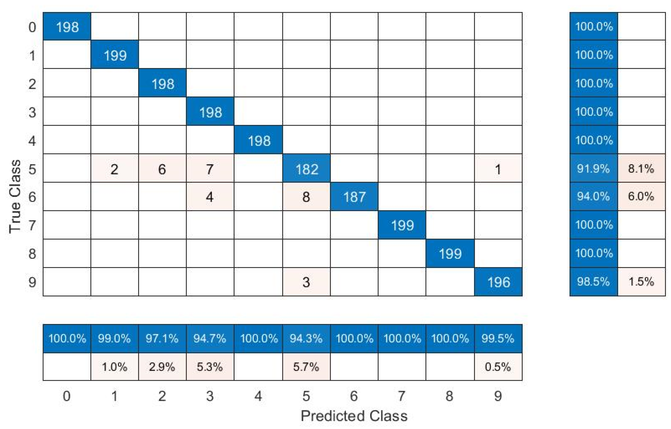
| 4 | Proposed hybrid-ensemble technique | HOG and deep CNN features + ANN and SVM | 99.2 | 89.6 | 98.4 | 95.7 |
Publisher’s Note: MDPI stays neutral with regard to jurisdictional claims in published maps and institutional affiliations. |
© 2022 by the authors. Licensee MDPI, Basel, Switzerland. This article is an open access article distributed under the terms and conditions of the Creative Commons Attribution (CC BY) license (https://creativecommons.org/licenses/by/4.0/).
Share and Cite
Tayyab, S.M.; Chatterton, S.; Pennacchi, P. Image-Processing-Based Intelligent Defect Diagnosis of Rolling Element Bearings Using Spectrogram Images. Machines 2022, 10, 908. https://doi.org/10.3390/machines10100908
Tayyab SM, Chatterton S, Pennacchi P. Image-Processing-Based Intelligent Defect Diagnosis of Rolling Element Bearings Using Spectrogram Images. Machines. 2022; 10(10):908. https://doi.org/10.3390/machines10100908
Chicago/Turabian StyleTayyab, Syed Muhammad, Steven Chatterton, and Paolo Pennacchi. 2022. "Image-Processing-Based Intelligent Defect Diagnosis of Rolling Element Bearings Using Spectrogram Images" Machines 10, no. 10: 908. https://doi.org/10.3390/machines10100908