Vibration Image Representations for Fault Diagnosis of Rotating Machines: A Review

Abstract

Rotating machine vibration signals typically represent a large collection of responses from various sources in a machine, along with some background noise. This makes it challenging to precisely utilise the collected vibration signals for machine fault diagnosis. Much of the research in this area has focused on computing certain features of the original vibration signal in the time domain, frequency domain, and time–frequency domain, which can sufficiently describe the signal in essence. Yet, computing useful features from noisy fault signals, including measurement errors, needs expert prior knowledge and human labour. The past two decades have seen rapid developments in the application of feature-learning or representation-learning techniques that can automatically learn representations of time series vibration datasets to address this problem. These include supervised learning techniques with known data classes and unsupervised learning or clustering techniques with data classes or class boundaries that are not obtainable. More recent developments in the field of computer vision have led to a renewed interest in transforming the 1D time series vibration signal into a 2D image, which can often offer discriminative descriptions of vibration signals. Several forms of features can be learned from the vibration images, including shape, colour, texture, pixel intensity, etc. Given its high performance in fault diagnosis, the image representation of vibration signals is receiving growing attention from researchers. In this paper, we review the works associated with vibration image representation-based fault detection and diagnosis for rotating machines in order to chart the progress in this field. We present the first comprehensive survey of this topic by summarising and categorising existing vibration image representation techniques based on their characteristics and the processing domain of the vibration signal. In addition, we also analyse the application of these techniques in rotating machine fault detection and classification. Finally, we briefly outline future research directions based on the reviewed works.

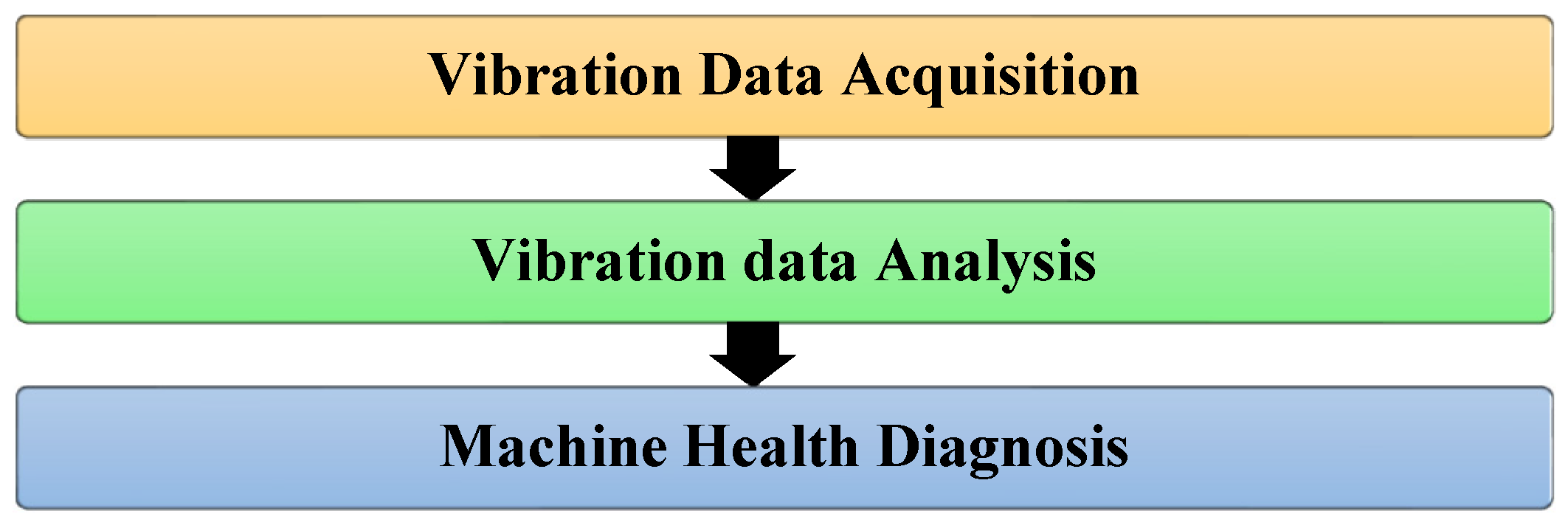
1. Introduction

Rotating machines are essential for a wide range of processes in manufacturing. Thus, their health conditions and availabilities have a direct impact on production plans, excellence, and cost. Maintenance is made by fixing, adjusting, or replacing machine elements, including motors, gearboxes, and bearings to guarantee that a machine remains in a healthy condition. Two types of maintenance are often used, namely corrective and preventive maintenance. Corrective maintenance is usually very expensive as it is accomplished after machine failure. Instead, preventive maintenance is applied to prevent a failure using time-based maintenance (TBM) or condition-based maintenance (CBM). Various studies have shown the economic benefits of applying CBM in several applications of rotating machines [1]. In CBM, maintenance arrangements are made based on the current health condition of a machine, which can be identified through fault diagnosis techniques. Different techniques for machinery fault diagnosis have been developed, including vibration, acoustic emission, electric motor current, and thermography monitoring-based techniques [2,3,4,5,6]. Vibration-based fault diagnosis techniques have been extensively applied and have developed well-acknowledged techniques for machinery maintenance management [7,8,9,10,11].

As presented in Figure 1, the vibration-based fault diagnosis system comprises three stages: (1) data acquisition, to collect input vibration data; (2) data analysis, including preprocessing, filtering, feature extraction, and selection; and (3) machine health diagnosis, to detect and identify faults using a trained classification model.

The acquired vibration data usually comprise a large collection of responses from several sources in the machine accompanied by some background noise. This makes it difficult to use the collected data for machine fault diagnosis directly. Much of the research in this area has focused on computing certain features of the acquired vibration data in the time domain, frequency domain, and time–frequency domain, which can sufficiently describe the signal in essence. Various machine learning methods can be applied to classify a machine’s health condition based on the computed features. It is supposed that if the features are carefully formulated, a machine learning method can train a model that can achieve high classification accuracies of the machine’s health condition. Previous research proposed various techniques that used multiple statistical features extracted in the time domain. These include mean, peak-to-peak value, crest factor, root mean square (RMS), variance, kurtosis, and skewness, as well as other advanced techniques, such as time synchronous averaging (TSA), autoregressive moving average (ARMA), blind source separation (BSS), stochastic parameter, and filtering techniques [1,12,13,14,15,16,17,18,19,20].

Furthermore, various studies have established that frequency domain techniques can reveal information from the time series vibration signal based on frequency characteristics, which are difficult to be observed in the time domain. Fast Fourier transform (FFT) is widely used to transform time domain vibration signals to the frequency domain [21]. Moreover, various features from the vibration frequency spectrum have been applied to represent the health conditions of machines. These include high-frequency resonance, high-order spectra, arithmetic mean, and the RMS of spectral difference techniques [22,23,24,25,26,27]. Moreover, many time–frequency domain techniques have been used for the non-stationary vibration signals that are often produced when machinery faults occur. These include short-time Fourier transform (STFT), wavelet transform (WT), Hilbert–Huang transform (HHT), empirical mode decomposition (EMD), local mean decomposition (LMD), etc. [1,28,29,30,31,32,33,34].

However, extracting and/or selecting the advantageous features which can sufficiently describe the current condition of a machine from such huge and noisy time series vibration datasets is typically a challenging task. The past two decades have seen rapid developments in applying feature-learning techniques that can automatically learn representations of time series datasets to address this problem. A great deal of previous research into the application of feature-learning algorithms for vibration fault diagnosis has focused on deep learning techniques, which learn representations of data by utilising hierarchical multi-layer data processing architectures such as deep neural networks (DNNs) and convolutional neural networks (CNNs) [2,35,36,37]. Furthermore, a renewed interest in converting the 1D vibration signal into a 2D image, which usually offers discriminative characteristics of the vibration signal, has been directed by recent advances in the field of computer vision.

In addition, several attempts have been made to use thermographic analysis and visual inspection for machine fault diagnosis. As described in [38], the thermographic analysis is considered for fault diagnosis given its advantages in being non-invasive and in having a wide range of analyses. It is usually applied using thermographic images taken using a thermographic camera sensor, which is an infrared detector that incorporates both the temperature of the surface and the energy emitted by the targeted object and adapts them into an image called a thermogram. The applications of infrared thermography in machine fault diagnosis and different industrial applications have been reviewed in [39,40].

With the advancements in high-resolution cameras, computer hardware, and software, visual inspection has been used to visually inspect the surface of the components in a machine. This is performed by capturing 2D images from a 3D scene, which are then processed to extract features that can be used to classify the health condition of a machine. In this case, the inspection system defines whether an object or a scene matches a predefined description. Several studies have tested the efficacy of visual inspection in machine fault diagnosis [41,42,43,44,45]. Moreover, the application of optical illumination, image acquisition, image processing, and image analysis in the field of the visual inspection was discussed in [46].

Due to its high performance in fault diagnosis, the image representation of vibration signals is receiving increasing attention from researchers in the field of machinery condition monitoring and diagnosis. In this paper, we review the works associated with vibration image representation-based fault detection and diagnosis for rotating machines to chart the progress in this field. It is hoped that this survey will contribute to a deeper understanding of the techniques used for the image representations of vibration signals and their practice in rotating machine fault diagnosis. The contributions of this paper are as follows:

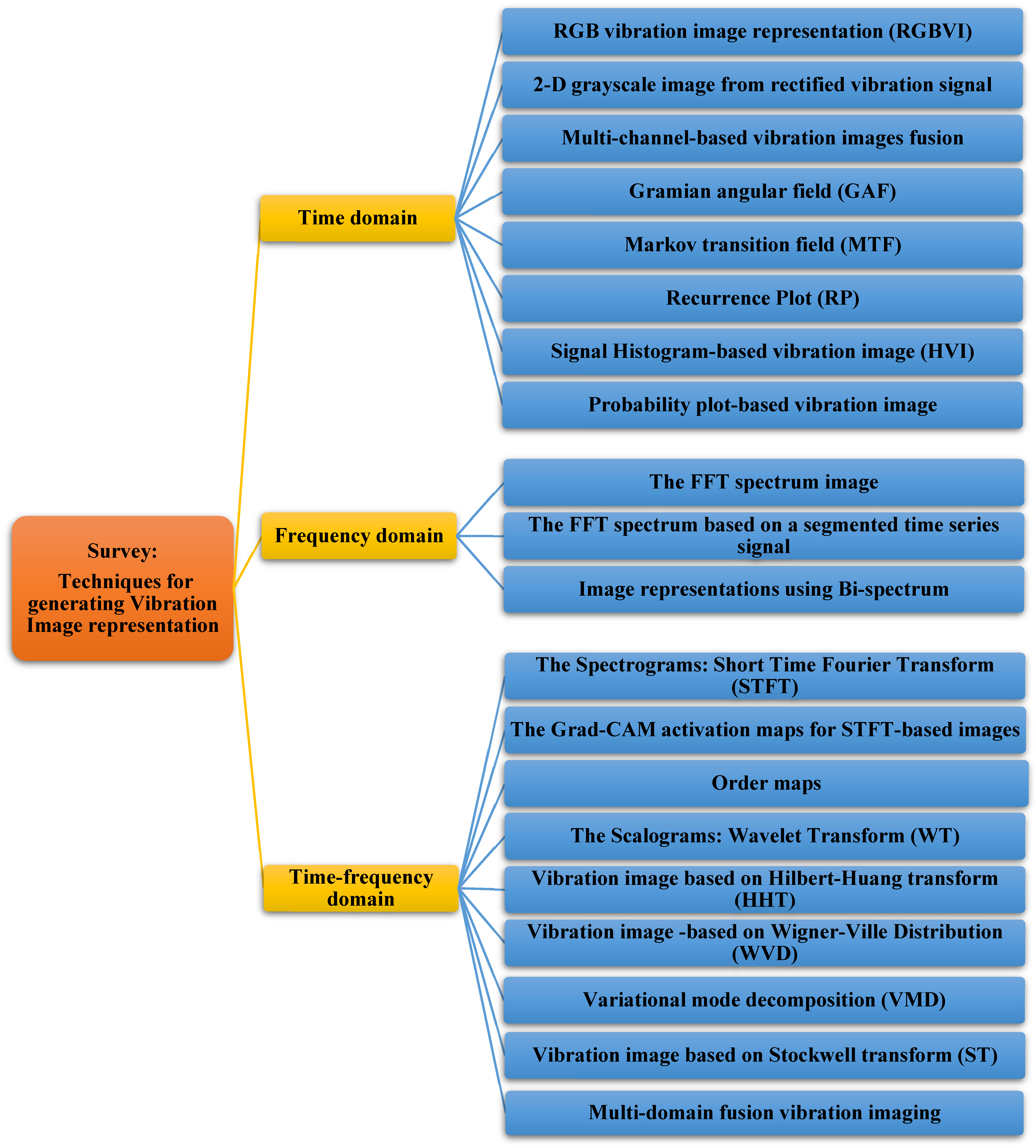
• We summarise the techniques used for the image representations of vibration signals in three signal analysis domains, as shown in Figure 2. The summary includes ten techniques in the time domain, three techniques in the frequency domain, and nine techniques in the time–frequency domain. The latest applications of these techniques in rotating machine fault diagnosis are also discussed.
• With regard to the time domain-based techniques, we present and discuss 2D grayscale, RGBVI, multi-channel fusion, the Gramian transition field, the Markov transition field, the recurrence plot, dominant neighbourhood structure maps (DNS), the signal histogram, and probability plot-based vibration image techniques. With regard to the frequency domain-based techniques, we present and discuss the FFT spectrum and the bi-spectrum, and with regard to the time–frequency domain-based techniques, we present and discuss STFT, STFT-based Grad-CAM, order maps, WT, HHT, Wigner–Ville distribution (WVD), variational mode decomposition (VMD), Stockwell transforms, and multi-domain fusion vibration imaging (MDFVI)-based vibration image representations.

Furthermore, we analyse the literature from four aspects: the targeted rotating machine’s components, the techniques used to produce the vibration image representations, the feature learning, and the classification method, as well as the best classification accuracy achieved. This organisation is expected to be more conducive to the finding of innovations by researchers for improving the accuracy of the rotating machines’ fault detection and diagnosis.

3.

In addition to comprehensively reviewing the development and application of vibration image representation in rotating machine fault diagnosis, we also present the current commonly and publicly available vibration datasets used for fault diagnosis. Finally, we discuss possible future research trends and directions.

The remainder of this paper is organised as follows. Section 2 presents a review of the vibration image representations in the time domain, including descriptions of the techniques and their applications in fault diagnosis. Section 3 is devoted to descriptions of the frequency domain-based techniques for vibration image representations. Section 4 offers descriptions of the time–frequency-based techniques. In Section 5, we discuss the application of vibration image representations in the field of rotating machine fault diagnosis and the performance of these techniques in the field of rotating machine fault diagnosis, and we summarise the limitations of the current techniques and possible future research directions and present the publicly available vibration fault diagnosis datasets.

2. Time Domain-Based Vibration Image Representations

Vibration signals obtained from rotating machines are usually 1D vectors in the time domain as a gathering of time-indexed data points acquired over historical time. Based on the type of transducer employed to acquire the signals, the time-indexed data points represent acceleration, velocity, or proximity. Various techniques have been used to convert the 1D time series vibration signal into a 2D vibration image representation. The following subsections discuss these techniques in more detail.

2.1. Time Series Segmentation-Based Techniques

Time series segmentation is a technique of time domain analysis where the targeted input time series signal is divided into several equal segments. Let $x\left(t\right)\in R^{1xn}$ be the originally collected 1D vibration signal vector, where $n$ represents the length of the vibration signal. To convert $x\left(t\right)\in R^{1xn}$ into a 2D grayscale vibration image representation of $m\times m$ matrix dimensions $I\in R^{mxm}$, first, $x\left(t\right)$ needs to be segmented into m equal segments, where $m=\sqrt{n}$. Then, the sequence of segments is used to construct the 2D grayscale image of the vibration signal using the multiple segments alignment technique such that each segment is aligned as the column or row of the produced vibration image [36]. Figure 3a below shows an example of segmenting $x\left(t\right)$; then, each segment is associated with a column of the produced vibration image $I_c$ such that

$$I_c=\left[\begin{array}{ccc}x{\left(t\right)}_1& \cdots & x{\left(t\right)}_{\left(\left(m-1\right)m\right)+1}\\ ⋮& \ddots & ⋮\\ x{\left(t\right)}_m& \cdots & x_{mm}\end{array}\right]$$

(1)

Figure 3b presents an example of segmenting $x\left(t\right)$; then, each segment is associated with a row of the produced vibration image $I_r$ such that

$$I_r=\left[\begin{array}{ccc}x{\left(t\right)}_1& \cdots & x{\left(t\right)}_m\\ ⋮& \ddots & ⋮\\ x{\left(t\right)}_{\left(\left(m-1\right)m\right)+1}& \cdots & x_{mm}\end{array}\right]$$

(2)

Here, $I_c$ and $I_r$ are the vibration image generated by aligning each segment as a column and as a row, respectively.

The application of these techniques in machine condition monitoring has been considered in several studies. For example, Zhang et al. [47] proposed a method for bearing fault diagnosis using vibration images and a convolutional neural network (CNN). In this technique, the vibration images were produced by dividing the time series signal into $n$ equal segments and aligning each segment as the row of the produced vibration image [47]. Kaplan et al. [48] presented a texture analysis-based method for bearing fault diagnosis. Firstly, in this method, the original vibration signals were converted into grayscale images; then, local binary pattern (LBP) and texture features were computed. With these features, several classifiers were employed to perform the classification task, including random forest (RF), k-nearest neighbour (K-NN), naive Bayes, Bayes net, and artificial intelligence networks (ANNs) [48]. Furthermore, Uddin et al. [49] presented an approach for fault detection and classification of induction motors, utilising 2D texture features and a multiclass support vector machine (MSVM) classifier. In this approach, the raw vibration signals were converted into grayscale vibration images; then, the dominant neighbourhood structure (DNS) was employed to obtain the texture features, which were used as inputs into the MSVM [49]. In [50], the authors proposed a strategy for the fault diagnosis of rolling bearings using grayscale vibration images under an unbalanced dataset. In this strategy, the Wasserstein generative adversarial network with gradient penalty (WGAN-GP) was employed to produce more new data to address the distribution differences as a result of the data imbalance.

Based on the time series segmentation technique, several other developed techniques have been used to enhance the produced 2D grayscale vibration image. The key objective of these techniques is to produce a 2D vibration image with useful discriminative characteristics. The following subsections present the details of these techniques.

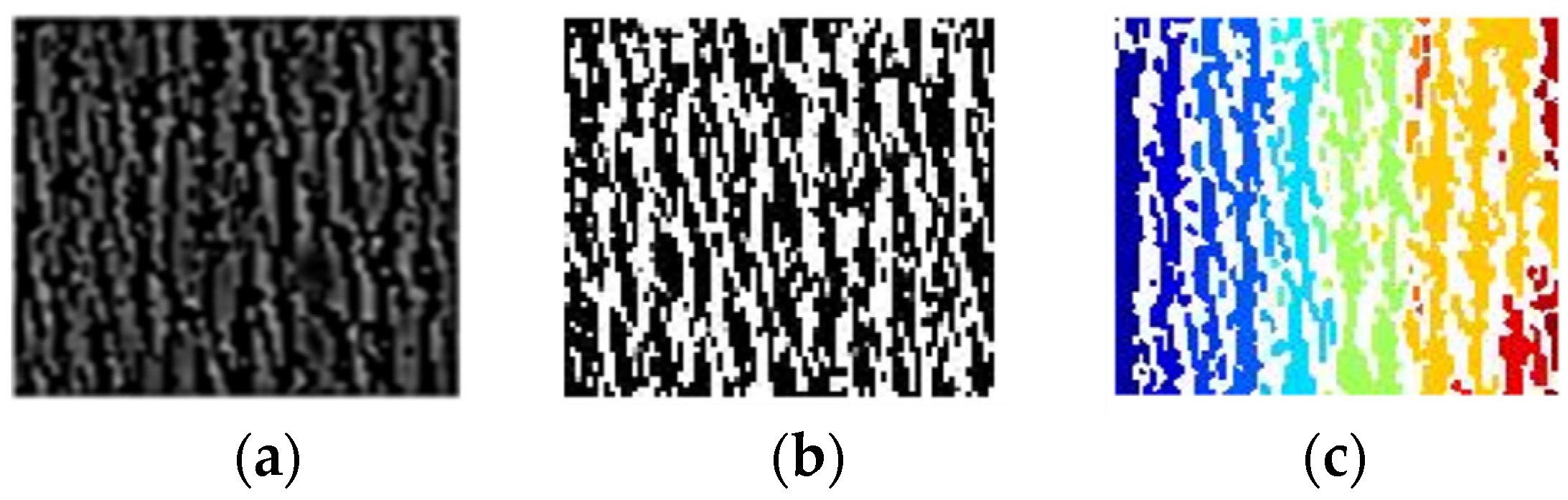
2.1.1. RGB Vibration Image Representation (RGBVI)

In this technique, the generated grayscale image is further processed using the following three steps [36]:

• Convert the grayscale image into a binary image by converting all pixels in the grayscale image with values greater than 1 into white and all other pixels into black.
• Generate a label matrix from the connected components in the binary image with unique values.
• Convert the created label matrix into an RGB-based colour image with a set of colour and texture features of the labeled regions.

Moving on now to consider the application of the RBGVI in machine fault diagnosis, Ahmed et al. [36] employed the produced RGBVIs of bearing vibration signals as inputs into a CNN architecture to train, validate, and classify bearing health conditions [36]. Figure 4 below shows examples of the generated vibration images from bearing vibration with the normal condition, including the grayscale image that was generated using the time series segmentation technique described in Section 2.1 above, the binary image, and the RGB-based colour image.

Figure 5 depicts examples of the generated vibration images using the RGB-based connected components vibration image technique from bearing vibration with six health conditions: two normal conditions, including the brand new bearing (NO) and the bearing in service for some time but in a good condition (NW), and four fault conditions with inner race fault (IR), outer race fault (OR), rolling element fault (RE), and cage fault (CA) [36].

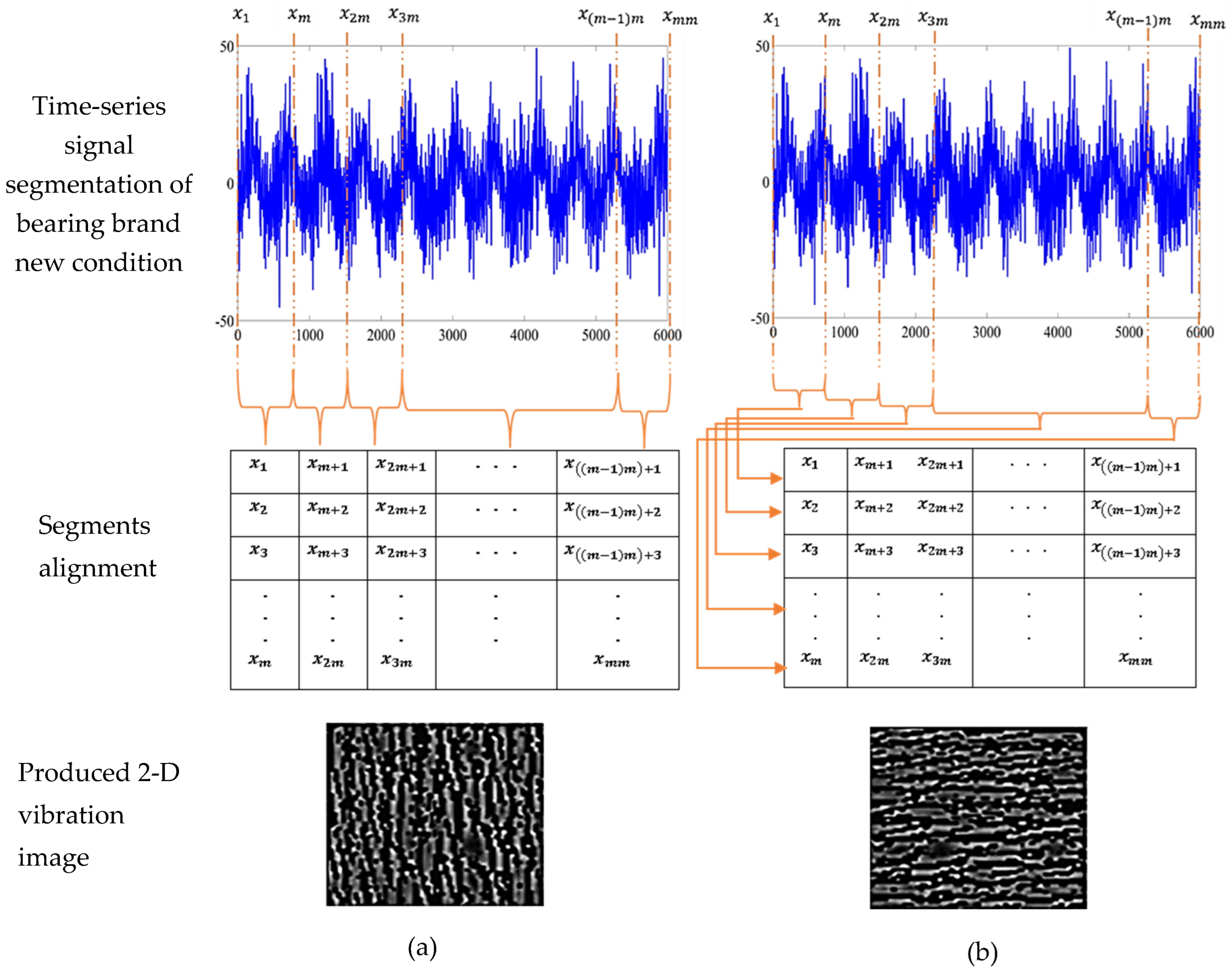
2.1.2. Constructing a 2D Grayscale Image from a Rectified Vibration Signal

Firstly, in this technique, the vibration signal $x\left(t\right)$ is rectified to invert the negative values to positive values [51]. Then, the rectified signal is divided into equal-length segments where the length of each segment $l_s$ is equal to the number of samples in one revolution of the vibration waveform such that

$$l_s=round\left(\frac{60f_s}{S{h}_s}, number of pixels\right)$$

(3)

Here, $f_s$ represents the sampling frequency and $S{h}_s$ is the shaft speed. The value of $l_s$ is rounded to the nearest multiple numbers of pixels as required by the designed system. For example, in [51] the value of $l_s$ is rounded to 3 as the authors used a local binary pattern (LBP) operator that works with 3 × 3 pixels blocks. The LBP of a pixel in an image is calculated by comparing it with its neighbours such that

$$LB{P}_{P,R}={{\displaystyle \sum }}_{p=0}^{P-1}s\left(g_p-g_c\right)2^p, s\left(x\right)=\left\{\begin{array}{c}1, x\ge 0\\ 0, x<0\end{array}\right.$$

(4)

Here, $P$ is the total number of neighbours, $R$ is the radius of the neighbourhood, $g_c$ represents the gray value of the central pixel, and $g_p$ is the value of its neighbours [52]. This technique is validated on bearing fault datasets with different shaft speeds. Figure 6 below presents examples of the generated vibration image using this technique from bearing vibration acceleration signals for 1748 rpm with inner race fault, outer race fault, and ball fault conditions. With these generated vibration images, a k-NN was employed to perform the classification task.

2.2. Multi-Channel-Based Vibration Images Fusion

This method was developed based on three channels that were used to collect vibration samples [53]. To generate a 3M × N-sized fused vibration image from the three vibration signals collected using the three channels, the following steps are performed.

• The three raw signals are randomly segmented to obtain several scalars $s\left(k, i\right)$. Here, $k=1, 2, 3$ is the signal collection channel, and $i=1, 2, 3, \dots , M\times N$;
• The scalar products $S\left(k, i\right)$ can be computed using the following equation

  $$S\left(k, i\right)=s\left(k, i\right). s\left(k, i\right)$$

  (5)
• The pixel value of the feature images $F\left(m, n\right)$ can be calculated using the following equation

  $$F\left(m, n\right)=unit8(255\times \frac{S\{k, \left(m-k\right)\times \frac{N}{3+1})\}}{Max S\left\{k\right\}})$$

  (6)

Here, $m=1, 2, \dots , 3M$ and $n=1,2, \dots , N$.

This method was verified on vibration datasets collected from a wind power test rig with several complex faults of the bearings and gears and a centrifugal pump test rig with cavitation, impeller unbalance, and shaft misalignment. In [53], the produced vibration images were used as inputs into a bottleneck layer optimized CNN (MB-CNN) to further perform feature learning from the produced vibration images and to classify the type of fault corresponding to each signal.

Figure 7 shows an example of the composite image with an inner bearing fault produced from three feature maps using the data described in Section 2.1.1.

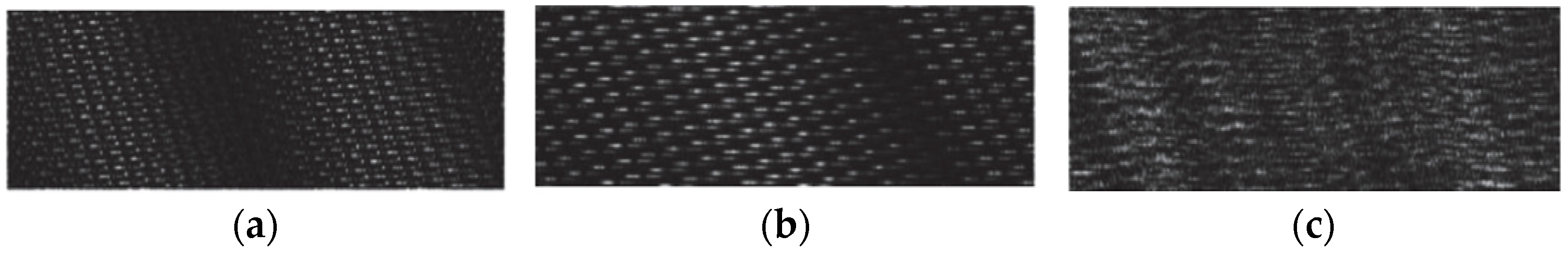
2.3. Gramian Angular Field (GAF)

To encode the vibration time series to a vibration image using GAF, the following steps are performed [54,55]:

• Given the original collected 1D time series vibration $x\left(t\right)\in R^{1xn}$ where $n$ represents the length of the vibration signal, first $x\left(t\right)$ is rescaled so all values are in the range [−1, 1] such that

  $$\tilde{x}=\frac{\left(x_i-\max \left(x\right)+x_i-\min \left(x\right)\right)}{\max \left(x\right)-\min \left(x\right)}$$

  (7)
• The rescaled time series $\tilde{x}$ is represented in polar coordinates by encoding the value as the angular cosine and the time stamp as the radius such that

  $$\left\{\begin{array}{c}\varnothing =\arccos \left({\tilde{x}}_i\right),-1\le {\tilde{x}}_i\le 1, {\tilde{x}}_i\in \tilde{x} \\ r=\frac{t_i}{N}, t_i\in \mathrm{\mathbb{N}} \end{array}\right.$$

  (8)

Here, $t_i$ is the time stamp, and $N$ represents a constant factor to regularise the span of the polar coordinate system.

3.

The angular perspective is exploited in view of the trigonometric sum between each point to find the time-based correlation inside different time intervals. Thus, the GAF matrix can be defined using the following equation

$$GAF=\left[\begin{array}{ccc}\cos \left({\varnothing }_1+{\varnothing }_1\right)& \cdots & \cos \left({\varnothing }_1+{\varnothing }_n\right)\\ ⋮& \ddots & ⋮\\ \cos \left({\varnothing }_n+{\varnothing }_1\right)& \cdots & \cos \left({\varnothing }_n+{\varnothing }_n\right)\end{array}\right]$$

(9)

$$={\tilde{x}}^{\prime }. \tilde{x}-{\sqrt{1-{\tilde{x}}^2}}^{\prime }.\sqrt{1-{\tilde{x}}^2}$$

(10)

Figure 8 shows examples of the generated vibration images using the GAF from the bearing vibration with the six health conditions described in Section 2.1.1 above.

To date, several studies have investigated the application of the GAF technique in machine fault diagnosis. For instance, Garcia et al. [55] investigated several encoding algorithms, including GAF, to produce images from highly complex vibration measurements of real helicopter flight tests; then, they used these images as inputs into a deep learning architecture, namely the convolutional auto-encoder (CAE) and CNN [55]. Moreover, Han et al. [56] conducted several experiments to test the efficacy of GAF-based vibration images as inputs into capsule networks in bearing fault diagnosis [56].

2.4. Markov Transition Field (MTF)

The MTF technique produces images that contain the transition probabilities of the inputted time series vibration signal $x\left(t\right)$ by performing the following steps [54,55,56,57]:

• Construct a $Q\times Q$ Markov transition matrix $W$ by recognising the Q quantile bins of the input signal $x\left(t\right)$ and allocate each element $x_i$ in $x\left(t\right)$ to its corresponding quantile $q_i$ such that

  $$W=\left[\begin{array}{ccc}{w}_{11}& \cdots & w_{1Q}\\ ⋮& \ddots & ⋮\\ w_{Q1}& \cdots & w_{QQ}\end{array}\right]$$

  (11)

Here, $w_{ij}$ is the probability of the element $q_i$ being transferred to $q_j$ and ${\displaystyle \sum }_{j=1}^Q{w}_{ij}=1$.

2.

The MTF $N X N$-sized matrix is computed using the following equation

$$MTF=\left[\begin{array}{ccc}{w}_{ij}|x_1\in q_i,x_1\in q_j & \cdots & w_{ij}|x_1\in q_i,x_n\in q_j\\ ⋮& \ddots & ⋮\\ w_{ij}|x_n\in q_i,x_1\in q_j& \cdots & w_{ij}|x_n\in q_i,x_n\in q_j\end{array}\right]$$

(12)

Figure 9 shows examples of the generated vibration images using the MTF from the bearing vibration with the six health conditions described in Section 2.1.1 above.

The application of MTF in machine fault diagnosis has been considered in quite a few studies [55,56,57]. In [55], the MTF-based vibration images were used as inputs into the CAE and CNN to test the classification accuracy of vibration images with normal and anomalous conditions. In [56], three scenarios of vibration images were produced using GAF, MTF, and GAF + MTF as inputs into the capsule network for bearing fault diagnosis. In [57], MTF-based vibration images were used as inputs into a ResNet-based CNN architecture to train a model for bearing fault diagnosis.

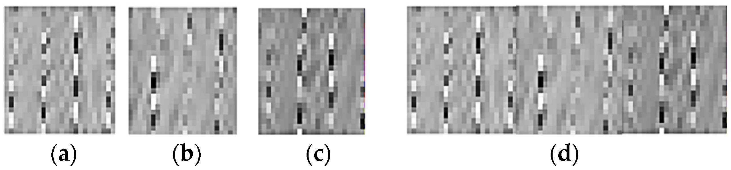
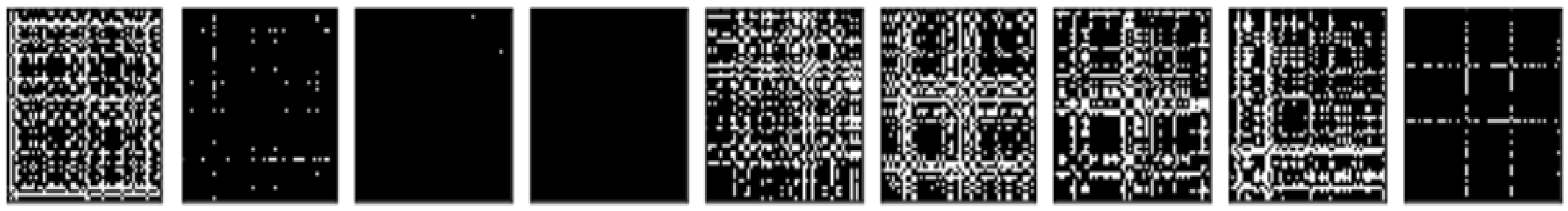
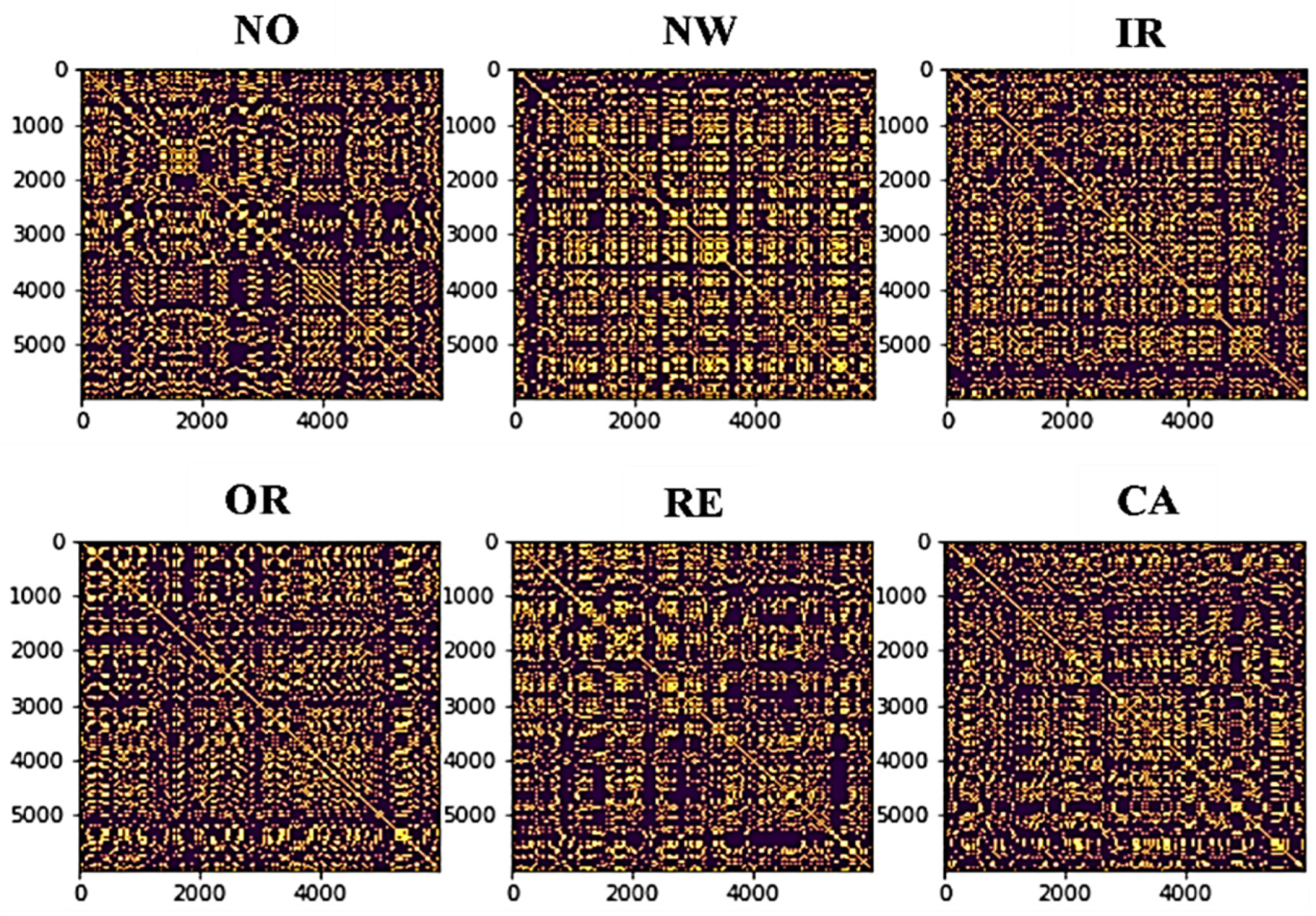
2.5. Recurrence Plot (RP)

The recurrence plot (RP) is a technique that transforms a time series into an image of recurrences, which visualise the recurrent behaviors in the time domain [55,58,59,60]. This image is able to divulge in which elements some routes return to a previously visited state. The mathematical expression of RP is shown in the following equation,

$$R{P}_{ij}=\theta \left(ϵ-\Vert {\overrightarrow{x}}_i-{\overrightarrow{x}}_j\Vert \right), \overrightarrow{x}\in {\mathcal{R}}^m, i,j=1\dots N$$

(13)

Here, ${\overrightarrow{x}}_i$ and ${\overrightarrow{x}}_j$ are the subsequentness detected at the positions $i$ and $j$, respectively; $\theta$ is the Heaviside function, $ϵ$ is a threshold, and N is the number of states. The recurrence plot represents a binary image in which dots only specify whether there is a reappearance of a state or not. Figure 10 presents the plots for nine-time series of bearing vibration signals with different health conditions from the bearing vibration data described in Section 2.1.1.

Figure 11 shows examples of the generated vibration image using the RP technique with a distance threshold for the bearing vibration with six health conditions. Moreover, Figure 12 depicts examples of the generated vibration image using the RP technique with a point threshold for the same bearing vibration.

A search of the literature revealed a few studies that considered the application of RP in machine fault diagnosis. For example, in [55] several encoding algorithms, including RP, were tested to produce images from the vibration signals of real helicopter flight tests; then, these images were used as inputs into a CAE-based deep architecture for fault diagnosis. In [60], the RP and quantification techniques were utilised for bearing fault diagnosis using vibration signals. It was shown that several of the recurrence indicators, such as determinism, laminarity, entropy, average diagonal line, and trapping time could be used for bearing fault diagnosis [60].

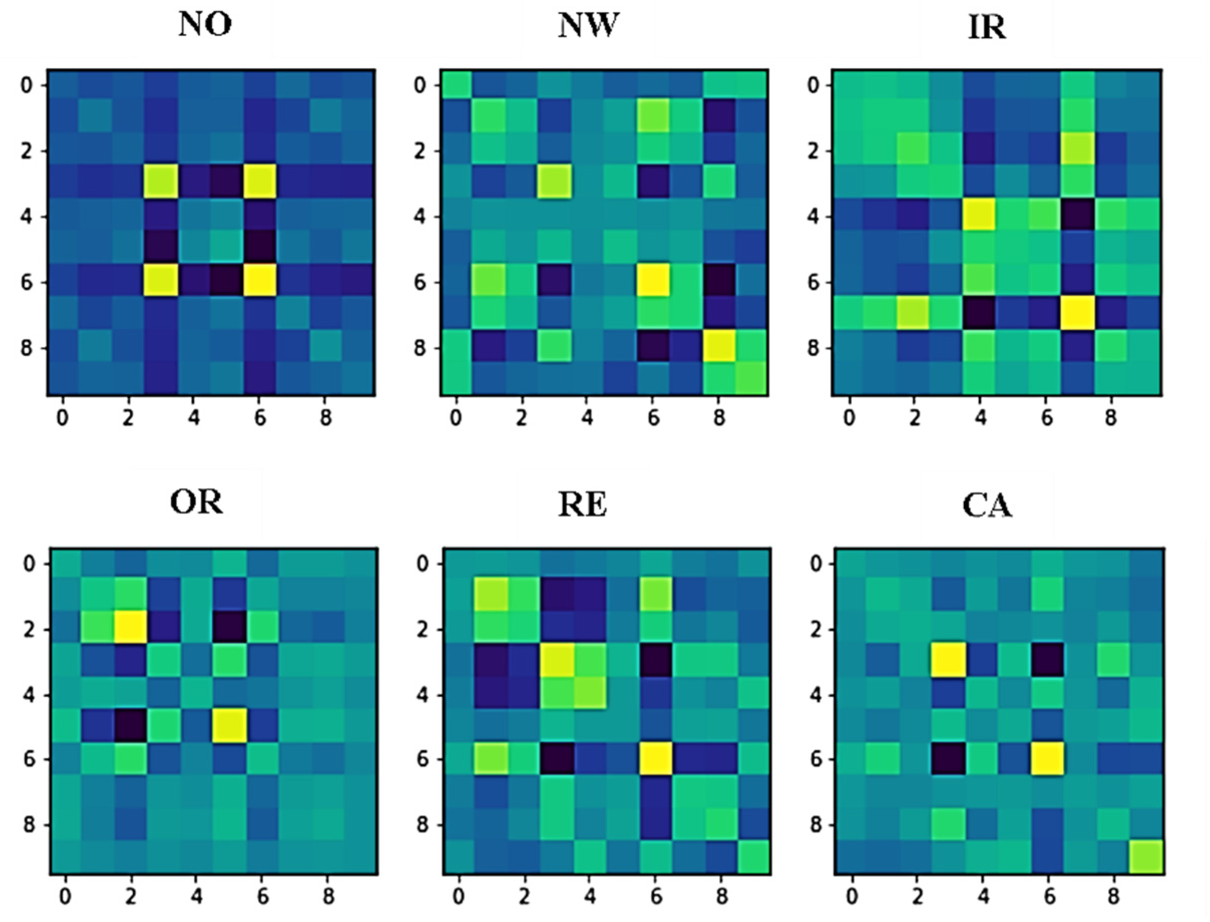
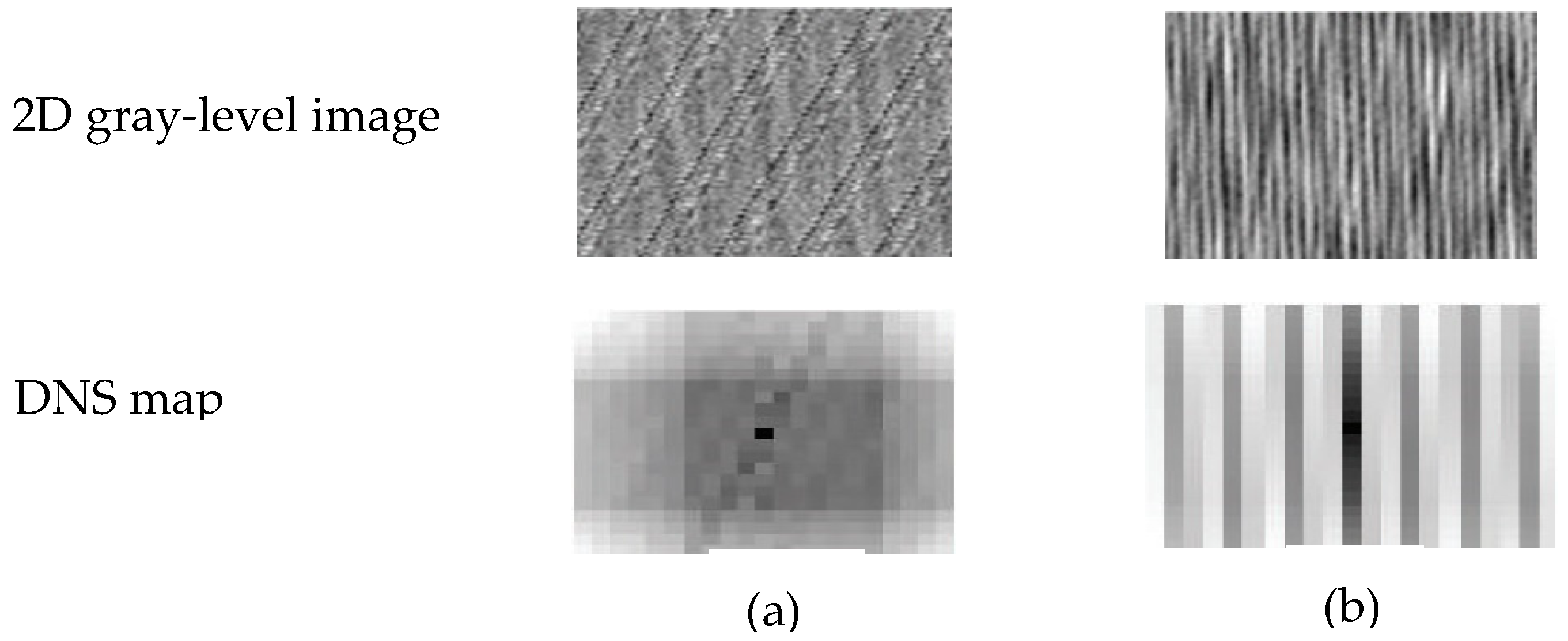
2.6. DNS Map-Based 2D Vibration Image

This technique generates 2D texture features from the time series vibration signal using the following steps [49].

• Convert the 1D time series vibration signal to a 2D gray-level image. Firstly, in this step, the amplitude of each sample of the time series vibration signal is normalised; then, each sample is assigned the intensity of the corresponding pixel.
• Produce a dominant neighbourhood structure (DNS) map to extract texture features from the 2D gray-level image.

Figure 13 shows examples of the generated 2D gray-level images and their corresponding 2D DNS map [49].

This technique is used for the fault classification of induction motors [49]. The DNS map-based extracted texture features were reduced using PCA, and then, multi-class support vector machines (MCSVMs) were employed to identify induction motor faults.

2.7. Signal Histogram-Based Vibration Image (HVI)

The histogram-based vibration image is developed to describe the two channels of vibration signal and the joint relationship between them concurrently [61]. The HVI can be obtained as follows.

• Compute the vibration image center $\left(\overline{x}, \overline{y}\right)$ for the $\left(x_i, y_i\right)$ vibration sample points, where $i=1, 2, \dots , N,$ and $N$ is the total number of vibration sample points such that

  $$\overline{x}=\frac{1}{N}{{\displaystyle \sum }}_i{x}_i$$

  (14)

  $$\overline{y}=\frac{1}{N}{{\displaystyle \sum }}_i{y}_i$$

  (15)
• Eliminate the unexpected outliers by drawing a vibration circle with the center of $\left(\overline{x}, \overline{y}\right)$ and $R$ as the radius, which can be computed as follows

  $$R=A_m subject to:T=\frac{count\left(A_i\le A_m\right)}{N}$$

  (16)

Here, $T$ is the ratio of the sample points to be retained and is set to 95%, and $A_i$ is the Euclidian distance between the center and all the vibration sample points.

3.

Construct the histogram feature by dividing the vibration circle into $\mathrm{N}$ rings. Here, the $k-th$ bin value of the histogram is set to the number of sample points within the $k-th$ ring.

4.

Normalise the histogram such that

$$zero\left(x\right)=\left\{\begin{array}{c}1, x=0\\ 0, x\ne 0\end{array}\right.$$

(17)

$$hvi\left(k\right)={{\displaystyle \sum }}_{i}zero\left(z_i-k\right)$$

(18)

Here, $z_i$ is the ith sample point located in the z_ith ring. Figure 14 shows a diagram that represents the HVI technique.

Moreover, the oriented histogram-based vibration image (HOVI) that represents the distribution of the vibration sample points in various directions is developed in [61]. The HOVI is based on dividing the phase space ${\theta }_i$ into $p$ intervals, where ${\theta }_i$ can be calculated using the following equation.

$${\theta }_i=\arg \left(x_i-\overline{x}\right)+\left(y_i-\overline{y}\right), {\theta }_i\in \left[0, 2\pi \right]$$

(19)

In HOVI, the bin value of the histogram is computed as follows.

$$hovi\left(k\right)=\frac{{{\displaystyle \sum }}_i{A}_i zero\left(z_i-k\right)}{{{\displaystyle \sum }}_i zero\left(z_i-k\right)}$$

(20)

Here, $z_i$ can be computed using the following equation

$$z_i=\left[\frac{{\theta }_i}{\frac{2\pi }{p}}\right]$$

(21)

So far, very little attention has been paid to the application of HVI and HOVI in machine fault diagnosis. For instance, to validate the efficacy of HVI and HOVI in machine fault diagnosis, the authors in [61] conducted several experiments on a dataset with four types of faults collected from a test rig of a magnetic bearing-rotor system. With the produced vibration images, a two-layer AdaBoost was employed to perform the fault diagnosis task. Medina et al. [62] proposed two methods for gearbox vibration signal-based fault diagnosis using a symbolic dynamics algorithm. The first method, which is called SDA, extracts the symbols’ histogram directly from a Poincaré plot produced from a time series vibration signal. The second method, PSDA, extracts the phase-space subdivision-based symbols’ histogram from a Poincaré plot generated from a peaks sequence obtained from a time series vibration signal. A vibration signal dataset with 10 classes of faults acquired from a gearbox was used to validate these methods and the classification task was performed using an MSVM classifier [62].

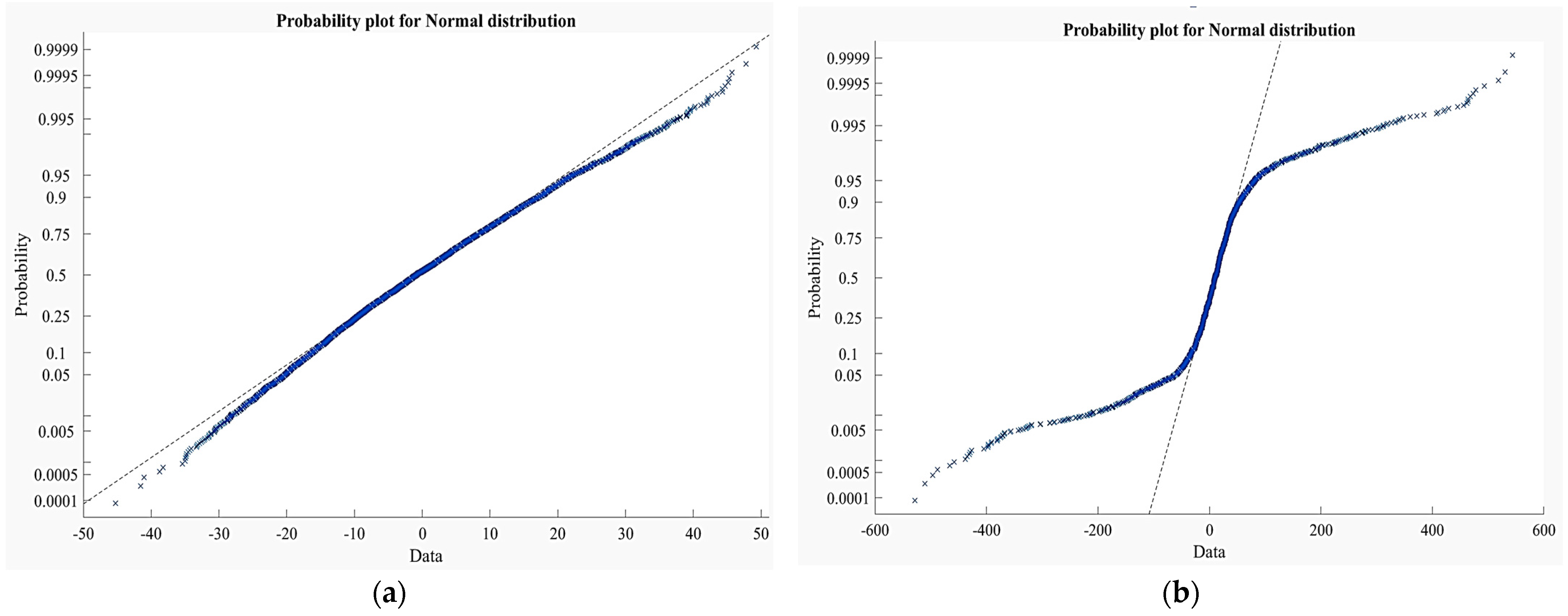
2.8. Probability Plot-Based Vibration Image

In this technique, the probability plot of the time series vibration data is performed according to a theoretical data distribution, such as Normal and Weibull. The resulting points of the plot would be bordered and arranged in a straight line where any nonconformity from this bordered straight line designates a deviation from the distribution. By using this merit, the different vibration signals with faults can be diagnosed, where the further the probability plot results differ from the straight line the better the detection and the diagnosis of the faults that can be achieved [63].

The highest correlation coefficient is chosen to produce the best features of the vibration image through the probability plot. The vertical axis of the produced vibration image includes ordered response values, while the horizontal axis comprises ordered statistic medians $Me{d}_i$ for the given distribution, which can be computed as follows.

$$Me{d}_i=f\left(M{u}_i\right)$$

(22)

Here, $f$ is the percent point function for the distribution, and $M{u}_i$ is the uniform order statistics median, which can be defined using the following equation [49].

$$\left\{\begin{array}{l}M{u}_i=1-M{u}_i ;\hspace{1em}for i=1\\ M{u}_i=\frac{\left(i-0.3175\right)}{\left(n+0.365\right)} ;\hspace{1em}for i=2,3, \dots , n-1\\ M{u}_i={0.5}^{\left(\frac{1}{n}\right)} ;\hspace{1em}for i=n\end{array}\right.$$

(23)

Figure 15 shows examples of the probability plot based-images for bearing vibration signals with the normal condition and inner race fault from the data described in Section 2.1.1.

The application of the probability plot in machine fault diagnosis has been considered in several studies [63,64,65,66,67,68]. In [63], the probability plots constructed from bearing vibration signals collected under constant and variable speed conditions were used as input images in the absolute value PCA for bearing fault diagnosis.

3. Frequency Domain-Based Vibration Image Representations

The time series vibration signals are usually produced by several elements of the rotating machine, such as the bearings, gears, and shaft. In a single motion, each element generates a sine wave with a single frequency and amplitude, whereas other elements add more frequencies and amplitudes. These frequencies are not easily seen in the time domain. The frequency spectrum of the time series signals makes it easy to see this range of frequencies. Fourier analysis is often used to transform the time domain vibration signals to the frequency domain [1]. Moreover, several techniques within the frequency domain were developed to convert the 1D time series vibration signal into a 2D vibration image representation. The following subsections briefly describe these techniques.

3.1. The FFT Spectrum Image

In this technique, the fast Fourier transform spectrums of the vibration signals are used as images [69]. The FFT algorithm calculates the n-point complex discrete Fourier transform (DFT) of the time series signal $x\left(t\right)$. The sampled points of $x\left(t\right)$ are divided into two parts: $x_{even}$ ($x_0, x_2, x_4, \dots )$, which contains the collected even-numbered sampled points, and $x_{odd}$ ($x_1, x_3, x_5, \dots )$, which contains the odd-numbered sampled points, each of which has half of the total sampled points such that

$$x{\left(t\right)}_{DFT}\left(k\right)=DF{T}_{\frac{N}{2}}\left\{x_{even}\left(m\right), k\right\}+W_N^k.DF{T}_{\frac{N}{2}}\left\{x_{odd}\left(m\right),k\right\}, k=0, 1, \dots , N-1$$

(24)

To obtain the FFT spectrum image, the magnitude of the DFT, i.e., the absolute value of the DFT is used. Figure 16 shows examples of time series vibration signals and their corresponding FFT spectrum images for the inner race, outer race, and rolling element fault. Those readers who are interested in more details on the mathematical formulation of FFT may be referred to [1,70,71]. Moreover, the application of FFT-based vibration spectrum images in machine fault diagnosis was studied extensively in [69,71,72,73,74,75,76,77].

3.2. The FFT Spectrum Image Based on Segmented Time Series Signal

Firstly, in this technique, the time series signal is divided into time segments using a window of size $W$ samples [74]. Then, the time segments are stacked in an image $I_{x\left(t\right)}$ such that

$$I_{x\left(t\right)}=\left\{x_u\left(w\right)\right\}$$

(25)

Here, $w=1, 2, \dots , W$ and $u=1, 2, \dots , U$ where $U$ is the number of time segments.

Afterwards, the FFT is used to form a spectrum image $I_f$ from $I_{x\left(t\right)}$. Finally, the obtained spectrum image $I_f$ is enhanced using a 2D averaging filter and a binary threshold.

3.3. Image Representations Using Bi-Spectrum

In this technique, the bi-spectrum, also called the third-order spectrum, which is the Fourier transform of the third-order statistics, is employed to transform the 1D time series vibration signal into a 2D vibration image [78,79]. It often offers additional diagnostic information to that offered by the power spectrum of the signals containing non-Gaussian components [1]. The bi-spectrum can be normalised with respect to the power spectrum to produce bi-coherence, which is useful in detecting quadratic phase coupling. The bi-spectrum ($B_s$) can be expressed mathematically using the following equation.

$$B_s\left(f_1,f_2\right)=E(X\left(f_1\right) X\left(f_2\right)X^{\ast }\left(f_1+f_2\right)$$

(26)

Figure 17 shows examples of the produced vibration images using bi-spectrum counter maps of time series vibration signals with different conditions, including bearing roller wearing fault, inner race wearing fault, outer race wearing fault, normal condition, and centrifugal pump impeller wearing fault condition [80].

Many studies have begun to examine the application of frequency domain-based vibration images in machine fault diagnosis. For example, Li et al. [69] presented a method for bearing fault diagnosis using spectrum images of vibration signals obtained by performing the FFT technique. Then, the obtained vibration images were processed using 2DPCA to reduce the dimensions. Finally, a minimum distance technique was employed to perform the classification task [69]. Liang et al. [72] proposed a method for bearing fault diagnosis using the CNN. In this technique, the time series vibration signals were converted into 2D frequency spectrums using FFT and then used as inputs into the CNN to train a classification model for bearing fault diagnosis [72]. In [73], a vibration spectrum imaging-based technique for bearing fault classification was proposed. Firstly, in this technique, the original vibration signals were time-segmented. Then, the spectral contents of each time segment were computed and normalised to form a spectral image using FFT. Then, an image enhancement process was performed to enhance the obtained spectral images. Finally, an ANN was employed to train a model for bearing fault classification. In the same vein, Youcef et al. presented a method that used spectral images as inputs into a CNN classifier to train a model for bearing fault classification [74].

Furthermore, Huang et al. proposed a technique for fan fault diagnosis using vibration spectral image, PCA, and an ANN [75]. Similarly, Qiu et al. presented a method for bearing fault diagnosis using adjusted vibration spectrums, 2DPCA, and NNC [76]. In [80], the authors proposed a technique for rotating machine fault diagnosis using bi-spectrum-based vibration images; feature extraction, using speeded-up robust features (SURF); dimensionality reduction based on t-distributed stochastic neighbour embedding (t-SNE); and fault identification based on the probabilistic neural network (PNN).

4. Time–Frequency Domain-Based Vibration Image Representations

The time-frequency domain analysis has been utilised for non-stationary vibration waveforms, which are very common when machinery faults happen. Several techniques within the time-frequency domain were used to produce 2D vibration image representations from the 1D time series vibration signals. The following subsections briefly describe these techniques.

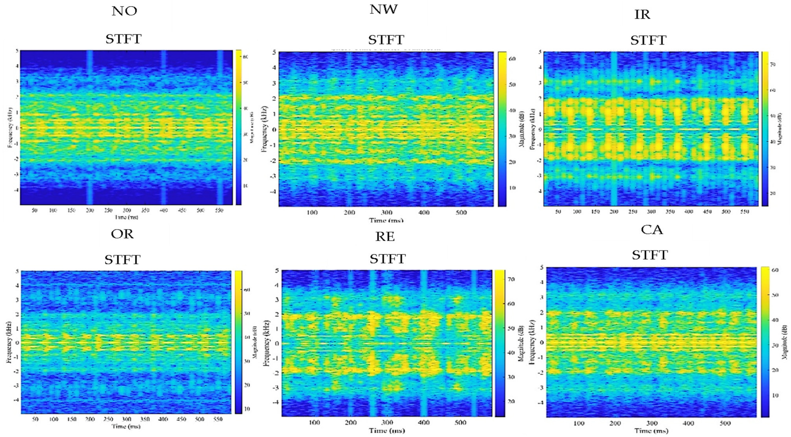
4.1. Short-Time Fourier Transform (STFT)

The short-time Fourier transform (STFT) is a form of the Fourier transform which lets one examine a non-stationary vibration signal in the time-frequency domain [81]. The STFT of a time series vibration signal $x\left(t\right)$ can be computed using the following equation.

$$STF{T}_{x\left(t\right)}\left(t,w\right)={{\displaystyle \int }}_{-\infty }^{+\infty }x\left(t\right)w\left(t-\tau \right)exp\left(-jwt\right)d\tau$$

(27)

Here, $w\left(\tau \right)$ is a window function and $\tau$ is a time variable. In STFT, the signal is decomposed into shorter equal segments via a time-localised window function such as the Gaussian and Hamming window, and it then accomplishes the DFT on each segment individually. The time-frequency spectrum is the collection of the DFTs of the whole segments. The spectrogram or sonogram is often used to estimate the frequency content of the STFT-based signal. It is a graphical image of the signal that estimates the energy distribution of the signal within the time-frequency domain. The spectrogram can be mathematically represented by the magnitude squared of STFT such that

$$Spec{t}_{x\left(n\right)}\left(n,w\right)=\left| STF{T}_{x\left(n\right)}{\left(n,w\right)}^2\right|$$

(28)

Figure 18 presents examples of the generated vibration images using STFT from the bearing vibration signals with six health conditions, as described in Section 2.1.1 above.

Numerous studies employed the STFT-based images as inputs into a classifier to perform the fault diagnosis task [82,83,84,85,86,87,88], while other studies have attempted to produce features based on the STFT images of the original vibration signals for fault diagnosis. The following subsections highlight two of these techniques.

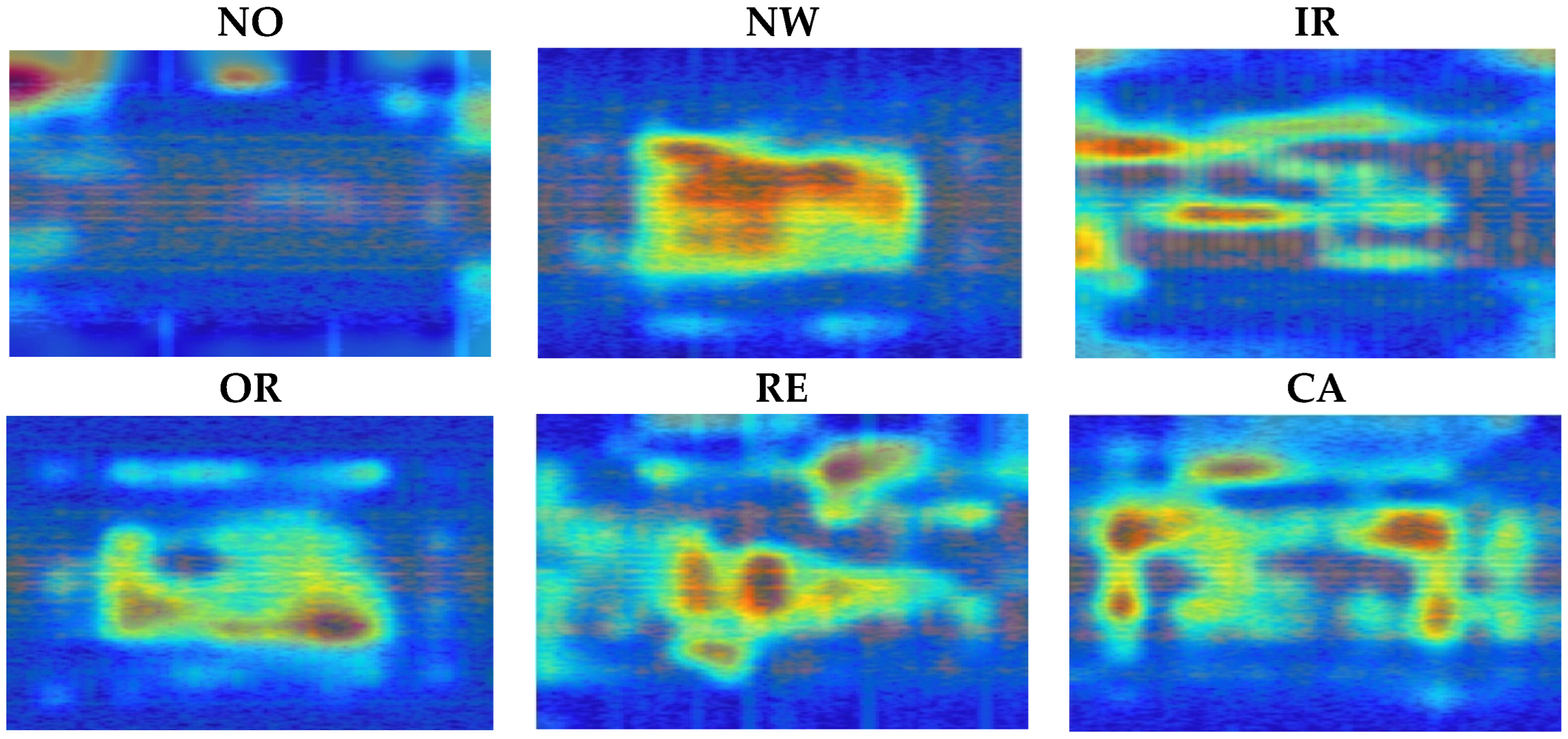
4.1.1. The Grad-CAM Activation Maps for STFT-Based Images

The use of the gradient-weight class activation mapping (Grad-CAM) algorithm, along with the STFT-based 2D images, was proposed by Liefstingh et al. in [89] to recognise elements of the input spectrogram that contribute to each class attribution of the input signals of bearings. The Grad-CAM utilises the gradient information flowing in the last convolutional layer of the CNN [90]. By using a trained neural network, the Grad-CAM highlights which areas of an input image are of importance for classification [91]. For example, Figure 19 presents examples of the generated Grad-CAM activation maps using a pre-trained network, namely squeezenet [92], for the STFT-based vibration images produced from the bearing vibration signals with six health conditions in Figure 18.

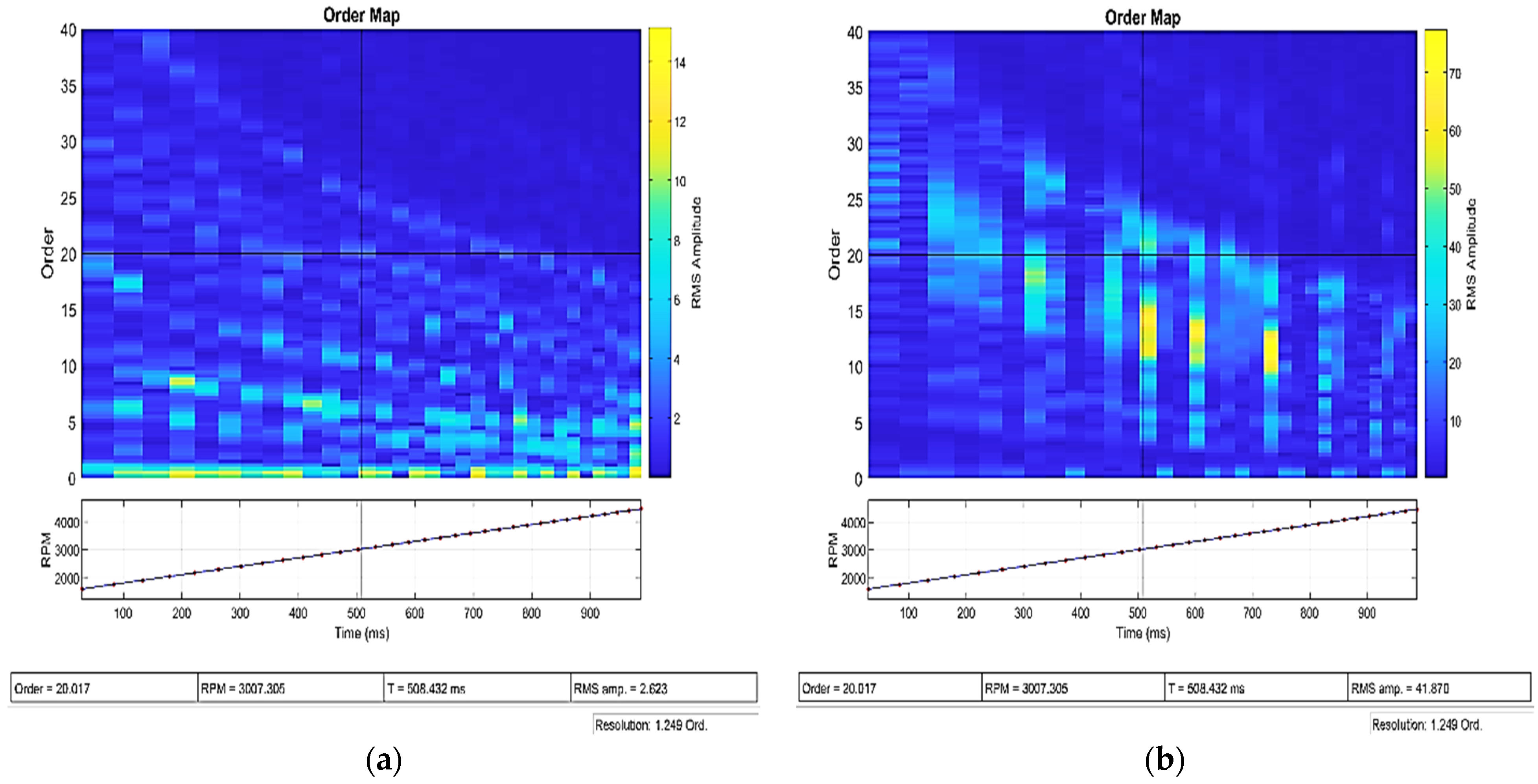
4.1.2. Order Maps

As described by Tayyab et al. [93], order maps can be computed using the following three steps:

• Tachometer signal processing and rpm extraction.
• Synchronous resampling in the order domain.
• STFT of resampled signal in the order domain.

Figure 20 shows examples of the order maps of two bearing vibration signals with normal and inner race fault conditions under variable speeds (25–75 rpm). In [93], this technique is used for rolling element bearing diagnosis under variable speeds and loads. The order maps show the different patterns for different types of faults. Therefore, they are used as inputs into a CNN for fault diagnosis.

4.2. Wavelet Transform (WT)

The WT is an alternative technique to the STFT for the analysis of non-stationary signals. It is adaptable to a wide range of frequencies and time-based resolutions. Unlike the window used by STFT, the WT utilises wavelet families with fixed shapes, such as Haar, Symlets, and Daubechies. The main wavelet function $\psi \left(t\right)$ can be computed as follows.

$${\psi }_{s,\tau }\left(t\right)=\frac{1}{\sqrt{s}} \psi \left(\frac{t-\tau }{s}\right),$$

(29)

Here, $s$ is the scaling parameter, $t$ is the time, and $\tau$ represents the transformation parameter. In the original wavelet, $s=1$ and $\tau =0$. There are three key transforms in wavelets, namely continuous wavelet transform (CWT), discrete wavelet transform (DWT), and wavelet packet transform (WPT) [94,95,96,97,98,99]. Of these, the CWT was used by many researchers to generate vibration image representations.

The CWT can be computed using the following equation

$$W_{(x\left(t\right)}\left(s, \tau \right)=\frac{1}{\sqrt{s}} \int x\left(t\right){\psi }^{\ast }(\frac{t-\tau }{s})dt$$

(30)

Here, ${\psi }^{\ast }$ represents the complex conjugate of $\psi \left(t\right)$, which can be shifted using the translation parameter $\tau$ and scaled using the scale parameter $s$. The computed coefficients define the correlation between the waveform and the wavelet utilised at the performed translations and scales. These coefficients are usually presented in a scalogram, which characterises the percentage of the energy for each coefficient. Figure 21 shows examples of the produced scalograms using CWT with complex-valued Gaussian wavelets from the bearing vibration signals with six health conditions that were described in Section 2.1.1 above. The wavelet coefficients find the differences in the vibration waveform of the six vibration signal conditions.

The application of the WT and the scalograms in machine condition monitoring has been considered in various studies. For example, Shi et al. [100] presented a technique for bearing fault diagnosis using CWT and a residual dilated pyramid network, and a full convolutional denoising autoencoder (RDPN-FCDAE). Firstly, in this technique, the CWT is employed to convert the time series vibration signals into vibration images. Then, the produced vibration images were used as inputs into the RDPN-FCDAE for feature learning and fault classification. In [101], a method for bearing fault diagnosis using CWT, DCNN, and random forest (RF) ensemble learning is proposed. In this method, the CWT is used to produce vibration images from the original vibration signals; then, a CNN with LeNet-5 is employed to extract multi-level features that are sensitive to the detection of bearing faults from the vibration images. With these extracted features, the ensemble of multiple RF classifiers is used to perform the classification task. Similarly, Tang et al. [102] proposed a method for the hydraulic axial piston pump using CWT and CNN. In [103], the authors presented an approach for bearing fault diagnosis using multi-branch DNN. This approach used two vibration image representations, namely the time domain grayscale and the scalogram of the original vibration signals. Then, the two image representations were combined and used as inputs for a multi-branch DNN (MB-DNN) to perform the tasks of learning the features of the vibration images and classifying the health condition of bearings.

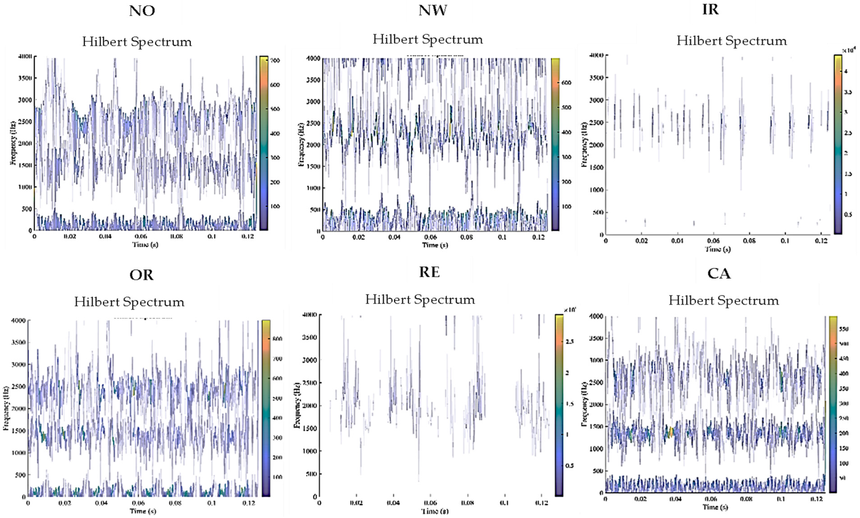
4.3. Hilbert–Huang Transform (HHT)

The HHT computes the instantaneous frequency of a time series signal $x\left(t\right)$, which reveals the intra-wave frequency modulations [104]. It can be defined by the complex conjugate $y\left(t\right)$ of the targeted time series signal $x\left(t\right)$ such that

$$y\left(t\right)=\frac{P}{\pi } {{\displaystyle \int }}_{-\infty }^{+\infty }\frac{x\left(\tau \right)}{t-\tau } d\tau$$

(31)

Here, $P$ represents the principal value of the singular integral. The instantaneous frequency $w\left(t\right)$ is the time derivative of the instantaneous phase $\phi \left(t\right)$ such that

$$\phi \left(t\right)=\arctan \left(\frac{y\left(t\right)}{x\left(t\right)}\right)$$

(32)

$$w\left(t\right)=\frac{d\phi \left(t\right)}{dt}$$

(33)

Two simple ways to perform the HHT are: (1) by transforming the time series $x\left(t\right)$ into the frequency domain using FFT, shifting the phase angle of all the signal components, and then transforming back to the time domain; (2) by decomposing the time series signal into intrinsic mode functions (IMFs) using the empirical mode decomposition (EMD) or variational mode decomposition (VMD) techniques and then performing the HT [105,106,107]. Figure 22 and Figure 23 show examples of the produced Hilbert spectrums using HHT with EMD and VMD, respectively, from the bearing vibration signals with the six health conditions that were described in Section 2.1.1 above.

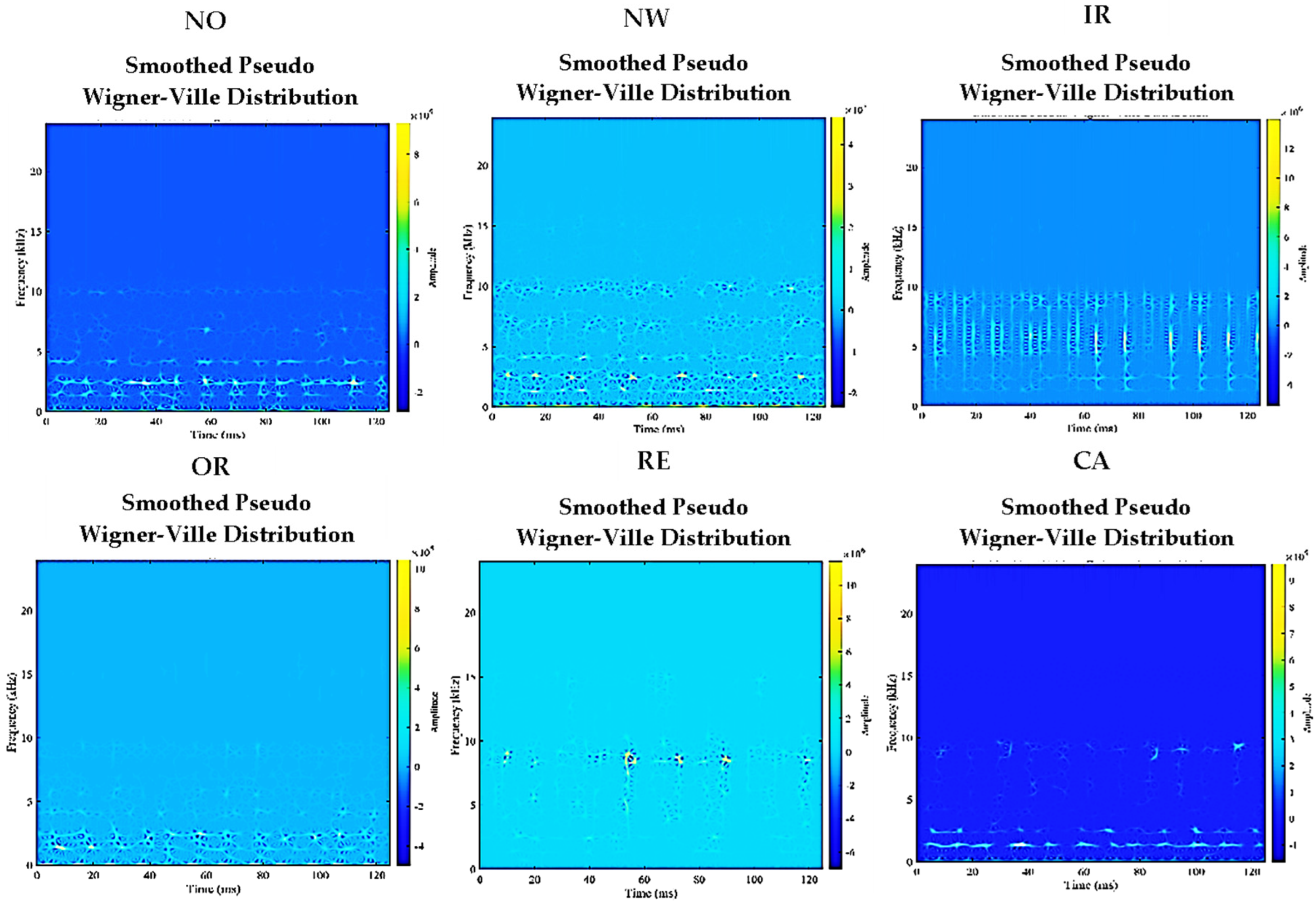
4.4. Wigner–Ville Distribution (WVD)

The WVD is achieved by simplifying the relationship between the power spectrum and the autocorrelation function for a non-stationary, time-variant process [108,109]. It has been used in signal visualisation, detection, and estimation. The WVD can be defined mathematically using the following equation

$$W\left(t,f\right)={\mathcal{F}}_{\tau \to f} \left\{z\left(t+\frac{\tau }{2} \right)z^{\ast }\left(t-\frac{\tau }{2} \right)\right\}$$

(34)

Here, $z$ is the analytic signal of $x\left(t\right)$ and can be computed as follows

$$z\left(t\right)=x\left(t\right)+j\widehat{x}\left(t\right)$$

(35)

where $\widehat{x}\left(t\right)$ is the Hilbert transform of $x\left(t\right)$. The WVD requires sharpening as it often contains some interference. One may use a lowpass windows filter to sharpen the distribution. Figure 24 presents examples of the computed smoothed pseudo WVD of the bearing vibration signals with the six different health conditions.

4.5. Variational Mode Decomposition (VMD)

The basic idea of VMD is to decompose the input signal into a discrete number of sub-modes, which have particular sparsity properties [106,110,111]. The bandwidth of each mode is selected to be the sparsity prior in the spectral domain. As described in [106], the bandwidth of a mode can be assessed using the following steps:

• Compute the analytic signal using HHT.
• Shift the mode’s frequency spectrum to the baseband.
• Estimate the bandwidth using the $H^1$ Gaussian smoothness of the demodulated signal.

The solution can be described as a constrained variation problem such that

$$\begin{array}{c}min\\ \left\{u_k\right\},\left\{w_k\right\}\end{array}\left\{{{\displaystyle \sum }}_k||{\partial }_t[(\delta \left(t\right)+\frac{j}{\pi t})\times u_k\left(t\right)e^{-j{w}_{k}t}||\begin{array}{c}2\\ 2\end{array}\right\} subject to {{\displaystyle \sum }}_k{u}_k=f$$

(36)

Here, $u_k$ is the set of all modes, $w_k$ is the set of their corresponding center pulsation, ${\partial }_t$ is the first-order partial derivative, and $\delta \left(t\right)$ is the average pulse function. Next, there is the augmented Lagrangian $\mathcal{L}$ such that

$$\begin{gathered} \mathcal{L}(\left\{u_k\right\},\left\{w_k\right\}≔ \alpha {{\displaystyle \sum }}_k||{\partial }_t[(\delta \left(t\right)+\frac{j}{\pi t})\times u_k\left(t\right)]e^{-j{w}_{k}t}||\begin{array}{c}2\\ 2\end{array}+ \\ \Vert f\left(t\right)-{{\displaystyle \sum }}_k{u}_k\left(t\right)\Vert \begin{array}{c}2\\ 2\end{array}+\langle \lambda \left(t\right), f\left(t\right)-{{\displaystyle \sum }}_k{u}_k\left(t\right)\rangle \end{gathered}$$

(37)

Here, α is the secondary penalty factor and $\lambda \left(t\right)$ represents the Lagrangian multiplication operator. As described in [106,112,113,114], Equation (37) can be solved using an alternate direction method of multipliers (ADMM). Those readers who are interested in more details of the mathematical formulation of VMD may be referred to [106,112]. Several studies have assessed the efficacy of VMD in machine fault diagnosis [113,114,115,116].

4.6. Stockwell Transform (ST)

The Stockwell transform (ST) is a time-frequency domain decomposition transform [117]. It is like a fusion between the Gabor transform and the WT [118]. Figure 25 presents examples of the ST-based computed images of the bearing vibration signals with the six different health conditions that were described in Section 2.1.1 above. In [118], the authors considered the application of ST in bearing fault diagnosis where the discrete orthonormal ST (DOST) is employed to form 2D images with identical patterns from the original vibration signals. Then, a CNN is used to perform the feature learning and classification tasks.

4.7. Multi-Domain Fusion Vibration Imaging (MDFVI)

In this technique, the features of the vibration images are considered in three domains of analysis, namely the time domain, frequency domain, and time-frequency domain, to generalise the feature space of the vibration-based health condition. In [119], each type of feature information from the three considered domains, i.e., the time, frequency, and time-frequency domains, is first converted into a 2D image, directly from the vibration signal, using FFT and envelop analysis, respectively. Then, the produced 2D images are converted into grayscale images that are combined to produce the MDFVI images. Finally, the MDFVI images are employed as inputs into a multitask learning (MTL)-based CNN architecture to perform the fault identification task. Dong et al. [120] proposed multi-stream CNNs for rotating machinery fault diagnosis. In this technique, four input types, including time domain, frequency domain, STFT-based time-frequency, and WT-based time–frequency inputs. Then, transfer learning-based CNN with VGG16, ResNet18, and ResNet34 was used to train models for machinery fault diagnosis.

5. Conclusions

Computer vision is one of the artificial intelligence applications that can observe and extract useful information from images and videos. Techniques that are able to observe, extract, and produce features from images and videos represent the basis of various innovations in digital healthcare and autonomous and smart manufacturing. These include image and video processing, object detection and segmentation, and image classification. In the field of machine fault diagnosis, an increased interest in converting the 1D vibration signal into a 2D image, which often offers discriminative features of the vibration signal, has emerged from recent advances in the field of computer vision.

In this review, we have attempted to bring together various techniques that produce vibration image representations from the time series vibration signals in one place. Different methods have been proposed to produce vibration image representations by encoding the time series vibration signals enabling the use of techniques from computer vision for machine fault diagnosis. A considerable amount of literature has been published on 2D vibration image representations produced in the time domain, frequency domain, and time-frequency domain for machine fault diagnosis. These techniques can be used individually or in combination to convert the 1D vibration signal into a 2D vibration image.

Table 1. Summary of the time domain vibration image representation techniques that are used in different studies of machine fault diagnosis.

Ref	VIR Technique	Feature Learning and Classification Method	RM Component	Dataset	Best Test Accuracies (%)
[36]	RGBVI	CNN	Bearing	f = 12 kHz and 48 kHz classes = 10 loads = 3 CWRU BDC Link https://engineering.case.edu/bearingdatacenter/download-data-file (accessed on 18 November 2022)	100 99.9
[47]	Grayscale image	CNN	Bearing	f = 12 kHz classes = 10 loads = 3 CWRU BDC Link https://engineering.case.edu/bearingdatacenter/download-data-file (accessed on 18 November 2022)	99.95 98.17
[48]	Grayscale image + LBP	RF, k-NN, naive Bayes, Bayes net, ANN	Bearing	f = 24 kHz classes = 3	100
[49]	Grayscale image + DNS	SVM	Motor faults	classes = 88	100
[50]	Grayscale image	WGAN-GP + SECNN	Bearing	f = 12 kHz classes = 10 loads = 3 CWRU BDC Link https://engineering.case.edu/bearingdatacenter/download-data-file (accessed on 18 November 2022)	99.6
[51]	Rectified signal + LBP	k-NN	Bearing	f = 12 kHz classes = 4 loads = 4 CWRU BDC Link https://engineering.case.edu/bearingdatacenter/download-data-file (accessed on 18 November 2022)	100
[53]	Multi-sensor data fusion	MB-CNN	Bearing and Gear	-	99.47
[55]	GAF MTF RP	CNN	Flight test helicopters Vibration measurements	f = 1.024 kHz classes = 2 Airbus SAS 2018 Link https://www.research-collection.ethz.ch/handle/20.500.11850/415151 (accessed on 18 November 2022)
[56]	GAF MTF	Capsule networks		f = 12 kHz f = 48 kHz classes = 4 CWRU BDC Link https://engineering.case.edu/bearingdatacenter/download-data-file (accessed on 18 November 2022)	99.81 99.51
[57]	MTF	ResNet CNN		f = 12 kHz classes = 10 CWRU BDC Link https://engineering.case.edu/bearingdatacenter/download-data-file (accessed on 18 November 2022)	98.5
[61]	HVI HOVI	Two-layer AdaBoost	AMB–rotor system	f = 25 kHz classes = 4	79.5 84.4
[62]	HOVI SDA PSDA	MSVM	Gearbox	f = 50 kHz classes = 10 loads = 3	99.2 99.78
[63]	Probability plot	Absolute value principal component analysis (AVPCA)	Bearing	f = 17.06 kHz classes = 3	98.22

VIR = vibration image representations; ML = machine learning; RM = rotating machine, CWRU BDC = Case Western Reserve University Bearing Data Center; k-NN = k-nearest neighbour classifier; MB-CNN = multi-sensor data fusion and bottleneck layer optimized convolutional neural network; RF = random forest; ANN = artificial neural network; WGAN-GP = Wasserstein generative adversarial network with gradient penalty; SECNN = self-attentive CNN.

summarises some of the studies that used vibration image representations produced in the time domain. As can be seen in Table 1, with different vibration datasets, most of the listed techniques achieve high classification accuracies (above 99%), while HVI and HOVI with two-layer AdaBoost achieved low classification accuracies of 79.5% and 84.4%, respectively, when used individually. In combination with SDA and PSDA, HOVI can achieve a classification accuracy of 99% and above.

Table 2. Summary of the frequency domain vibration image representation techniques that are used in different studies of machine fault diagnosis.

Ref	VIR Technique	ML Technique	RM Component	Dataset	Best Test Accuracies (%)
[69]	The FFT spectrum image	Minimum distance criterion based on the Eigen images	Bearing	classes = 4 loads = 4 CWRU BDC Link https://engineering.case.edu/bearingdatacenter/download-data-file (accessed on 18 November 2022)	100
[72]	The FFT spectrum image	CNN	Bearing	f = 12 kHz classes = 12 CWRU BDC Link https://engineering.case.edu/bearingdatacenter/download-data-file (accessed on 18 November 2022)	99.5
[73]	The FFT spectrum image based on segmented time series signal	ANN	Bearing	f = 12 kHz classes = 4 CWRU BDC Link https://engineering.case.edu/bearingdatacenter/download-data-file (accessed on 18 November 2022)	100
[74]	The FFT spectrum image based on a segmented time series signal	CNN	Bearing	f = 25.6 kHz classes = 5 Unit of research in advanced materials (URMA)   f = 48 kHz classes = 10 CWRU BDC Link https://engineering.case.edu/bearingdatacenter/download-data-file (accessed on 18 November 2022)	100           99.68
[75]	The FFT spectrum image	ANN	Fan	f = 1.6 kHz classes = 4	99.01
[76]	Adjusted FFT Spectrum Image	2DPCA + NNC	Bearing	f = 12 kHz classes = 4 loads = 4 CWRU BDC Link https://engineering.case.edu/bearingdatacenter/download-data-file (accessed on 18 November 2022)	100
[80]	Image representations using bi-spectrum	Probabilistic neural network PNN	Axial piston hydraulic pump and Self-priming centrifugal pumps	f = 10.239 kHz classes = 5     f = 1 kHz classes = 3	98.33       98.71

presents a summary of some studies that used vibration image representations produced in the frequency domain. The FFT spectrum achieved high classification accuracy in different case studies. In addition,

Table 3. Summary of the time-frequency domain vibration image representation techniques that are used in different studies of machine fault diagnosis.

Ref	VIR Technique	ML Technique	RM Component	Dataset	Best Test Accuracies (%)
[82]	The STFT spectrogram image	CNN-AE	Rotary system	classes = 5 loads = 4 f = 12 kHz	99.8
[83]	The STFT spectrogram image	CNN based on a capsule network with an inception block (ICN)	Bearing	f = 48 kHz loads = 3 CWRU BDC Link https://engineering.case.edu/bearingdatacenter/download-data-file (accessed on 18 November 2022) and f = 64 kHz loads = 3 Paderborn University, Faculty of Mechanical Engineering https://mb.uni-paderborn.de/en/kat/main-research/datacenter/bearing-datacenter/data-sets-and-download (accessed on 18 November 2022)	97.15
[84]	The STFT spectrogram image	CNN using the scaled exponential linear unit (SELU) and hierarchical regularization	Bearing	f = 12 kHz classes = 10 CWRU BDC Link https://engineering.case.edu/bearingdatacenter/download-data-file (accessed on 18 November 2022) and f = 12.8 kHz Classes = 4 Yanshan University, Qinhuangdao, Hebei 066004, P. R. China. Bearings dataset collected from a mechanical vibration simulator	100         97.81
[85]	The STFT spectrogram image	Image classification transformer (ICT)	Bearing	f = 12 kHz classes = 4 loads = 4 CWRU BDC Link https://engineering.case.edu/bearingdatacenter/download-data-file (accessed on 18 November 2022)	98.3
[86]	The STFT spectrogram image	CNN	Bearing	f = 97.6 and 48.8 kHz classes = 3 MFPT Link https://www.mfpt.org/fault-data-sets/ (accessed on 18 November 2022)	94.99
[87]	The STFT spectrogram image	DCNN	High-speed milling machine	f = 50 kHz milling cutters = 3
[88]	The STFT spectrogram image	2DCNN	Bearing and Tool wear	f = 12 kHz classes = 4 CWRU BDC Link https://engineering.case.edu/bearingdatacenter/download-data-file (accessed on 18 November 2022) and f = 100 kHz classes = 2	100       100
[89]	The Grad-CAM activation maps for STFT-based images	CNN	Bearing	f = 12 kHz classes = 12 CWRU BDC Link https://engineering.case.edu/bearingdatacenter/download-data-file (accessed on 18 November 2022) and f = 100 kHz classes = 7	96.9     88
[91]	The Grad-CAM activation maps for STFT-based images	CNN NN ANFIS	Bearing	f = 12 kHz classes = 4 CWRU BDC Link https://engineering.case.edu/bearingdatacenter/download-data-file (accessed on 18 November 2022)	100 100 96.9
[93]	Order maps	CNN	Locomotive rolling element bearings	f = 25.6 kHz classes = 3 and f = 20 kHz classes = 5	98.4     98.6
[100]	CWT	RDPN-FCDAE	Bearing	f = 20 kHz classes = 9	98.28
[101]	CWT	CNN with LeNet-5 and RF	Bearing	f = 12 kHz classes = 10 CWRU BDC Link https://engineering.case.edu/bearingdatacenter/download-data-file (accessed on 18 November 2022) and f = 20 kHz classes = 4 Tongji University	99.73       97.38
[102]	CWT	CNN	Hydraulic axial piston pump	f = 24.5 kHz classes = 5	98.44
[103]	Grayscale image + Scalogram	DNN	Bearing	f = 12 kHz classes = 10 CWRU BDC Link https://engineering.case.edu/bearingdatacenter/download-data-file (accessed on 18 November 2022)	100
[107]	STFT WT HHT	CNN	Bearing	f = 97.6 classes = 3 MFPT Link https://www.mfpt.org/fault-data-sets/ (accessed on 18 November 2022)	91.7 99.9 91.7
[109]	WVD	ANN	Bearing	-	-
[113]	VMD	DenseNet	Bearing	f = 200 kHz classes = 5 University of Ottawa Link https://data.mendeley.com/datasets/v43hmbwxpm/2 (accessed on 18 November 2022)	92.0
[114]	VMD	ResNet 101	Motor	f = 51.2 kHz classes = 6 the Federal University of Rio de Janeiro Link https://www02.smt.ufrj.br/~offshore/mfs/page_01.html#SEC2 (accessed on 18 November 2022)	94.0
[115]	VMD	CNN	Planetary Gear	f = 12.8 kHz classes = 4 Spectra Quest Company	98.75
[116]	VMD	DNN	Rail serviced vehicle	f = 12.8 kHz classes = 4	99.75
[118]	DOST	CNN	Bearing	f = 12 kHz classes = 6 CWRU BDC Link https://engineering.case.edu/bearingdatacenter/download-data-file (accessed on 18 November 2022)	99.8
[119]	MDFVI Multi-domain fusion of grayscale from raw data, FFT, and envelop analysis	MTL-CNN	Bearing	f = 65.536 kHz classes = 4 and f = 12 kHz classes = 4 CWRU BDC Link https://engineering.case.edu/bearingdatacenter/download-data-file (accessed on 18 November 2022)	100     100

shows a summary of some studies that used vibration image representations produced in the time–frequency domain. It has been demonstrated by these studies that 2D vibration image representations in the frequency domain and time–frequency domain are valuable and able to achieve high classification accuracies in different scenarios of machine fault diagnosis. The following conclusions and insights for future research can be drawn from the present review:

• The most obvious finding to emerge from the analysis in Table 1, Table 2 and Table 3 is that most of the listed techniques were able to achieve high classification accuracies.
• The machine fault diagnosis accuracies are likely to be related to how well the vibration image representations are produced using the various techniques described in this review and to how efficiently they are capable of divulging diverse forms of features for each machine health condition.
• The multi-domain fusion of information features from different domains can generalise the feature space of the vibration-based health condition, which makes it a promising technique to be used for producing vibration images from time series signals.
• The CNN deep learning architecture has been utilised in most of the studies, given its robust performance in image classification.
• Researchers have successfully employed various feature-learning and classification algorithms for fault classification using the produced vibration images. Of these, the deep learning techniques of the CNN-based pre-trained nets for transfer learning, such as ResNet, DenseNet, and LeNet-5, are promising in vibration image-based fault diagnosis. The CNNs have been used extensively with the produced vibration images for their reliability and validity in image classification. They are mainly beneficial for finding patterns in the produced vibration images for detection and classification tasks.
• For further improvement in the performance of CNNs in vibration-based fault diagnosis, future research into the regularization parameters, improvement of the activation functions, development of new loss functions, and construction of new CNN-based network structures will be helpful.
• Based on the successful application of some CNN-based pre-trained nets such as DenseNet future research might explore the use of recent developments in deep network architectures, such as RegNet [121], EfficientNet [122], and MobileNet [123].
• In most of these studies, the classification accuracy was considered and improved. However, other evaluation measures for the classification model need to be considered, such as recall, precision, F1 score, and ROC graphs.

Finally, in most of the introduced studies within these tables, links to their publicly available vibration datasets are provided.

References

- Ahmed, H.; Nandi, A.K. Condition Monitoring with Vibration Signals: Compressive Sampling and Learning Algorithms for Rotating Machines; John Wiley & Sons: Hoboken, NJ, USA, 2020. [Google Scholar]
- Ahmed, H.; Wong, M.; Nandi, A. Intelligent condition monitoring method for bearing faults from highly compressed measurements using sparse over-complete features. Mech. Syst. Signal Process. 2018, 99, 459–477. [Google Scholar] [CrossRef]
- Ahmed, H.O.A.; Nandi, A.K. Three-Stage Hybrid Fault Diagnosis for Rolling Bearings With Compressively Sampled Data and Subspace Learning Techniques. IEEE Trans. Ind. Electron. 2019, 66, 5516–5524. [Google Scholar] [CrossRef] [Green Version]
- Qu, Y.; He, D.; Yoon, J.; Van Hecke, B.; Bechhoefer, E.; Zhu, J. Gearbox Tooth Cut Fault Diagnostics Using Acoustic Emission and Vibration Sensors—A Comparative Study. Sensors 2014, 14, 1372–1393. [Google Scholar] [CrossRef] [PubMed]
- Azamfar, M.; Singh, J.; Bravo-Imaz, I.; Lee, J. Multisensor data fusion for gearbox fault diagnosis using 2-D convolutional neural network and motor current signature analysis. Mech. Syst. Signal Process. 2020, 144, 106861. [Google Scholar] [CrossRef]
- Resendiz-Ochoa, E.; Saucedo-Dorantes, J.J.; Benitez-Rangel, J.P.; Osornio-Rios, R.A.; Morales-Hernandez, L.A. Novel Methodology for Condition Monitoring of Gear Wear Using Supervised Learning and Infrared Thermography. Appl. Sci. 2020, 10, 506. [Google Scholar] [CrossRef] [Green Version]
- Ahmed, H.O.; Wong, M.D.; Nandi, A.K. Classification of bearing faults combining compressive sampling, laplacian score, and support vector machine. In Proceedings of the IECON 2017—43rd Annual Conference of the IEEE Industrial Electronics Society, Beijing, China, 29 October–1 November 2017; pp. 8053–8058. [Google Scholar]
- Ahmed, H.O.; Wong, M.D.; Nandi, A.K. Effects of deep neural network parameters on classification of bearing faults. In Proceedings of the IECON 2016—42nd Annual Conference of the IEEE Industrial Electronics Society 2016, Florence, Italy, 24–27 October 2016; pp. 6329–6334. [Google Scholar]
- Seera, M.; Wong, M.D.; Nandi, A.K. Classification of ball bearing faults using a hybrid intelligent model. Appl. Soft Comput. 2017, 57, 427–435. [Google Scholar] [CrossRef]
- Zhang, L.; Nandi, A.K. Fault classification using genetic programming. Mech. Syst. Signal Process. 2007, 21, 1273–1284. [Google Scholar] [CrossRef]
- Jack, L.B.; Nandi, A.K. Support vector machines for detection and characterization of rolling element bearing faults. Proc. Inst. Mech. Eng. Part C J. Mech. Eng. Sci. 2001, 215, 1065–1074. [Google Scholar] [CrossRef]
- Nayana, B.R.; Geethanjali, P. Analysis of Statistical Time-Domain Features Effectiveness in Identification of Bearing Faults From Vibration Signal. IEEE Sens. J. 2017, 17, 5618–5625. [Google Scholar] [CrossRef]
- Sreejith, B.; Verma, A.K.; Srividya, A. Fault diagnosis of rolling element bearing using time-domain features and neural networks. In Proceedings of the IEEE Region 10 and the Third International Conference on Industrial and Information Systems, Kharagpur, India, 8–10 December 2008; Volume 8, pp. 1–6. [Google Scholar]
- Bouguerriou, N.; Haritopoulos, M.; Capdessus, C.; Allam, L. Novel cyclostationarity-based blind source separation algorithm using second order statistical properties: Theory and application to the bearing defect diagnosis. Mech. Syst. Signal Process. 2005, 19, 1260–1281. [Google Scholar] [CrossRef]
- McCormick, A.C.; Nandi, A.K.; Jack, L.B. Application of periodic time-varying autoregressive models to the detection of bearing faults. Proc. Inst. Mech. Eng. Part C J. Mech. Eng. Sci. 1998, 212, 417–428. [Google Scholar] [CrossRef]
- McCormick, A.C.; Nandi, A.K. A comparison of artificial neural networks and other statistical methods for rotating machine condition classification. In Proceedings of the IEE Colloquium on Modeling and Signal Processing for Fault Diagnosis, IET, (Digest No: 1996/260), Leicester, UK, 18 September 1996. [Google Scholar]
- Guo, H.; Jack, L.; Nandi, A. Feature Generation Using Genetic Programming With Application to Fault Classification. IEEE Trans. Syst. Man Cybern. Part B (Cybern.) 2005, 35, 89–99. [Google Scholar] [CrossRef]
- Elasha, F.; Mba, D.; Ruiz-Carcel, C. A comparative study of adaptive filters in detecting a naturally degraded bearing within a gearbox. Case Stud. Mech. Syst. Signal Process. 2016, 3, 1–8. [Google Scholar] [CrossRef] [Green Version]
- Ahamed, N.; Pandya, Y.; Parey, A. Spur gear tooth root crack detection using time synchronous averaging under fluctuating speed. Measurement 2014, 52, 1–11. [Google Scholar] [CrossRef]
- Ayaz, E. Autoregressive modeling approach of vibration data for bearing fault diagnosis in electric motors. J. Vibroeng. 2014, 16, 2130–2138. [Google Scholar]
- Lin, H.-C.; Ye, Y.-C. Reviews of bearing vibration measurement using fast Fourier transform and enhanced fast Fourier transform algorithms. Adv. Mech. Eng. 2019, 11. [Google Scholar] [CrossRef]
- Farokhzad, S. Vibration Based Fault Detection of Centrifugal Pump by Fast Fourier Transform and Adaptive Neuro-Fuzzy Inference System. J. Mech. Eng. Technol. 2013, 82–87. [Google Scholar] [CrossRef]
- de Jesus Romero-Troncoso, R. Multirate signal processing to improve FFT-based analysis for detecting faults in induction motors. IEEE Trans. Ind. Inform. 2016, 13, 1291–1300. [Google Scholar] [CrossRef]
- McCormick, A.C.; Nandi, A.K. Real-time classification of rotating shaft loading conditions using artificial neural networks. IEEE Trans. Neural Netw. 1997, 8, 748–757. [Google Scholar] [CrossRef]
- Tian, J.; Morillo, C.; Azarian, M.H.; Pecht, M. Motor Bearing Fault Detection Using Spectral Kurtosis-Based Feature Extraction Coupled With K-Nearest Neighbor Distance Analysis. IEEE Trans. Ind. Electron. 2015, 63, 1793–1803. [Google Scholar] [CrossRef]
- Ahmed, H.; Nandi, A.K. Compressive Sampling and Feature Ranking Framework for Bearing Fault Classification With Vibration Signals. IEEE Access 2018, 6, 44731–44746. [Google Scholar] [CrossRef]
- Wang, Y.; Xiang, J.; Markert, R.; Liang, M. Spectral kurtosis for fault detection, diagnosis and prognostics of rotating machines: A review with applications. Mech. Syst. Signal Process. 2016, 66, 679–698. [Google Scholar] [CrossRef]
- Shakya, P.; Darpe, A.K.; Kulkarni, M.S. Vibration-based fault diagnosis in rolling element bearings: Ranking of various time, frequency and time-frequency domain data-based damage identi cation parameters. Int. J. Cond. Monit. 2013, 3, 53–62. [Google Scholar] [CrossRef]
- Wang, H.; Chen, P. Fuzzy Diagnosis Method for Rotating Machinery in Variable Rotating Speed. IEEE Sens. J. 2010, 11, 23–34. [Google Scholar] [CrossRef]
- Wang, L.; Liu, Z.; Miao, Q.; Zhang, X. Time–frequency analysis based on ensemble local mean decomposition and fast kurtogram for rotating machinery fault diagnosis. Mech. Syst. Signal Process. 2018, 103, 60–75. [Google Scholar] [CrossRef]
- Yu, J.; Lv, J. Weak Fault Feature Extraction of Rolling Bearings Using Local Mean Decomposition-Based Multilayer Hybrid Denoising. IEEE Trans. Instrum. Meas. 2017, 66, 3148–3159. [Google Scholar] [CrossRef]
- Halim, E.B.; Shah, S.L.; Zuo, M.J.; Choudhury, M.S. Fault detection of gearbox from vibration signals using time-frequency domain averaging. In Proceedings of the American Control Conference, Minneapolis, MN, USA, 14–16 June 2006; pp. 1–6. [Google Scholar]
- Pandhare, V.; Singh, J.; Lee, J. Convolutional Neural Network Based Rolling-Element Bearing Fault Diagnosis for Naturally Occurring and Progressing Defects Using Time-Frequency Domain Features. In Proceedings of the 2019 Prognostics and System Health Management Conference (PHM-Paris), Paris, France, 2–5 May 2019; pp. 320–326. [Google Scholar]
- Staszewski, W.; Worden, K.; Tomlinson, G. Time–frequency analysis in gearbox fault detection using the wigner–ville distribution and pattern recognition. Mech. Syst. Signal Process. 1997, 11, 673–692. [Google Scholar] [CrossRef]
- Jia, F.; Lei, Y.; Lin, J.; Zhou, X.; Lu, N. Deep neural networks: A promising tool for fault characteristic mining and intelligent diagnosis of rotating machinery with massive data. Mech. Syst. Signal Process. 2016, 72–73, 303–315. [Google Scholar] [CrossRef]
- Ahmed, H.O.A.; Nandi, A.K. Connected Components-based Colour Image Representations of Vibrations for a Two-stage Fault Diagnosis of Roller Bearings Using Convolutional Neural Networks. Chin. J. Mech. Eng. 2021, 34, 1–21. [Google Scholar] [CrossRef]
- Lei, Y.; Yang, B.; Jiang, X.; Jia, F.; Li, N.; Nandi, A.K. Applications of machine learning to machine fault diagnosis: A review and roadmap. Mech. Syst. Signal Process. 2020, 138, 106587. [Google Scholar] [CrossRef]
- Garcia-Ramirez, A.G.; Morales-Hernandez, L.A.; Osornio-Rios, R.A.; Benitez-Rangel, J.P.; Garcia-Perez, A.; Romero-Troncoso, R.D.J. Fault detection in induction motors and the impact on the kinematic chain through thermographic analysis. Electr. Power Syst. Res. 2014, 114, 1–9. [Google Scholar] [CrossRef]
- Bagavathiappan, S.; Lahiri, B.; Saravanan, T.; Philip, J.; Jayakumar, T. Infrared thermography for condition monitoring—A review. Infrared Phys. Technol. 2013, 60, 35–55. [Google Scholar] [CrossRef]
- Osornio-Rios, R.A.; Antonino-Daviu, J.A.; de Jesus Romero-Troncoso, R. Recent Industrial Applications of Infrared Thermography: A Review. IEEE Trans. Ind. Inform. 2019, 15, 615–625. [Google Scholar] [CrossRef]
- Sun, H.X.; Zhang, Y.H.; Luo, F.L. Visual inspection of surface crack on labyrinth disc in aeroengine. Opt. Precis. Eng. 2009, 17, 1187–1195. [Google Scholar]
- Ravikumar, S.; Ramachandran, K.; Sugumaran, V. Machine learning approach for automated visual inspection of machine components. Expert Syst. Appl. 2011, 38, 3260–3266. [Google Scholar] [CrossRef]
- Chauhan, V.; Surgenor, B. A Comparative Study of Machine Vision Based Methods for Fault Detection in an Automated Assembly Machine. Procedia Manuf. 2015, 1, 416–428. [Google Scholar] [CrossRef] [Green Version]
- Liu, L.; Zhou, F.; He, Y. Vision-based fault inspection of small mechanical components for train safety. IET Intell. Transp. Syst. 2016, 10, 130–139. [Google Scholar] [CrossRef]
- Karakose, M.; Yaman, O.; Baygin, M.; Murat, K.; Akın, E. A New Computer Vision Based Method for Rail Track Detection and Fault Diagnosis in Railways. Int. J. Mech. Eng. Robot. Res. 2017, 6, 22–27. [Google Scholar] [CrossRef]
- Ren, Z.; Fang, F.; Yan, N.; Wu, Y. State of the art in defect detection based on machine vision. Int. J. Precis. Eng. Manuf.-Green Technol. 2021, 9, 661–691. [Google Scholar] [CrossRef]
- Zhang, W.; Peng, G.; Li, C. Bearings Fault Diagnosis Based on Convolutional Neural Networks with 2-D Representation of Vibration Signals as Input. MATEC Web Conf. 2017, 95, 13001. [Google Scholar] [CrossRef] [Green Version]
- Kaplan, K.; Kaya, Y.; Kuncan, M.; Minaz, M.R.; Ertunç, H.M. An improved feature extraction method using texture analysis with LBP for bearing fault diagnosis. Appl. Soft Comput. 2020, 87, 106019. [Google Scholar] [CrossRef]
- Uddin, J.; Kang, M.; Nguyen, D.V.; Kim, J.-M. Reliable Fault Classification of Induction Motors Using Texture Feature Extraction and a Multiclass Support Vector Machine. Math. Probl. Eng. 2014, 2014, 1–9. [Google Scholar] [CrossRef]
- Tang, H.; Gao, S.; Wang, L.; Li, X.; Li, B.; Pang, S. A Novel Intelligent Fault Diagnosis Method for Rolling Bearings Based on Wasserstein Generative Adversarial Network and Convolutional Neural Network under Unbalanced Dataset. Sensors 2021, 21, 6754. [Google Scholar] [CrossRef] [PubMed]
- Khan, S.A.; Kim, J.-M. Automated Bearing Fault Diagnosis Using 2D Analysis of Vibration Acceleration Signals under Variable Speed Conditions. Shock Vib. 2016, 2016, 1–11. [Google Scholar] [CrossRef] [Green Version]
- Guo, Z.; Zhang, L.; Zhang, D. A Completed Modeling of Local Binary Pattern Operator for Texture Classification. IEEE Trans. Image Process. 2010, 19, 1657–1663. [Google Scholar] [CrossRef] [Green Version]
- Wang, H.; Li, S.; Song, L.; Cui, L. A novel convolutional neural network based fault recognition method via image fusion of multi-vibration-signals. Comput. Ind. 2018, 105, 182–190. [Google Scholar] [CrossRef]
- Wang, Z.; Oates, T. Encoding time series as images for visual inspection and classification using tiled convolutional neural networks. In Proceedings of the Workshops at the Twenty-Ninth AAAI Conference on Artificial Intelligence 2015, Austin, TX, USA, 25–30 January 2015; pp. 1–7. [Google Scholar]
- Garcia, G.R.; Michau, G.; Ducoffe, M.; Gupta, J.S.; Fink, O. Time series to images: Monitoring the condition of industrial assets with deep learning image processing algorithms. arXiv 2020, arXiv:2005.07031. [Google Scholar]
- Han, B.; Zhang, H.; Sun, M.; Wu, F. A New Bearing Fault Diagnosis Method Based on Capsule Network and Markov Transition Field/Gramian Angular Field. Sensors 2021, 21, 7762. [Google Scholar] [CrossRef]
- Yan, J.; Kan, J.; Luo, H. Rolling Bearing Fault Diagnosis Based on Markov Transition Field and Residual Network. Sensors 2022, 22, 3936. [Google Scholar] [CrossRef]
- Jp, E. Recurrence plots of dynamical systems. Europhys. Lett. 1987, 5, 973–977. [Google Scholar]
- Souza, V.M.; Silva, D.F.; Batista, G.E. Extracting texture features for time series classification. In Proceedings of the 2014 22nd International Conference on Pattern Recognition IEEE, Stockholm, Sweden, 24–28 August 2014; pp. 1425–1430. [Google Scholar]
- Kecik, K.; Smagala, A.; Lyubitska, K. Ball Bearing Fault Diagnosis Using Recurrence Analysis. Materials 2022, 15, 5940. [Google Scholar] [CrossRef]
- Yan, X.; Sun, Z.; Zhao, J.; Shi, Z.; Zhang, C.-A. Fault Diagnosis of Active Magnetic Bearing–Rotor System via Vibration Images. Sensors 2019, 19, 244. [Google Scholar] [CrossRef] [Green Version]
- Medina, R.; Macancela, J.-C.; Lucero, P.; Cabrera, D.; Cerrada, M.; Sánchez, R.-V.; Vásquez, R.E. Vibration signal analysis using symbolic dynamics for gearbox fault diagnosis. Int. J. Adv. Manuf. Technol. 2019, 104, 2195–2214. [Google Scholar] [CrossRef]
- Hamadache, M.; Lee, D.; Mucchi, E.; Dalpiaz, G. Vibration-Based Bearing Fault Detection and Diagnosis via Image Recognition Technique Under Constant and Variable Speed Conditions. Appl. Sci. 2018, 8, 1392. [Google Scholar] [CrossRef]
- Pichler, K.; Ooijevaar, T.; Hesch, C.; Kastl, C.; Hammer, F. Data-driven vibration-based bearing fault diagnosis using non-steady-state training data. J. Sens. Sens. Syst. 2020, 9, 143–155. [Google Scholar] [CrossRef]
- Igba, J.; Alemzadeh, K.; Durugbo, C.; Eiriksson, E.T. Analysing RMS and peak values of vibration signals for condition monitoring of wind turbine gearboxes. Renew. Energy 2016, 91, 90–106. [Google Scholar] [CrossRef] [Green Version]
- Nagel, L.; Galeazzi, R.; Voigt, A.J.; Santos, I.F. Fault diagnosis of active magnetic bearings based on Gaussian GLRT detector. In Proceedings of the 2016 3rd Conference on Control and Fault-Tolerant Systems (SysTol), Barcelona, Spain, 7–9 September 2016; pp. 540–547. [Google Scholar] [CrossRef] [Green Version]
- Yip, L. Analysis and Modeling of Planetary Gearbox Vibration Data for Early Fault Detection; University of Toronto: Toronto, ON, Canada, 2011. [Google Scholar]
- Asnaashari, E.; Sinha, J.K. Crack detection in structures using deviation from normal distribution of measured vibration responses. J. Sound Vib. 2014, 333, 4139–4151. [Google Scholar] [CrossRef]
- Li, W.; Qiu, M.; Zhu, Z.; Wu, B.; Zhou, G. Bearing fault diagnosis based on spectrum images of vibration signals. Meas. Sci. Technol. 2016, 27, 035005. [Google Scholar] [CrossRef]
- Diniz, P.S.R.; da Silva, E.A.B.; Netto, S.L. Digital Signal Processing System Analysis and Design; Cambridge University Press: Cambridge, UK, 2010. [Google Scholar] [CrossRef]
- Cochran, W.T.; Cooley, J.W.; Favin, D.L.; Helms, H.D.; Kaenel, R.A.; Lang, W.W.; Maling, G.C.; Nelson, D.E.; Rader, C.M.; Welch, P.D. What is the fast Fourier transform? Proc. IEEE 1967, 55, 1664–1674. [Google Scholar] [CrossRef]
- Liang, P.; Deng, C.; Wu, J.; Yang, Z.; Zhu, J. Intelligent fault diagnosis of rolling element bearing based on convolutional neural network and frequency spectrograms. In Proceedings of the 2019 IEEE International Conference on Prognostics and Health Management (ICPHM), San Francisco, CA, USA, 17–20 June 2019; pp. 1–5. [Google Scholar] [CrossRef]
- Amar, M.; Gondal, I.; Wilson, C. Vibration Spectrum Imaging: A Novel Bearing Fault Classification Approach. IEEE Trans. Ind. Electron. 2014, 62, 494–502. [Google Scholar] [CrossRef]
- Youcef Khodja, A.; Guersi, N.; Saadi, M.N.; Boutasseta, N. Rolling element bearing fault diagnosis for rotating machinery using vibration spectrum imaging and convolutional neural networks. Int. J. Adv. Manuf. Technol. 2020, 106, 1737–1751. [Google Scholar] [CrossRef]
- Khanna, S.; Huang, G.; Qiao, L.; Pavlovich, P.A.; Tiwari, S. Research on fan vibration fault diagnosis based on image recognition. J. Vibroeng. 2021, 23, 1366–1382. [Google Scholar] [CrossRef]
- Qiu, M.; Li, W.; Zhu, Z.; Jiang, F.; Zhou, G. Fault Diagnosis of Bearings with Adjusted Vibration Spectrum Images. Shock Vib. 2018, 2018, 1–17. [Google Scholar] [CrossRef]
- Zhang, L.; Jack, L.B.; Nandi, A.K. Fault detection using genetic programming. Mech. Syst. Signal Process. 2005, 19, 271–289. [Google Scholar] [CrossRef]
- Nikias, C.; Mendel, J. Signal processing with higher-order spectra. IEEE Signal Process. Mag. 1993, 10, 10–37. [Google Scholar] [CrossRef]
- McCormick, A.C.; Nandi, A.K. Bispectral and trispectral features for machine condition diagnosis. IEE Proc.-Vis. Image Signal Process. 1999, 146, 229–234. [Google Scholar] [CrossRef]
- Lu, C.; Wang, Y.; Ragulskis, M.; Cheng, Y. Fault Diagnosis for Rotating Machinery: A Method based on Image Processing. PLoS ONE 2016, 11, e0164111. [Google Scholar] [CrossRef] [Green Version]
- Cohen, L. Time-Frequency Analysis; Prentice Hall: Hoboken, NJ, USA, 1995. [Google Scholar]
- Wu, H.; Huang, A.; Sutherland, J.W. Condition-Based Monitoring and Novel Fault Detection Based on Incremental Learning Applied to Rotary Systems. Procedia CIRP 2022, 105, 788–793. [Google Scholar] [CrossRef]
- Zhu, Z.; Peng, G.; Chen, Y.; Gao, H. A convolutional neural network based on a capsule network with strong generalization for bearing fault diagnosis. Neurocomputing 2019, 323, 62–75. [Google Scholar] [CrossRef]
- Zhang, Y.; Xing, K.; Bai, R.; Sun, D.; Meng, Z. An enhanced convolutional neural network for bearing fault diagnosis based on time–frequency image. Measurement 2020, 157, 107667. [Google Scholar] [CrossRef]
- Alexakos, C.; Karnavas, Y.; Drakaki, M.; Tziafettas, I. A Combined Short Time Fourier Transform and Image Classification Transformer Model for Rolling Element Bearings Fault Diagnosis in Electric Motors. Mach. Learn. Knowl. Extr. 2021, 3, 228–242. [Google Scholar] [CrossRef]
- Jian, B.-L.; Su, X.-Y.; Yau, H.-T. Bearing Fault Diagnosis Based on Chaotic Dynamic Errors in Key Components. IEEE Access 2021, 9, 53509–53517. [Google Scholar] [CrossRef]
- Huang, Z.; Zhu, J.; Lei, J.; Li, X.; Tian, F. Tool Wear Monitoring with Vibration Signals Based on Short-Time Fourier Transform and Deep Convolutional Neural Network in Milling. Math. Probl. Eng. 2021, 2021, 1–14. [Google Scholar] [CrossRef]
- Chen, H.-Y.; Lee, C.-H. Deep Learning Approach for Vibration Signals Applications. Sensors 2021, 21, 3929. [Google Scholar] [CrossRef]
- Liefstingh, M.; Taal, C.; Restrepo, S.E.; Azarfar, A. Interpretation of Deep Learning Models in Bearing Fault Diagnosis. In Proceedings of the Annual Conference of the PHM Society, Virtual, 29 November–2 December 2021; Volume 13, pp. 1–9. [Google Scholar]
- Selvaraju, R.R.; Cogswell, M.; Das, A.; Vedantam, R.; Parikh, D.; Batra, D. Grad-CAM: Visual Explanations from Deep Networks via Gradient-Based Localization. In Proceedings of the 2017 IEEE International Conference on Computer Vision (ICCV), Venice, Italy, 22–29 October 2017; pp. 618–626. [Google Scholar] [CrossRef] [Green Version]
- Chen, H.-Y.; Lee, C.-H. Vibration Signals Analysis by Explainable Artificial Intelligence (XAI) Approach: Application on Bearing Faults Diagnosis. IEEE Access 2020, 8, 134246–134256. [Google Scholar] [CrossRef]
- Iandola, F.N.; Han, S.; Moskewicz, M.W.; Ashraf, K.; Dally, W.J.; Keutzer, K. SqueezeNet: AlexNet-level accuracy with 50x fewer parameters and< 0.5 MB model size. arXiv 2016, arXiv:1602.07360. [Google Scholar]
- Tayyab, S.M.; Chatterton, S.; Pennacchi, P. Intelligent Defect Diagnosis of Rolling Element Bearings under Variable Operating Conditions Using Convolutional Neural Network and Order Maps. Sensors 2022, 22, 2026. [Google Scholar] [CrossRef]
- Daubechies, I. The wavelet transform, time-frequency localization and signal analysis. IEEE Trans. Inf. Theory 1990, 36, 961–1005. [Google Scholar] [CrossRef] [Green Version]
- Burrus, C.S.; Gopinath, R.A.; Guo, H.; Odegard, J.E.; Selesnick, I.W. Introduction to Wavelets and Wavelet Transforms a Primer; Prentice Hall: Hoboken, NJ, USA, 1998; Volume 1. [Google Scholar]
- Saxena, M.; Bannet, O.O.; Gupta, M.; Rajoria, R. Bearing Fault Monitoring Using CWT Based Vibration Signature. Procedia Eng. 2016, 144, 234–241. [Google Scholar] [CrossRef] [Green Version]
- Mallat, S.G. A theory for multiresolution signal decomposition: The wavelet representation. IEEE Trans. Pattern Anal. Mach. Intell. 1989, 11, 674–693. [Google Scholar] [CrossRef] [Green Version]
- Mertins, A.; Mertins, D.A. Signal Analysis: Wavelets, Filter Banks, Time-Frequency Transforms and Applications; John Wiley & Sons, Inc.: Hoboken, NJ, USA, 1999. [Google Scholar]
- Shen, C.; Wang, D.; Kong, F.; Tse, P.W. Fault diagnosis of rotating machinery based on the statistical parameters of wavelet packet paving and a generic support vector regressive classifier. Measurement 2013, 46, 1551–1564. [Google Scholar] [CrossRef]
- Shi, H.; Chen, J.; Si, J.; Zheng, C. Fault Diagnosis of Rolling Bearings Based on a Residual Dilated Pyramid Network and Full Convolutional Denoising Autoencoder. Sensors 2020, 20, 5734. [Google Scholar] [CrossRef] [PubMed]
- Xu, G.; Liu, M.; Jiang, Z.; Söffker, D.; Shen, W. Bearing Fault Diagnosis Method Based on Deep Convolutional Neural Network and Random Forest Ensemble Learning. Sensors 2019, 19, 1088. [Google Scholar] [CrossRef] [PubMed] [Green Version]
- Tang, S.; Yuan, S.; Zhu, Y.; Li, G. An Integrated Deep Learning Method towards Fault Diagnosis of Hydraulic Axial Piston Pump. Sensors 2020, 20, 6576. [Google Scholar] [CrossRef] [PubMed]
- Nguyen, V.-C.; Hoang, D.-T.; Tran, X.-T.; Van, M.; Kang, H.-J. A Bearing Fault Diagnosis Method Using Multi-Branch Deep Neural Network. Machines 2021, 9, 345. [Google Scholar] [CrossRef]
- Huang, N.E. Hilbert-Huang Transform and Its Applications; World Scientific: Singapore, 2014. [Google Scholar]
- Wu, Z.; Huang, N.E. Ensemble empirical mode decomposition: A noise-assisted data analysis method. Adv. Adapt. Data Anal. 2009, 1, 1–41. [Google Scholar] [CrossRef]
- Dragomiretskiy, K.; Zosso, D. Variational mode decomposition. IEEE Trans. Signal Process. 2013, 62, 531–544. [Google Scholar] [CrossRef]
- Verstraete, D.; Ferrada, A.; Droguett, E.L.; Meruane, V.; Modarres, M. Deep Learning Enabled Fault Diagnosis Using Time-Frequency Image Analysis of Rolling Element Bearings. Shock Vib. 2017, 2017, 5067651. [Google Scholar] [CrossRef] [Green Version]
- Wigner, E. On the Quantum Correction For Thermodynamic Equilibrium. Phys. Rev. 1932, 40, 749–759. [Google Scholar] [CrossRef]
- Singru, P.; Krishnakumar, V.; Natarajan, D.; Raizada, A. Bearing failure prediction using Wigner-Ville distribution, modified Poincare mapping and fast Fourier transform. J. Vibroeng. 2018, 20, 127–137. [Google Scholar] [CrossRef] [Green Version]
- Wang, Q.; Wang, L.; Yu, H.; Wang, D.; Nandi, A.K. Utilizing SVD and VMD for Denoising Non-Stationary Signals of Roller Bearings. Sensors 2021, 22, 195. [Google Scholar] [CrossRef]
- Wang, Q.; Yang, C.; Wan, H.; Deng, D.; Nandi, A.K. Bearing fault diagnosis based on optimized variational mode decomposition and 1D convolutional neural networks. Meas. Sci. Technol. 2021, 32, 104007. [Google Scholar] [CrossRef]
- ur Rehman, N.; Aftab, H. Multivariate variational mode decomposition. IEEE Trans. Signal Process. 2019, 67, 6039–6052. [Google Scholar] [CrossRef] [Green Version]
- Lin, S.L. Intelligent fault diagnosis and forecast of time-varying bearing based on deep learning VMD-DenseNet. Sensors 2021, 21, 7467. [Google Scholar] [CrossRef]
- Lin, S.-L. Application Combining VMD and ResNet101 in Intelligent Diagnosis of Motor Faults. Sensors 2021, 21, 6065. [Google Scholar] [CrossRef]
- Li, Y.; Cheng, G.; Pang, Y.; Kuai, M. Planetary Gear Fault Diagnosis via Feature Image Extraction Based on Multi Central Frequencies and Vibration Signal Frequency Spectrum. Sensors 2018, 18, 1735. [Google Scholar] [CrossRef] [Green Version]
- Zheng, S.; Zhong, Q.; Chen, X.; Peng, L.; Cui, G. The Rail Surface Defects Recognition via Operating Service Rail Vehicle Vibrations. Machines 2022, 10, 796. [Google Scholar] [CrossRef]
- Wang, Y.; Orchard, J. Fast Discrete Orthonormal Stockwell Transform. SIAM J. Sci. Comput. 2009, 31, 4000–4012. [Google Scholar] [CrossRef]
- Hasan, M.J.; Kim, J.M. Bearing fault diagnosis under variable rotational speeds using stockwell transform-based vibration imaging and transfer learning. Appl. Sci. 2018, 8, 2357. [Google Scholar] [CrossRef] [Green Version]
- Hasan, J.; Islam, M.M.M.; Kim, J.-M. Bearing Fault Diagnosis Using Multidomain Fusion-Based Vibration Imaging and Multitask Learning. Sensors 2021, 22, 56. [Google Scholar] [CrossRef]
- Dong, H.; Lu, J.; Han, Y. Multi-Stream Convolutional Neural Networks for Rotating Machinery Fault Diagnosis under Noise and Trend Items. Sensors 2022, 22, 2720. [Google Scholar] [CrossRef] [PubMed]
- Radosavovic, I.; Kosaraju, R.P.; Girshick, R.; He, K.; Dollár, P. Designing network design spaces. In Proceedings of the IEEE/CVF Conference on Computer Vision and Pattern Recognition 2020, Seattle, WA, USA, 13–19 June 2020; pp. 10428–10436. [Google Scholar]
- Tan, M.; Le, Q. Efficientnet: Rethinking model scaling for convolutional neural networks. In Proceedings of the International Conference on Machine Learning 2019, Long Beach, CA, USA, 9–15 June 2019; pp. 6105–6114. [Google Scholar]
- Howard, A.; Sandler, M.; Chu, G.; Chen, L.C.; Chen, B.; Tan, M.; Wang, W.; Zhu, Y.; Pang, R.; Vasudevan, V.; et al. Searching for mobilenetv3. In Proceedings of the IEEE/CVF International Conference on Computer Vision 2019, Seoul, Republic of Korea, 27–28 October 2019; pp. 1314–1324. [Google Scholar]