Cooperative Adaptive Cruise Algorithm Based on Trajectory Prediction for Driverless Buses

Abstract

Cooperative adaptive cruise control (CACC) technology offers a proven solution to the current traffic congestion problems caused by the yearly growth of car ownership. Coping with random lane changes of bypass vehicles under the condition of traffic congestion is a challenge for urban driverless vehicles. In this paper, to meet the demand for high comfort driverless buses driving on urban roads, an active anti-disturbance following control method for driverless buses based on bystander vehicle intention recognition and trajectory prediction is proposed for the scenario of bystander vehicle cut-in during driving to alleviate the disturbance caused by bystander vehicles, improve passenger comfort, and suppress multi-vehicle oscillation. The simulation results show that the intelligent prediction system-based queue reduces the traffic oscillation rate by an average of 9.8% and improves the comfort level by an average of 11% under side-car insertion conditions. The results of the real vehicle test show that the vehicles based on the intelligent prediction algorithm have a 25.5% reduction in maximum speed adjustment, 14.5 m average reduction in following distance, 6% improvement in comfort, and 27% improvement in rear vehicle comfort.

1. Introduction and Related Research

1.1. Introduction

Most CACC algorithms consider only the traffic information at the current moment as input, and their performance may be limited under some complex operating conditions, for example, the side lane vehicles cut into the working conditions. It is thus highly desirable to use predictive algorithms that predict future driving conditions to achieve smoother speed control, thereby reducing traffic oscillations and passenger line comfort. Therefore, on this basis, this paper addresses the cut-in working conditions of the by-pass vehicles, by predicting the lane change intentions and trajectories of the by-pass vehicles, and flexing the following distance and speed in advance in order to improve passenger comfort and reduce the distance.

1.2. Related Research

CACC is the use of V2V communication technology in combination with the ACC system to ensure stable following of the queueing vehicles. Compared to ACC, CACC has more powerful collision avoidance and maximizes traffic flow throughput. CACC can improve traffic flow by reducing headway time distance and reducing traffic disturbance.

In the queueing truck for the CACC development at Auburn University [1], when a cut-in is detected, the CACC switches the target from the lead truck to the cut-in vehicle in order to create a larger spacing between the following truck and the cut-in vehicle. This process results in reduced fuel savings because it requires more work from the longitudinal controller, which is dangerous if the clearance is not wide enough when the vehicle cuts in, especially considering that an 80,000 lb. trailer requires 400 to 500 feet of stopping distance on the highway. Therefore, it is essential to anticipate the cut-in intentions of other drivers in advance. In addition, vehicles cutting in the queue can lead to changes in the vehicle queue structure; hence, it is necessary to design an appropriate CACC architecture for queue adjustment and compensation.

CACC systems are able to prevent possible collisions and maintain normal queueing to prevent vehicles from entering neighboring lanes, and different research institutions have addressed this problem from different aspects, e.g., reconfiguring the controller, reconfiguring the controller structure, visual recognition, predicting intentions, and communication.

Milanes et al. [2] designed a CACC string controller considering both V2V vehicles and non-V2V vehicles, which included a spacing off controller, and a spacing adjustment controller, which could handle bypass lane vehicle cut-in scenarios, but this method did not predict the intention or trajectory of cut-in scenarios. Liu et al. [3] artificially captured the previous vehicle in state differences under different lane change methods and designed a cost function for the head vehicle, while considering ride comfort and spacing safety on the basis of the free headway distance set ahead. This cost function integrated the trajectory differences of the insertion vehicle, making the controller sensitive to different lane change methods, and the results showed that the controller considering the differences in lane change behavior had smaller speed and spacing fluctuations when handling lane change perturbations. Han et al. [4] considered heterogeneous traffic composed of vehicles with different characteristics and formulated the longitudinal control problem as an output with a quadratic function tracking control problem, thus realizing the contradiction between different tracking requirements, including vehicle spacing, speed, and acceleration. In addition, the concepts of “expected speed” and “expected acceleration” were introduced to design the desired speed and acceleration to achieve additional goals and improve the predictive capability.

Liu et al. [5] improved the control structure of a typical original CACC system in order to improve the response of the system to the cut-in and cut-out of a vehicle in the bypass lane, and they designed a synthetic control structure that integrated a feed-forward control module with a conventional feedback CACC system. On the basis of the improved control structure, a variable acceleration limit (VAL) control algorithm was proposed, which was specifically applied to the feed-forward control model to suppress the propagation of oscillations in CACC due to vehicle cut-in in the side lane. Jun et al. [6] improved the spacing strategy of the CACC system, and the improved strategy could be used to predict the acceleration of the vehicle by means of workshop wireless communication to obtain the vehicle’s speed variation trend. The perspicacity and anti-interference performance of the distance control were improved.

Ko and Chang, from KAIST University, Korea Institute of Electrical Engineering [7], used the turn signal of the cut-in vehicle to create a virtual vehicle by recognizing the turn signal of the target vehicle ahead to avoid the effect of vehicle cut-in or cut-out conditions on the CACC system in advance, which can be applied to vehicles not equipped with communication devices or in areas with weak or nonexistent communication signals. The disadvantage is that this system is more affected by weather factors and driver personality and malfunction.

Kazemi et al. [8] built a subsystem of neural network-based driver behavior models for insertion prediction based on the inability of the CACC system to handle queue oscillations due to the insertion problem of vehicles in the side lane, and they designed a specific stochastic model predictive controller that incorporates this cut-in probability to enhance its response to detected dangerous cut-in maneuvers. Remmen et al. [9] used machine learning to predict vehicle cut-in maneuvers and selected different methods for behavior prediction including logistic regression, random forest classifier, support vector machine, and adaboost classifier; they averaged the outputs of the above models to create an integrated model. Douglass Jr et al. [10] used an ensemble LSTM-based deep neural network to perform multi-modal prediction of traffic vehicles around trucks in a simulated environment, classifying potential vehicle behavior as “passing” and “cut-in”. Gao et al. [11] proposed using the idea of reinforcement learning (RL), which does not rely on the accurate modeling of bus vehicle dynamics. Considering a time-varying topology, each autonomous vehicle received information only from previous vehicles within its communication range and learned the distributed controller in real time from online time–distance, velocity, and acceleration data collected from the system trajectory. Results showed that dedicated bus lane travel times were close to current travel times even with a 30% increase in transit capacity. Jurj et al. [12] trained the reviewer (SAC) reinforcement learning (RL) algorithm, which used physical knowledge, such as distances, to avoid interference, to automatically adjust the ideal longitudinal distance between the self and the leading vehicle. The physically guided (PG) RL method was better to avoid collisions in any selective deceleration condition and any queueing condition, and the method was more reliable.

The boundaries of several types of the control methods analyzed above are located in the controlled vehicle. Furthermore, with the advancement of 5G communication technology in recent years, shop floor communication and vehicle infrastructure communication have attracted increasing attention from researchers as a way to address the limitation of too short ACC fields of view.

Ploeg et al. [13] funded by the Dutch Ministry of Economic Affairs through the High-Tech Automotive Systems (HTAS) project, from the California Advanced Transportation and Freeway Partnership Program at the University of California, Berkeley, Institute of Transportation Studies, addressed the situation arising from special working conditions through the popularization of devices and the application of 5G communication. Such methods can guarantee short-range following, as well as string stability. Bosch, together with Huawei and Vodafone, the U.K. mobile network operator, demonstrated that direct, delay-free data exchange between vehicles can also improve the functionality of driver assistance systems such as ACC [14,15,16].

The contributions of this paper are summarized as follows: (1) Based on the convolutional social pool trajectory prediction architecture, the driver personality factor algorithm and the model and sampling short-term optimization algorithm are used as a means to improve the distribution of future trajectory points during the time domain of autonomous driving prediction and to reduce the trajectory error of vehicle prediction. (2) A single/multi-vehicle intelligent predictive adaptive cruise control system based on an immunity controller, a softening corrector, and a flexible fading corrector is used and outperforms the other method by simulation and experimental results in real vehicles.

The rest of this paper is structured as follows. In Section 2, a multi-vehicle collaborative following framework based on by-pass lane prediction is proposed and each module is explained in detail in different subsections. Test results and analysis of the proposed approach are discussed in Section 3. Finally, Section 4 concludes the paper.

2. Materials and Methods

Figure 1 shows the framework of the cooperative adaptive cruise system with intelligent prediction proposed in this paper, including the prediction module, flexible following factor corrector, self-anti-disturbance controller, and flexible fading corrector.

The prediction module combines two algorithms: data-driven trajectory prediction and prototype trajectory prediction algorithms. The data-driven algorithm includes two modules: the first for driver unpredictable elements and the second for social long-term and short-term memory neural network prediction, as shown in the upper part of Figure 1. The trajectory prototype-driven method contains a module for kinematics, trajectory matching, and trajectory sampling. In the figure social-LSTM is a long and short-term neural network considering social interaction properties, CTRA-model is a constant-turn-rate and acceleration model, and V2V is the communication between vehicles.

The flexible following factor corrector is the distribution degree of the road centerline which is then employed as the lane change overlap degree, and the flexible following factor and flexible switching factor of the following target are produced by a double second-order time-varying filter for flexible speed tracking after target switching. ${\mathsf{\rho }}_{\mathrm{flex}}$ is the flexible following factor in the speed control framework, and ${\mathsf{\tau }}_{\mathrm{flex}}$ flexibly switches the target switching factor _object at the time of target switching, preventing target switching when the switching factor is below a certain threshold. ${\mathrm{d}}_{\mathrm{obj}}$ and ${\mathrm{v}}_{\mathrm{obj}}$ are the speed and relative distance of the target vehicle.

The self-anti-disturbance controller, an instantaneous observation approach based on the expansion state observer, is proposed to correct for and suppress the internal disturbance generated by changes in the internal vehicle parameters and random disturbances induced by changes in the external road environment. The autonomous bus is finally directed to follow the target vehicle using an inverse longitudinal dynamics model that incorporates both a vehicle dynamics model and a motor-battery model. In the figure, ${\mathrm{a}}_{\mathrm{des}}$ is the expected acceleration, ${\mathrm{v}}_{\mathrm{act}-\mathrm{bus}1}$ is the actual velocity of vehicle 1, ${\mathrm{v}}_{\mathrm{act}-\mathrm{busi}}$ is the actual velocity of vehicle i, and ${\mathrm{T}}_{\mathrm{des}}$ and ${\mathrm{T}}_{\mathrm{br}\_\mathrm{des}}$ are the desired driving force and desired braking force of the vehicle.

The flexible attenuation corrector is a longitudinal following pattern correction for vehicles in the rear in response to bystander vehicles cutting into the open. ${\mathsf{\rho }}_{\mathrm{flex}-\mathrm{damp}}$ is the flexible attenuation following factor in the speed control framework.

2.1. Fusion Social-LSTM and Trajectory Prototype Prediction Algorithm

The prediction module is a vehicle trajectory dynamic prediction algorithm based on driving intention recognition, which provides the basis for the ACC and CACC of driverless buses during the process of vehicles cutting into the home lane from the side lane. First, a recurrent neural network model (Social-LSTM) based on social long-term and short-term memory is used as the base model of the trajectory dynamic prediction algorithm; then, a trajectory prototype is generated by setting a minimum value function to match the vehicle model with the planned sampled trajectory, and the trajectory prototype is used to modify the base prediction model to improve the correct rate of the short-term lane change trajectory prediction of the bypass vehicle. Finally, the driver adventurous factor is introduced into the driver’s lane change behavior character to further modify the base model and improve the correct rate of long-term lane change trajectory prediction of bypass vehicles.

$${\tau }_{character}=\frac{e^{-\frac{\alpha ·Agg+\beta Lan{e}_{ID}}{\omega ·T+\gamma ·Wi{d}_{vehicle}}}}{1+e^{-\frac{\alpha ·Agg+\beta Lan{e}_{ID}}{\omega ·T+\gamma ·Wi{d}_{vehicle}}}}$$

(1)

$$P_{predicted-driver}=P_{lanechange-fusion}\times {\tau }_{character}$$

(2)

$$T_{intention}\left(t\right)=\left[u_x,u_y,{\sigma }_x,{\sigma }_y,\rho \right]$$

(3)

$$Tra{j}_{model}=\tilde{x}\left(t+\Delta t\right)=\left(\begin{array}{c}x\left(t\right)\\ y\left(t\right)\\ \theta \left(t\right)\\ \dot{x}\left(t\right)\\ \ddot{x}\left(t\right)\\ \dot{\theta }\left(t\right)\end{array}\right)+\left(\begin{array}{l}\Delta x\left(t,\Delta t\right)\\ \Delta y\left(t,\Delta t\right)\\ \dot{\theta }\Delta t\\ \ddot{x}\Delta t\\ 0\\ 0\end{array}\right)$$

(4)

$$\left\{\begin{array}{c}S\left(x\right)=a_0+a_1{t}^1+a_2{t}^2+a_3{t}^3+a_4{t}^4+a_5{t}^5\\ S\left(y\right)=a_0+a_1{t}^1+a_2{t}^2+a_3{t}^3\end{array}\right.$$

(5)

$$Tra{j}_{sampling}\left(i\right)=S\left(t\right)$$

(6)

$$Tra{j}_{matching}=\frac{{{\displaystyle \sum }}_{i=0}^n\sqrt{\left(Tra{j}_{model}-Tra{j}_{sampling}\left(i\right)\right)}}{m}$$

(7)

$$T_{fusion}\left(t\right)={\omega }_{model}\times T_{model}\left(t\right)+{\omega }_{intention}\times T_{intention}\left(t\right)$$

(8)

where ${\tau }_{character}$ is the driver aggression factor, $P_{lanechange-fusion}$ is the social tensor input from the social pool layer, and $P_{predicted-driver}$ is the optimized social tensor. T is the headway time distance, and $\omega$ is the headway time distance as a percentage of the negative influence on the influence on the driver aggression factor. $Lan{e}_{ID}$ is the lane type, $\beta$ is the percentage of headway time distance to the positive influencing factor of driver aggressiveness. $Agg$ is the aggressiveness due to acceleration magnitude, and $\alpha$ is the percentage of acceleration/deceleration to the positive influencing factor of driver aggressiveness. $Wi{d}_{vehicle}$ is the model size, and γ is the percentage of the model with a negative influence on the driver adventurous factor. The $\alpha$, $\beta$, $\omega$, and γ parameters are assigned according to the probability of lane change. And $u_x,u_y,{\sigma }_x,{\sigma }_y,\rho$ are the five two-dimensional Gaussian distribution parameters based on the data-driven output. $T_{intention}$ is the trajectory of the data-driven output, $Tra{j}_{model}$ is the kinematic model, $Tra{j}_{sampling}$ is the trajectory sampling model, $Tra{j}_{matching}$ is the matching function of the kinematic model and trajectory sampling, $T_{fusion}$ is the fused trajectory, and ${\omega }_{model}$ and ${\omega }_{intention}$ are the trajectory prediction weights of different methods.

2.2. Flexible following Factor Corrector

On the basis of the anti-turbulence controller for speed following control, the flexibility corrector ensures the comfort of the driverless bus by softening the speed of the side lane vehicle with lane change intention and inserting it into the process of this lane. The flexibility corrector contains two parts: the flexibility correction factor and the following mode switching factor. The flexibility correction factor is calculated using the trajectory prediction results of the bypass lane vehicle in the lane change process (see Section 2.1), and the following mode switching factor uses the lane change intention of the bypass lane vehicle (see Section 2.1) as the switching condition of the following target. The intersection line between the vehicle and the lane centerline of the bypass lane vehicle during the lane change process shows Gaussian changes with the lane change process; hence, the process of the bypass lane vehicle passing the lane centerline is used as the criterion of the degree of the bypass lane vehicle covering this lane, i.e., the overlap degree between the bypass lane vehicle and the lane centerline is used as the flexible correction factor. The overlap degree under vehicle prediction, due to its additional spikes, cannot be directly used in the following mode; therefore, the flexible following factor is proposed. To calculate the flexible following factor, a dual second-order time-varying filter is selected. In the signal processing, the digital dual fourth-order filter is a second-order recursive linear filter containing two poles and two zeros.

$$Overlap\left(u_{x-lane},u_{y-lane}\right)=\frac{p_{lane}(x|\mu ,\Sigma )}{p_{max}(x|\mu ,\Sigma )}$$

(9)

$${\mathsf{\tau }}_{\mathrm{object}}={\mathsf{\rho }}_{\mathrm{flex}}=\mathrm{H}\left(z\right)=\frac{b_0+b_1{z}^{-1}+b_2{z}^{-2}}{a_0+a_1{z}^{-1}+a_2{z}^{-2}}$$

(10)

where $p_{lane}\left(x|\mu ,\Sigma \right)$ is the calculated value of the two-dimensional Gaussian distribution points under different positions of the vehicle, $Overlap$ is the overlap degree, ${\rho }_{flex} \mathrm{and} {\tau }_{object}$ are the flexible following factor and target switching factor, and $a_0,a_1,a_2,b_0,b_1,\mathrm{and} b_2$ are the curve change parameters, which are used as different parameters to ensure that the curve presents the change of the Gaussian curve, as well as the incremental change.

2.3. Self-Tampering Controller

The core control of speed control is the target vehicle speed following, and this subsection mainly establishes the control-oriented power system model and the inverse model based on the whole vehicle power transmission system. Among them, the whole vehicle dynamics model mainly includes the power source model, the power transmission system model, and the whole vehicle longitudinal dynamics model. In the conventional ACC system, the output of the lower controller in the hierarchical control, i.e., the input of the actuator, is the drive pedal opening and brake pedal opening transformed by the motor torque and brake pressure; thus, the role of the lower controller is to transform the output of the upper controller, i.e., the desired acceleration, into the input parameters of the actuator. In order to clearly express the input and output variables of the observer, the improved observer equation is as follows:

$$\left\{\begin{array}{l}\dot{z}=\left[A-LC\right]z+\left[B,L\right]u_c\\ y_c=z\end{array}\right.$$

(11)

where $u_c={[u y]}^T$ is the input variable of the observer, including the control quantity output by the control algorithm and the state variable output by the system. $y_c$ is the output of the observer, including the vehicle speed $v$, the first-order derivative of the vehicle speed $\dot{v}$, and the estimate of the disturbance $f$. After parameterization, the poles of the characteristic equation can be placed at the same position $\left(-{\omega }_o\right)$, and ${\omega }_o$ is the observer bandwidth, i.e., the gain matrix $L={[3{\omega }_0 3{{\omega }_0}^2 {{\omega }_0}^3]}^T$ of the observer is used.

2.4. Flexible Decay Algorithm

As shown in Figure 2, according to the analysis of the actual multi-vehicle following scenario, the impact of the speed change of the lead vehicle on the rear vehicle during the queue following process presents a weaker and weaker situation; therefore, the flexible attenuation factor of the queue following in this paper also presents a trend of smaller and smaller changes, i.e., the attenuation becomes smaller on the basis of the flexible factor of the lead vehicle to avoid the impact of the cut-in condition on the rear vehicle passenger comfort.

The variation in the state equation transformation function of the dual second-order time-varying filter is used to calculate the following flexible attenuation factor, while multiple spikes still exist in the late stage of the constructed function in the channel change, which cannot be logically switched; the factor is constructed as follows:

$${\mathsf{\tau }}_{{\mathrm{object}}_i}\left(\sigma \right)=\frac{0.2+0.3z^{-1}+0.2z^{-2}}{1-0.9z^{-1}+0.001z^{-2}}·{\alpha }_i$$

(12)

$${\mathsf{\rho }}_{{\mathrm{flex}}_i}\left(\sigma \right)=\frac{0.2+0.3z^{-1}+0.2z^{-2}}{1-z^{-1}+0.001z^{-2}}·{\beta }_i$$

(13)

where ${\alpha }_i$ and ${\beta }_i$ are the attenuation factors of the fleet; such parameters need to be constructed for different working conditions to verify their influence factors. To explore the laws of the two factors, different vehicle serial numbers and different speed ratios are constructed to explore the influence factors. The speed ratio is 0.83 for case 1 with a by-pass vehicle cut-in speed of 10 km/h and a queue vehicle speed of 14 km/h, and 0.85 for case 2 with a bypass vehicle cut-in speed of 12 km/h and a queue vehicle speed of 14 km/h. The results of the three simulations in Figure 3 show that the value of the attenuation factor needs to progressively decrease as the vehicle serial number increases, i.e., the impact of the cut-in vehicle on the vehicle influence becomes smaller and smaller. In Figure 4, the simulation results of different ranges of attenuation factors at different vehicle speeds show that, as the speed of the cut-in vehicle in the side lane approaches the speed ratio of the driverless bus queue vehicles, the value of the attenuation factor progressively decreases, i.e., if the speed of the cut-in vehicle is close to the speed of this lane, the attenuation factor is smaller.

The results of the above simulation show that the attenuation factor is related to the cut-in speed of the vehicle cutting into the side lane and the proximity to the speed of the train convoy, as well as the number of the team train (the head train number is 1, with numbers increasing in order); hence, the following function can be constructed:

$${\alpha }_i,{\beta }_i={\epsilon }_i=\mu ·\frac{1}{\raisebox{1ex}{$v_{side}$}\!\left/ \!\raisebox{-1ex}{$v_{queue}$}\right.}{e}^{-0.5{\left(\frac{i}{\raisebox{1ex}{$v_{side}$}\!\left/ \!\raisebox{-1ex}{$v_{queue}$}\right.}\right)}^2}$$

(14)

where $i$ is the queue train serial number, ${\epsilon }_i$ is the decay factor of queue train i, $\mu$ is the decay ratio (linearly increasing with the speed difference), $v_{side}$ is the speed of the side-car, and $v_i$ is the speed of queue train i.

Regarding safety, this paper defines a safety cost to evaluate the safety of the strategy, and the safety evaluation of vehicle $i$ at moment $k$ is shown in the following equation:

$$S{C}_i\left(k\right)=HW{T}_i\left(k\right)$$

(15)

where $HW{T}_i\left(k\right)$ is the headway time distance of vehicle k at moment i. This represents the time interval between the head ends of two consecutive vehicles passing through a certain section in a queue of vehicles traveling in the same lane. Regarding comfort, adopts jerk as the evaluation criterion of comfort, and its smaller value indicates the higher comfort level of the vehicle. However, for the queue vehicles, the following formula can be used to evaluate the comfort of the remaining vehicles in the queue in reverse.

$$d_{p,i}=\frac{a_i}{a_1}\times 100\%$$

(16)

where $a_i$ denotes the acceleration of the $i$ vehicle of the fleet, and $a_1$ denotes the acceleration of the head vehicle of the fleet. Specifically, if $d_{p,i}$ is smaller, the value of $a_i$ is smaller than that of $a_1$, i.e., its comfort level is higher than that of the head vehicle. When the head vehicle improves its comfort level through the prediction module, the value of $d_{p,i}$ of the rear queue vehicles becomes smaller and smaller, which means that the comfort level of the rear vehicles becomes higher and higher.

3. Experiment and Analysis of Results

This section contains a detailed description of the simulation platform and the real vehicle platform used to test the above method as well as the test results and analysis by setting up different working conditions.

3.1. Experimental Platform

The experimental platform used in this paper includes an in-loop simulation platform and a real vehicle test platform, where the in-loop simulation platform uses scenario-building software and strategy-building software for joint simulation. The real vehicle platform uses multiple driverless buses driving together in a closed environment for testing and analysis.

3.1.1. Simulation Experiment Platform

To verify the effectiveness of the algorithm in this chapter, a joint simulation platform of prediction-CACC (intelligent prediction for queueing cruise) system based on SIMULINK/Prescan is designed. The joint simulation platform consists of four main parts: the Prescan-based vehicle dynamics model, information parsing module, information output module, and prediction-CACC predictor and prediction-CACC upper controller module and prediction-CACC lower controller module.

In order to complete the cut-in simulation scenario, a straight experimental road is specially designed, with a total length of 1400 m and a flat road type with no undulations and slopes on the road surface. Both the driverless bus prototype and the team train are small buses with the same parameters, and the cut-in vehicle is a small vehicle whose performance is not considered.

In order to verify the following effect of the single vehicle, two scenarios are designed in the joint simulation, which are the side lane vehicle cut-in for straight road close following and the side lane vehicle cut-in for straight road medium following. In addition, in order to verify the control effect of the queue train, multiple scenarios of queue following conditions are designed, and the conditions are similar to the single vehicle conditions for verifying the following safety and control ability of the flexible decay following factor.

3.1.2. Realistic Autonomous Bus Experiment Platform

The main body of this study relies on a purely electric new energy minibus, which has a complete vehicle wiring control system, radar and vision sensor configuration, and intelligent computing platform, providing a solid foundation and verification platform for the study, as shown in Figure 5. In order to complete the CACC system and the working condition design for detecting vehicles in the side lane in this paper, two additional vehicles are configured on the basis of the experimental prototype. The team train relies on a purely electric new energy bus, which is also equipped with a complete vehicle wire control system, vision sensor system, intelligent technology platform, and workshop communication equipment. To meet the needs of the research scenario, the cut-in vehicle uses the BYD SUV, which is equipped with a 2.0 L direct injection four-cylinder gasoline engine.

3.2. Performance Verification and Results Analysis

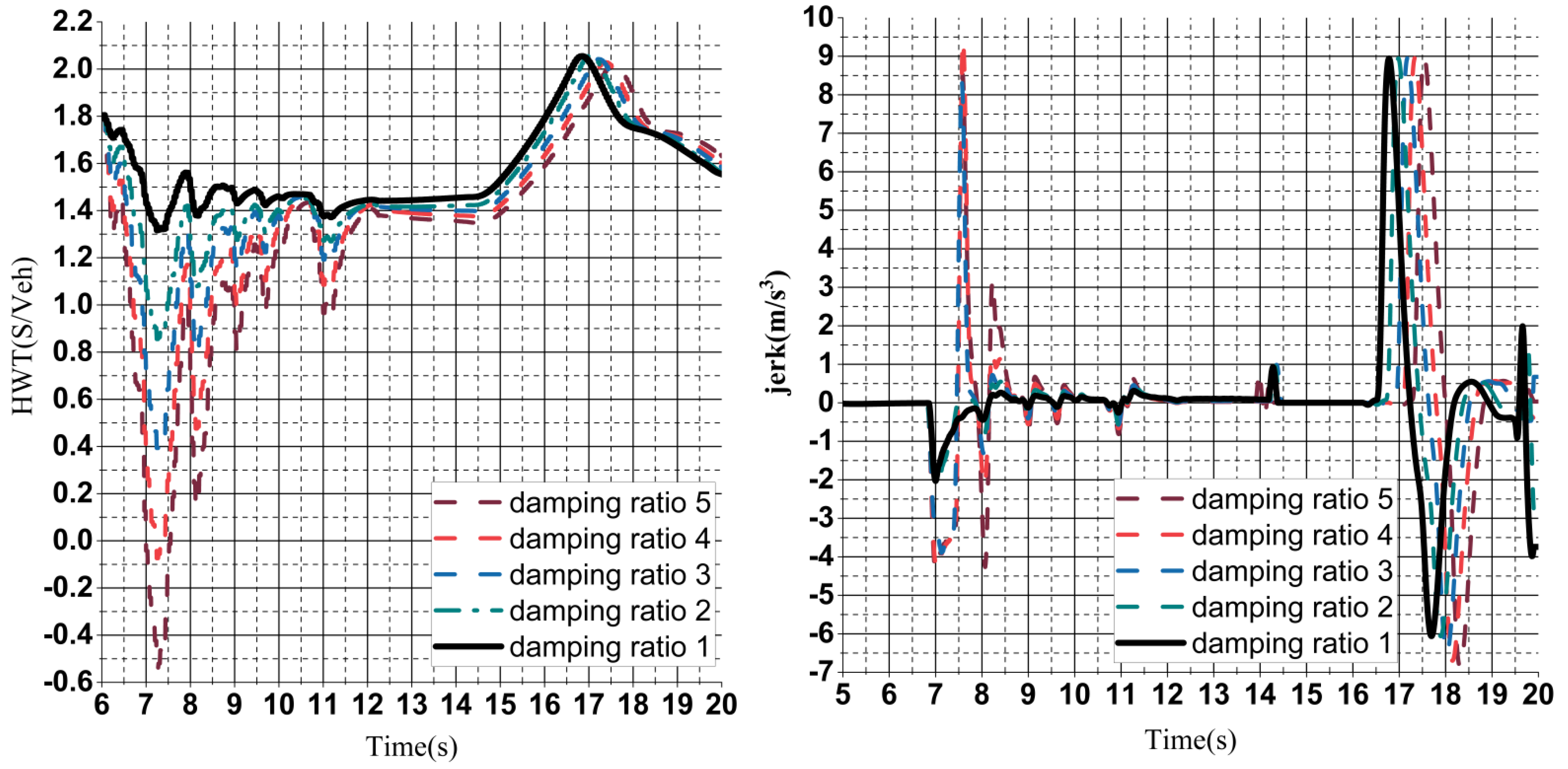
In order to verify the effectiveness of the proposed method, the proposed method is validated by designing a case study for different working conditions and following the vehicle. The validation scheme includes the determination of parameters in the analysis of the flexible decay function, the effect of multi-vehicle following in different operating conditions in the ring simulation, and the effectiveness of stable multi-vehicle following in the actual multi-vehicle following process.

3.2.1. Simulation and Verification of Flexible Fading Algorithm

To verify the rationality and effectiveness of the flexible fading algorithm, in the simulation platform, the cut-in speeds of the cut-in vehicles are set to 10 km/h and 12 km/h, and the queue speed is set to 14 km/h; meanwhile, μ is set to 1–5. The headway time distance of the second vehicle and the jerk are used to evaluate the value range of u. The second following vehicle is used as the evaluation vehicle, whose headway time distance is used to assess its safety, while the jerk is used to assess its comfort, as shown in Figure 6 and Figure 7.

3.2.2. Simulation Verification of Different Working Conditions

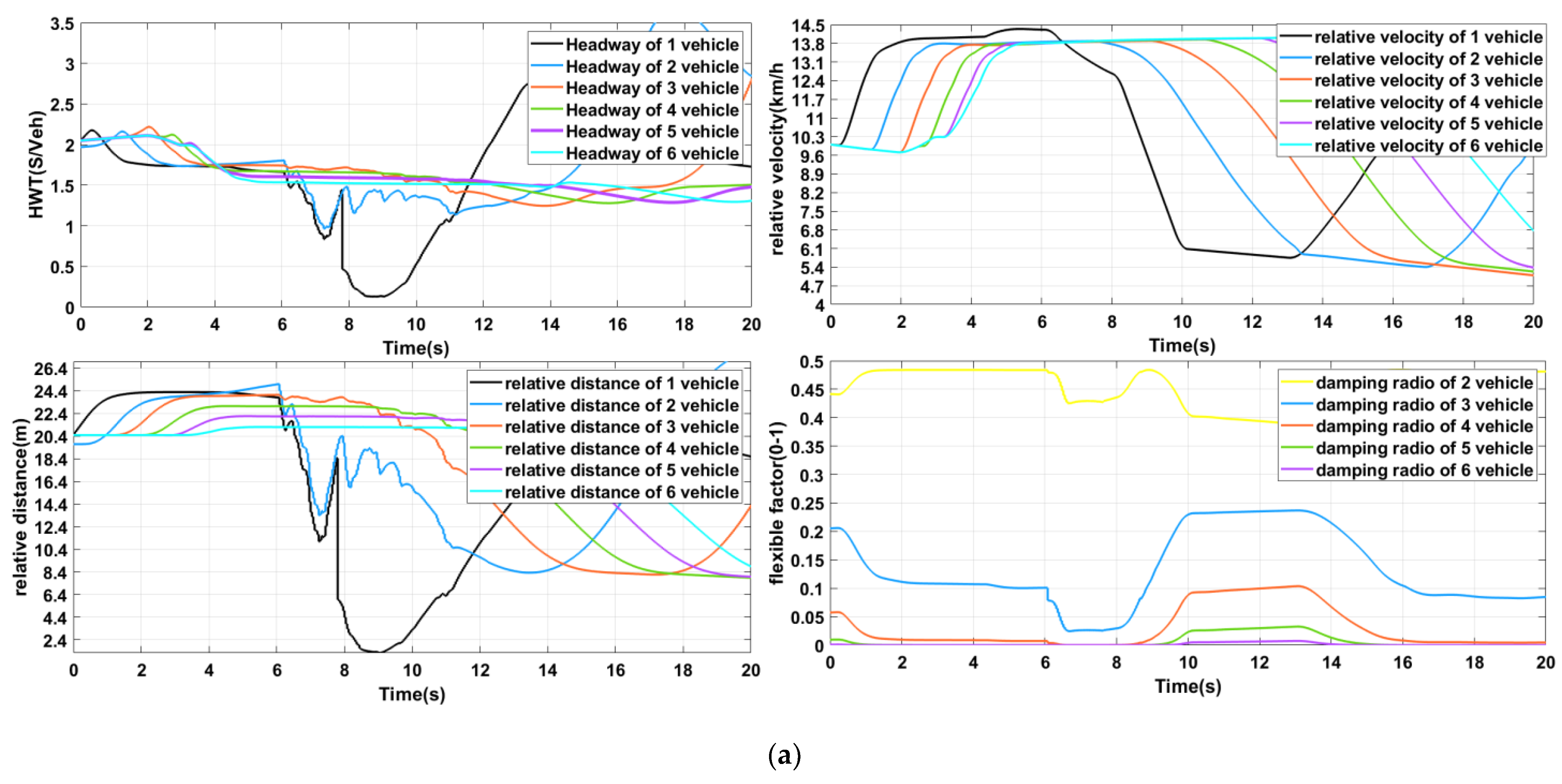
This subsection sets up the CACC algorithm with or without the flexible following factor and flexible attenuation factor optimization under four kinds of bypass lane insertion conditions, and the guiding vehicle in the four cases is set to run at a fixed speed. The initial speed of the rear vehicle is lower than the initial speed of the head vehicle; thus, there is more obvious acceleration following behavior in the initial stage, and this setting also corresponds to the actual real vehicle test. For the above four scenarios, this subsection configures five queue vehicles with CACC control for the overall test. This subsection mainly analyzes and compares the queues of the two types of fleets during the bypass vehicle cutover, and uses the following distance to assess the compactness of the two types of fleets, the headway time distance to assess the following safety, and the jerk to assess the comfort. For notational convenience, the fleet without flexible following factor and flexible decay factor is referred to as CACCNF in this paper (no factor CACC), and fleets with flexible following factor and flexible attenuation factor are CAVF (factor connected and automated vehicle).In the test effect picture, black, blue, coffee, dark green, purple and light green indicate the first car to the sixth car respectively. Also, in the results of the comparison between the two teams, the dashed line indicates the CACCNF team and the solid line indicates the CAVF team.

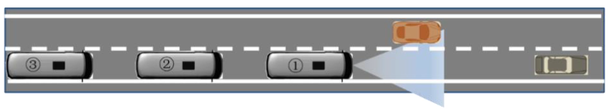
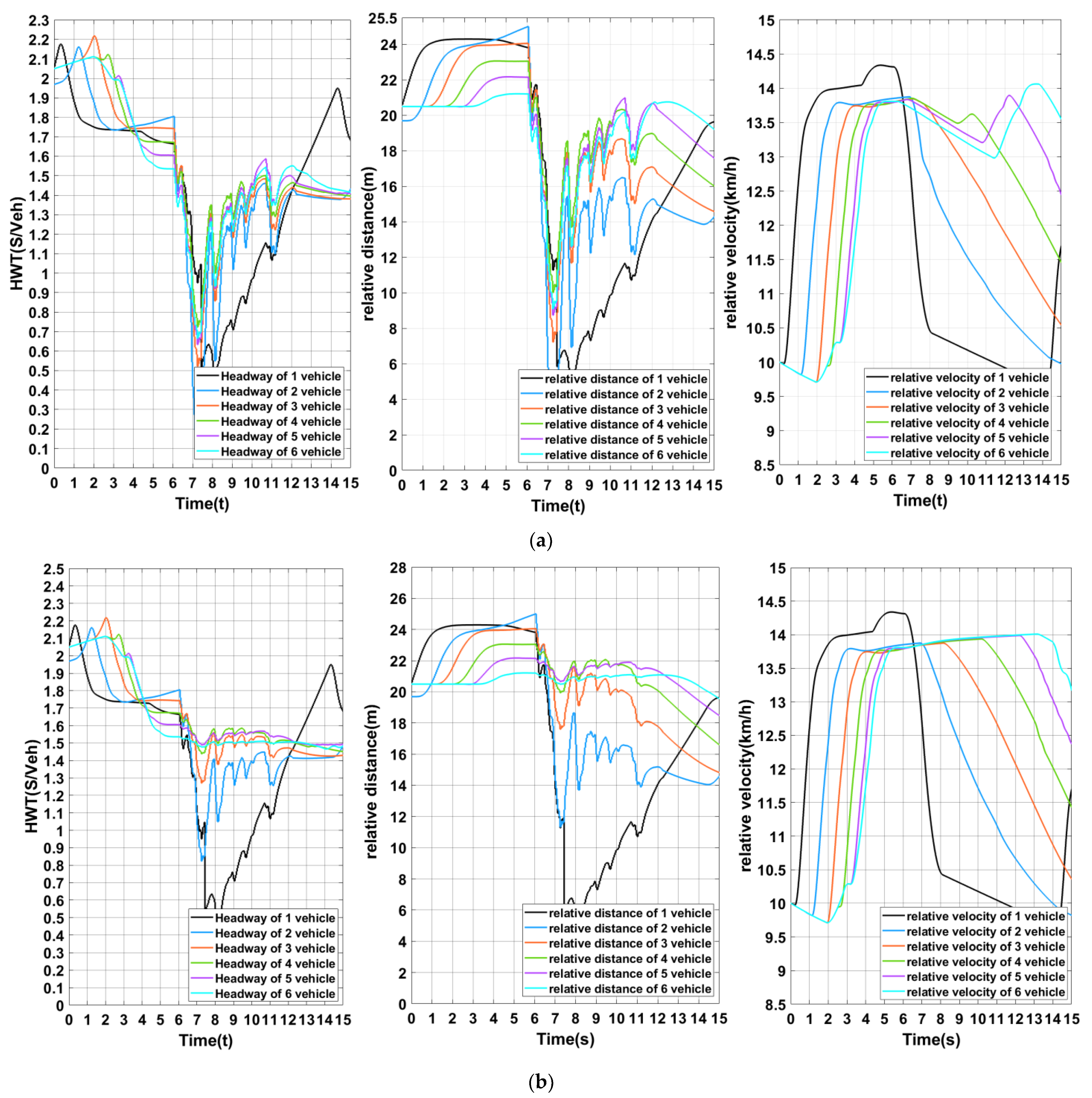
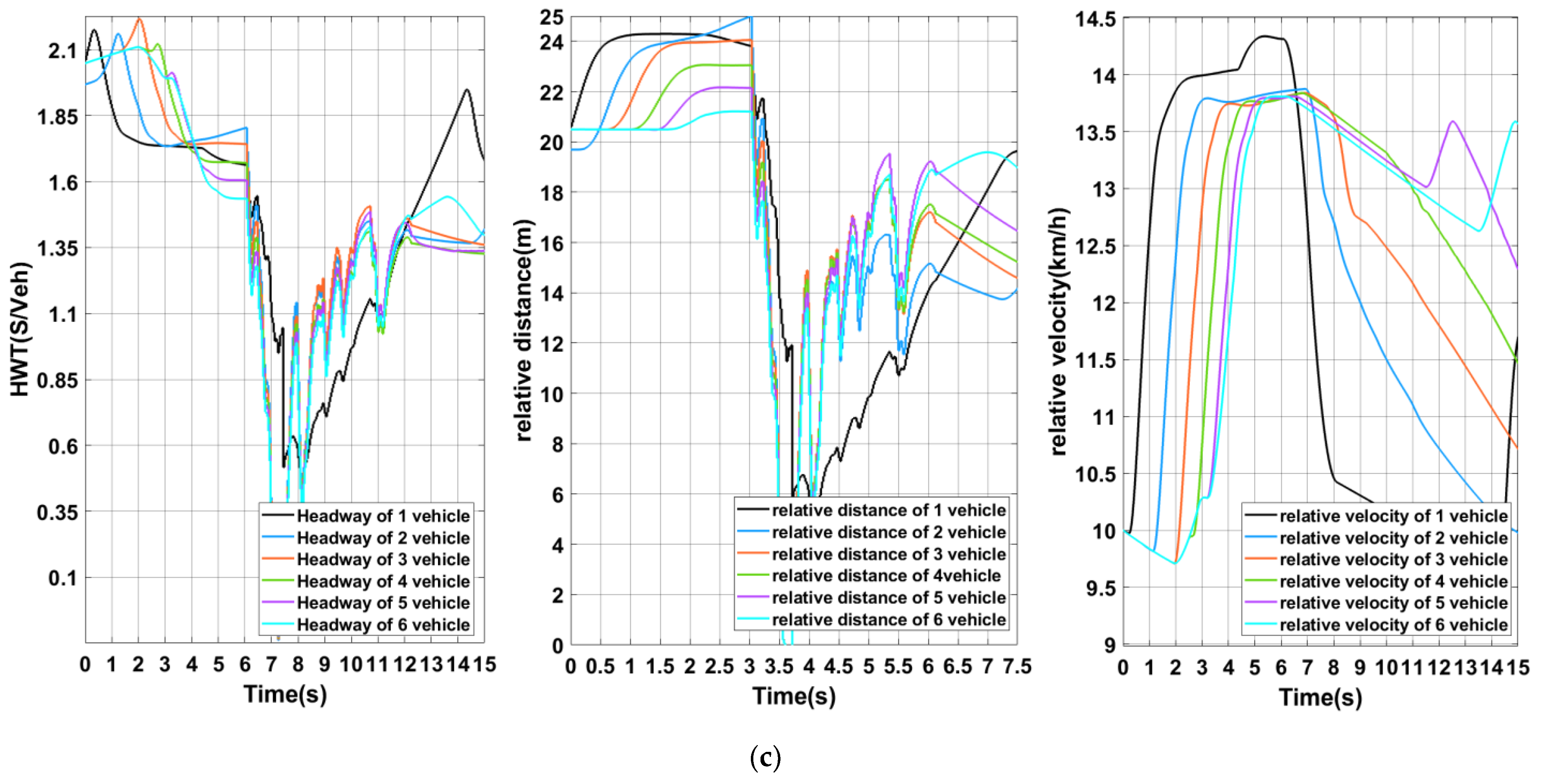
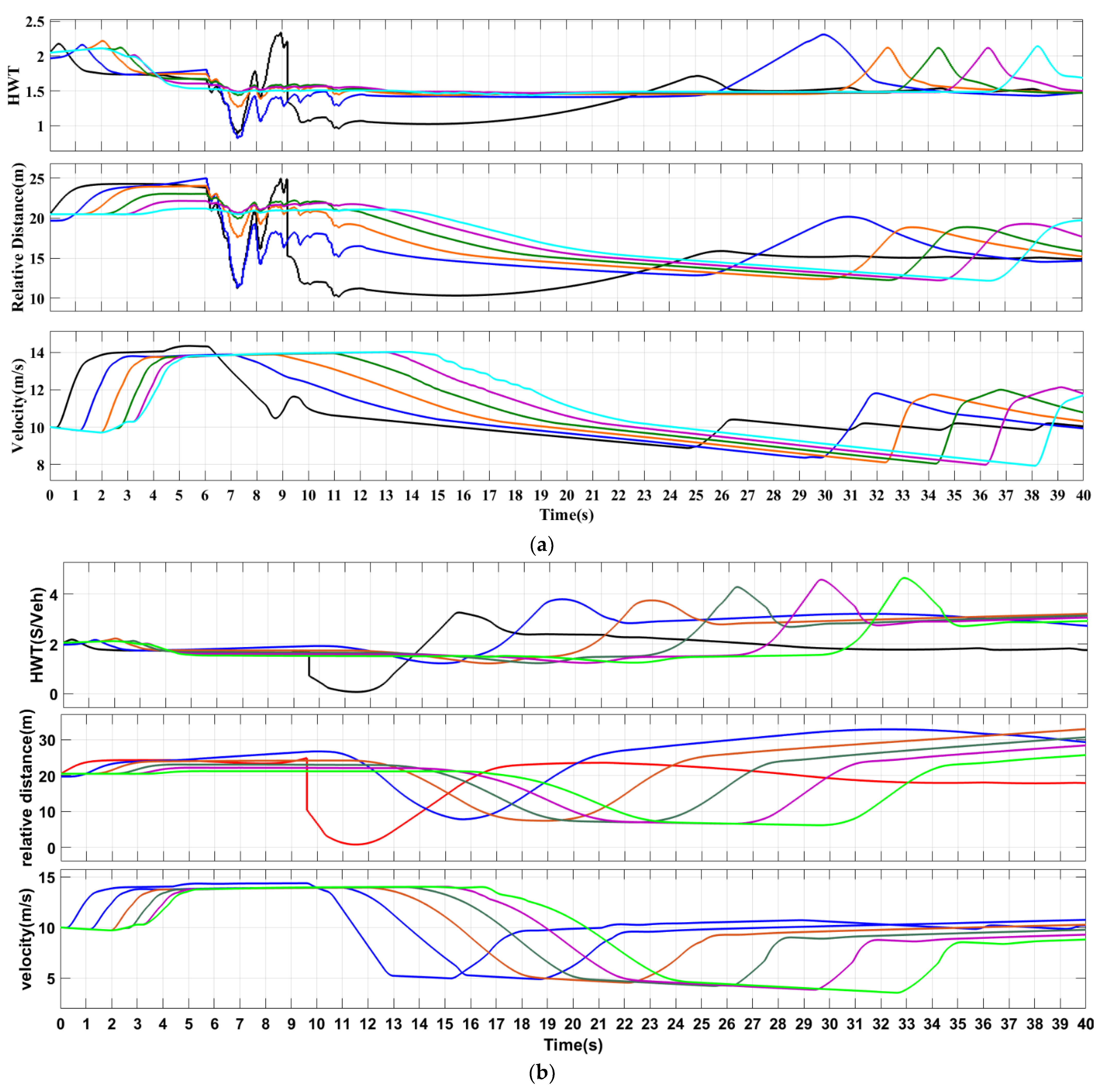
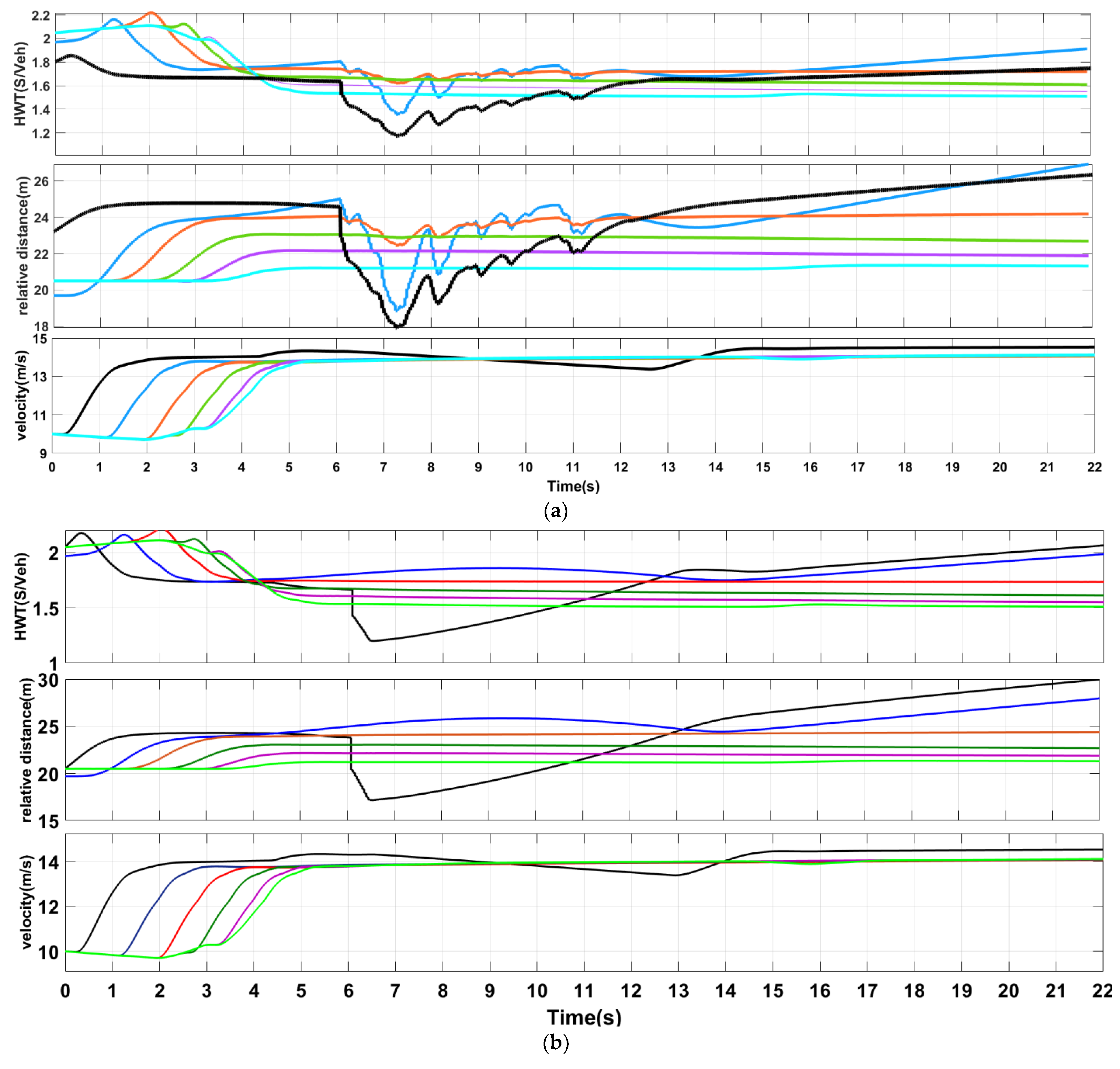
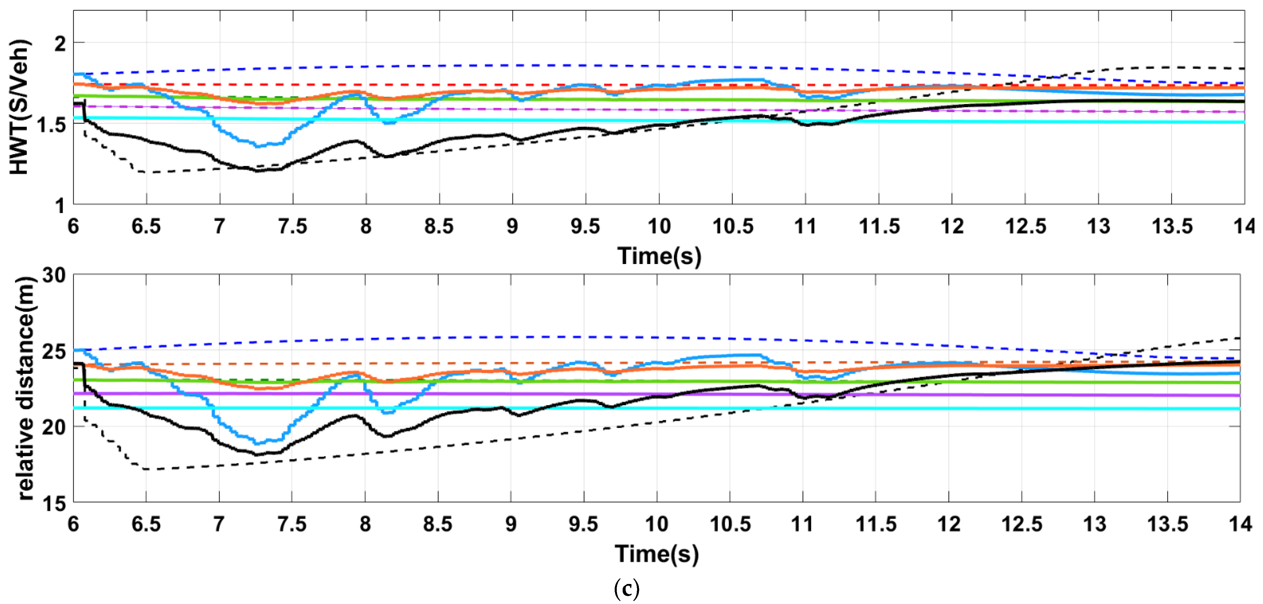
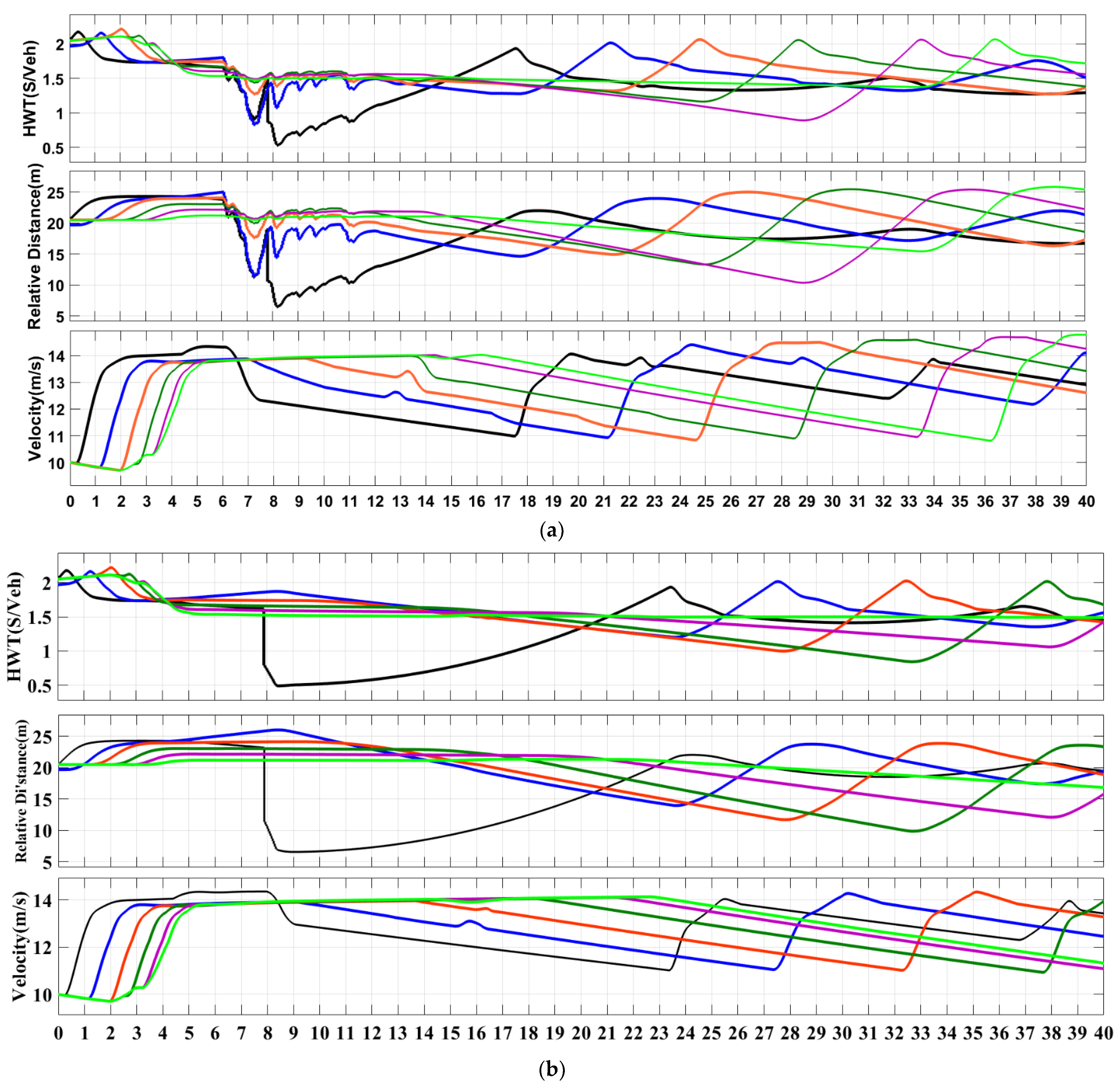
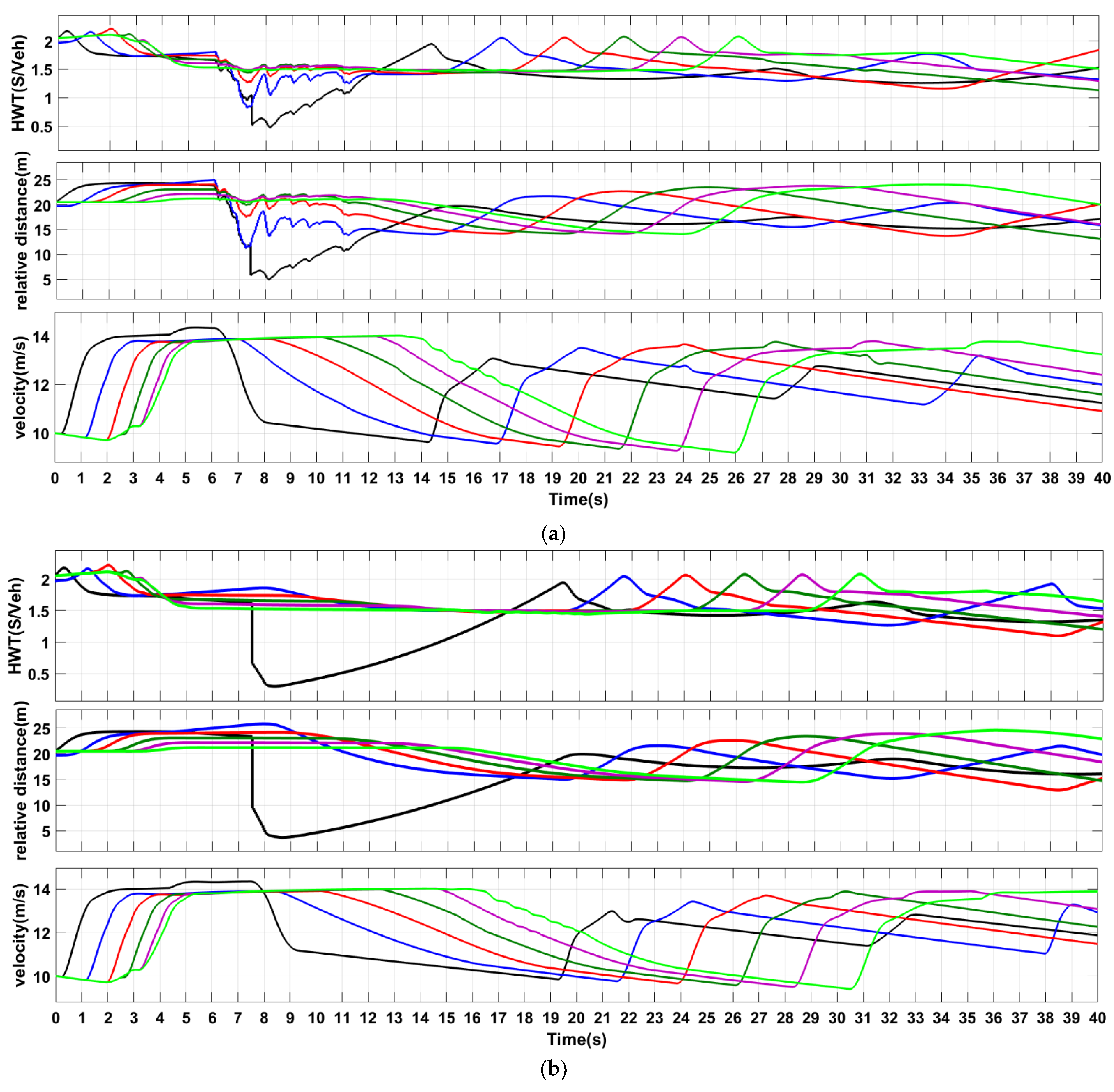
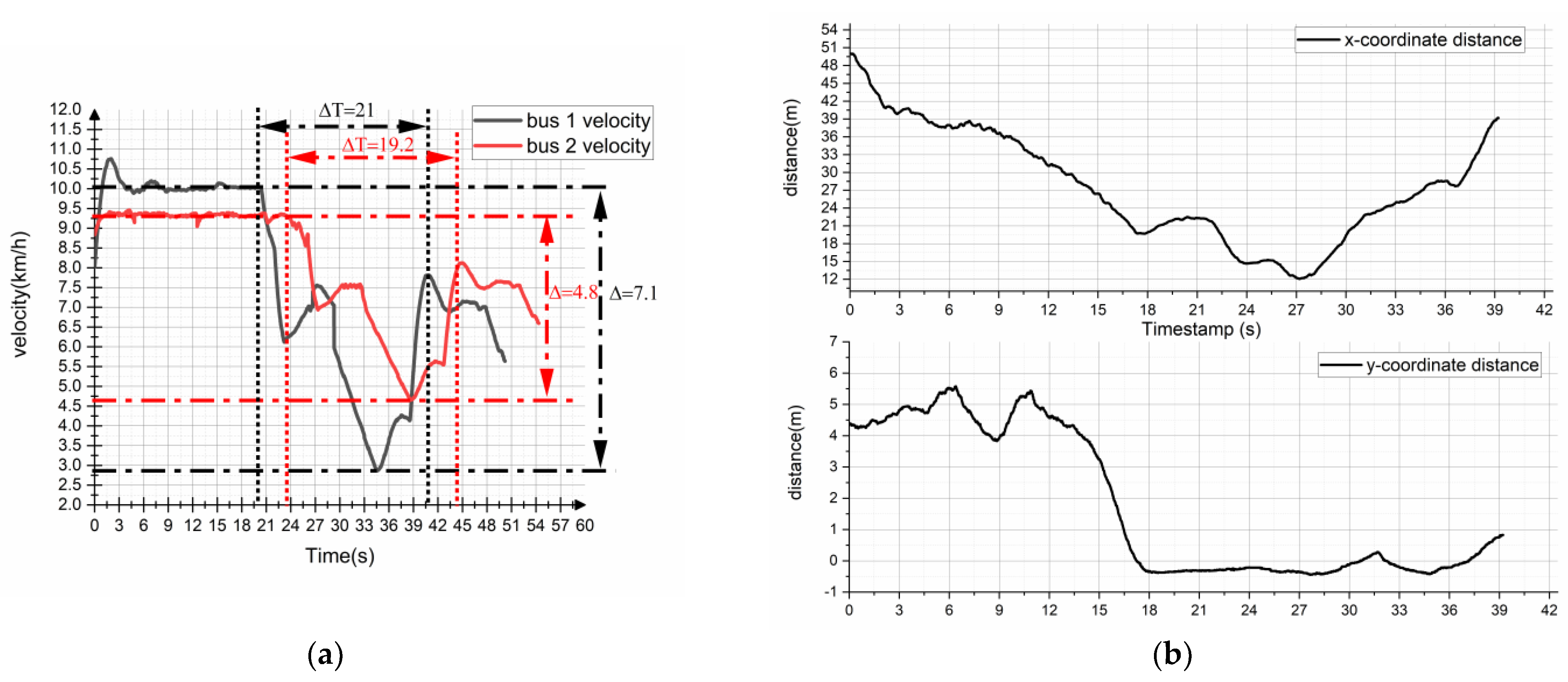
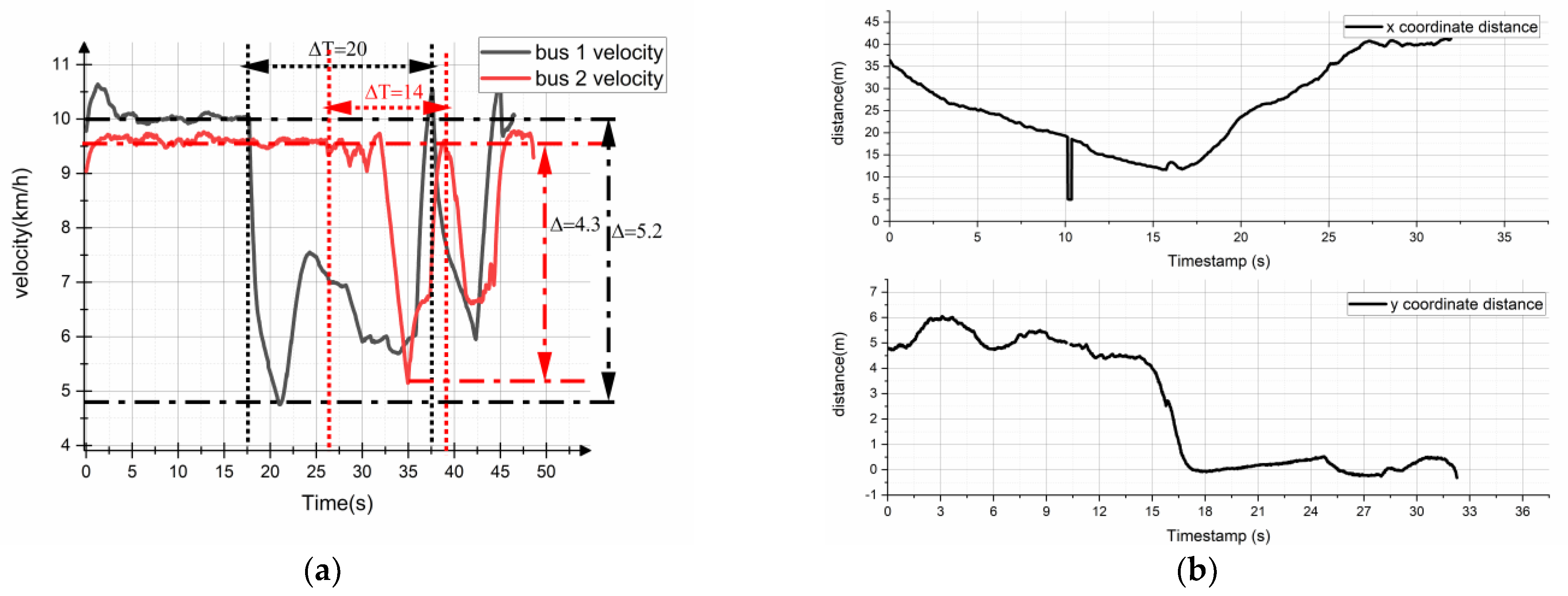
Scenario 1: The vehicle in the side lane cuts into this lane with a constant speed lower than the fleet travel speed of 2 m/s; as the vehicle speed in the side lane is lower than 2 m/s in this lane, i.e., the average speed is 7.2 km/h lower than that of the team train, this speed difference is large, and the limit following the working condition may occur for the train. Therefore, the goal of scenario 1 is to verify whether the algorithm proposed in this paper is safe. The simulation results of the two fleets are shown in Figure 8. Due to the trajectory of the vehicles in the bypass lane being predicted in advance, the CAVF fleet adjusts its speed 3.5 s earlier.

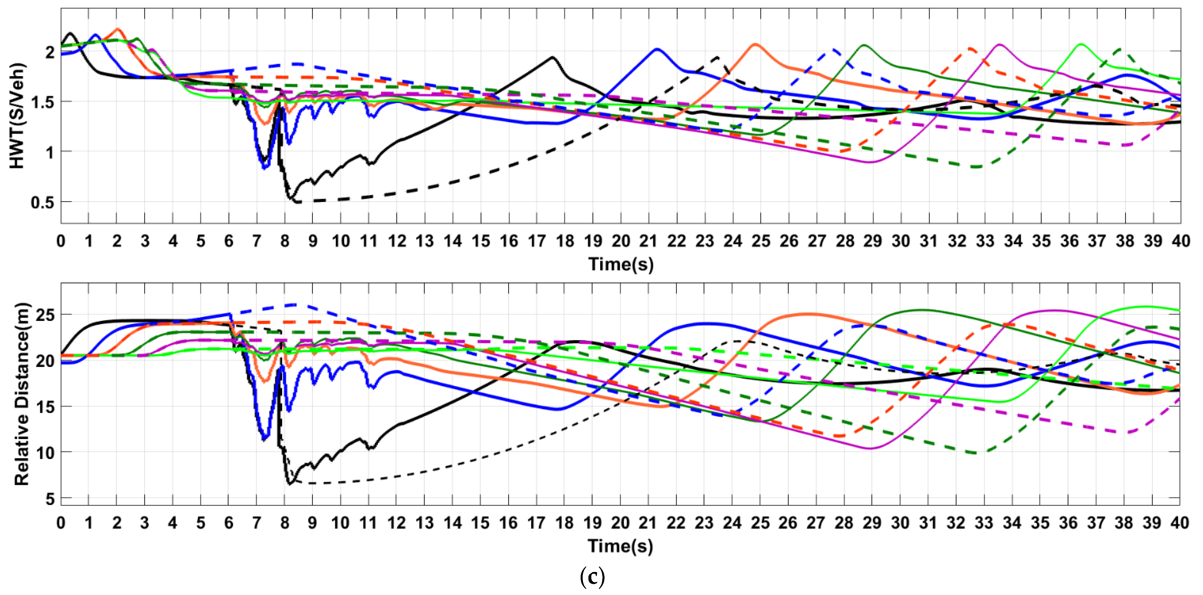
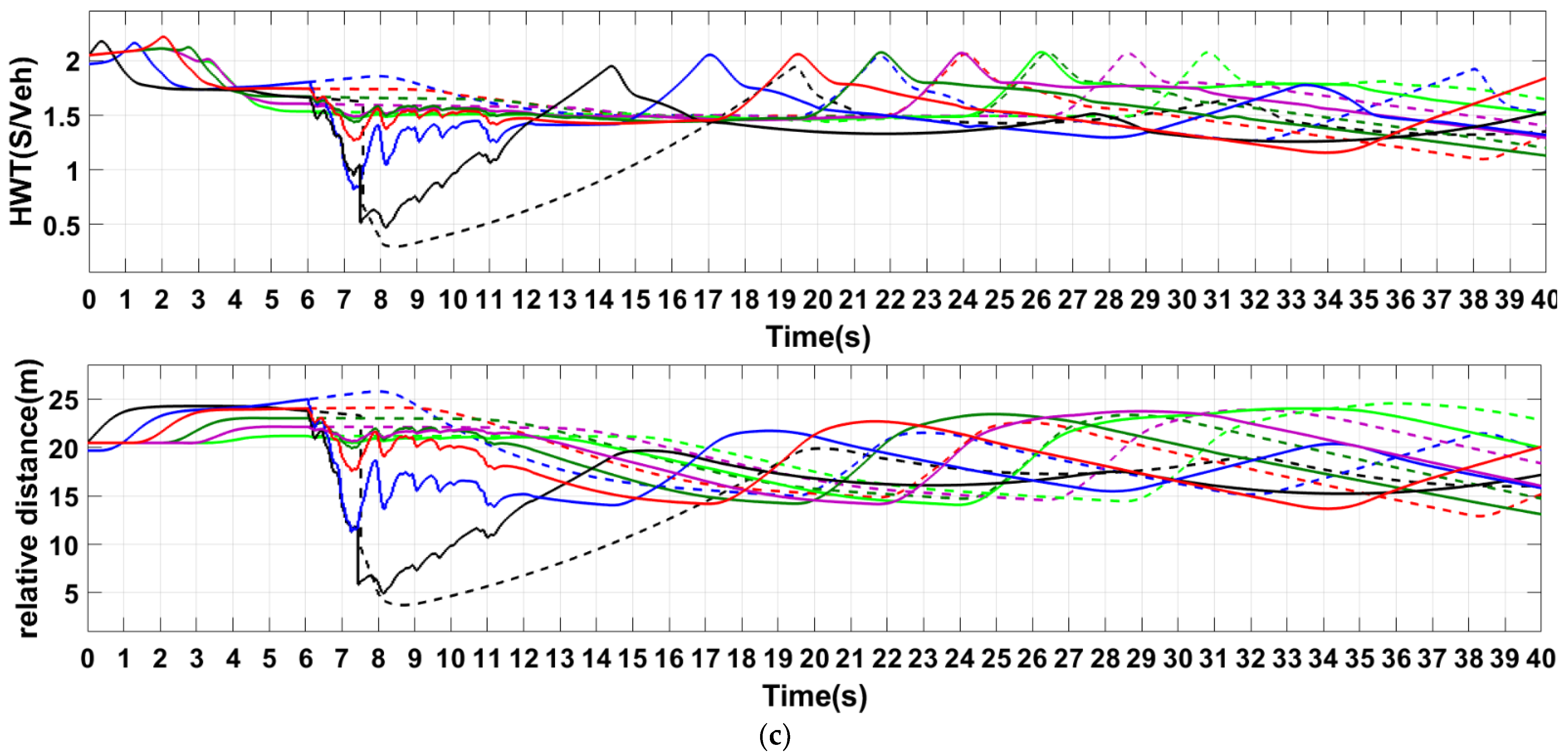
The statistical analysis based on the simulation results of Figure 8 is shown in

Table 1. Follow-up distance and HWT of CAVF and CACCNF teams.

Fleet Number	0	1	2	3	4	5
CAVF-Maximum change in following distance	14.63	13.53	11.59	10.74	9.93	9
CACCNF-Maximum change value of following distance	24.09	25.75	25.63	23.31	21.71	19.42
CAVF-Maximum change in minimum HWT	1.5	1.47	0.94	0.66	0.71	0.64
CACCNF-Maximum change in minimum HWT	3.13	2.5	2.57	2.98	3.34	3.4

. The overall HWT regulation of the convoy is reduced by 65% on average, while the average reduction in the convoy following distance is 49.6%. Therefore, in scenario 1, the CAVF fleet has a smaller and more compact spacing, thereby ensuring safety.

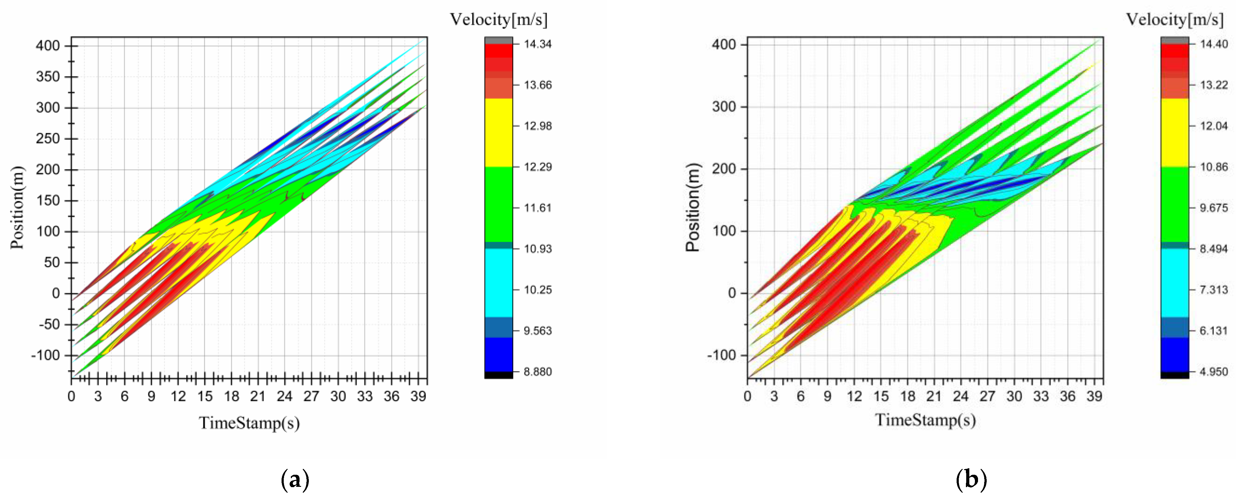
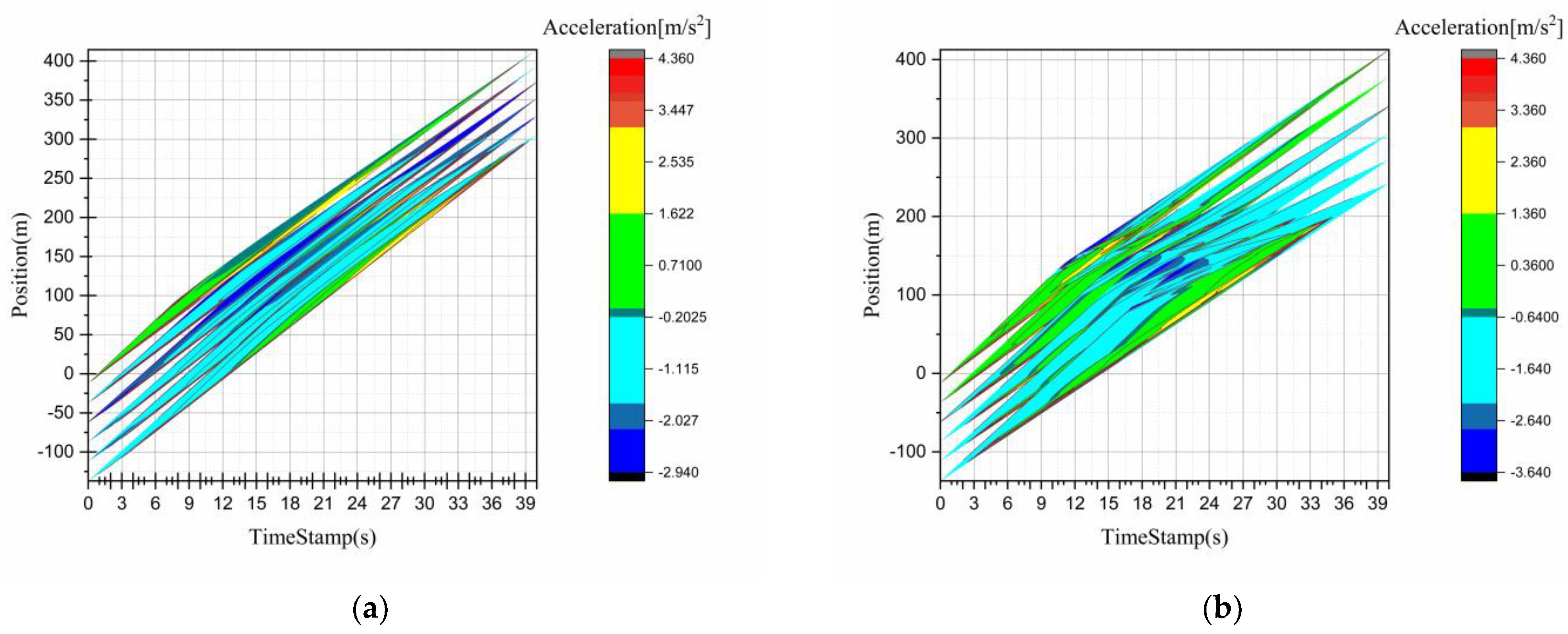
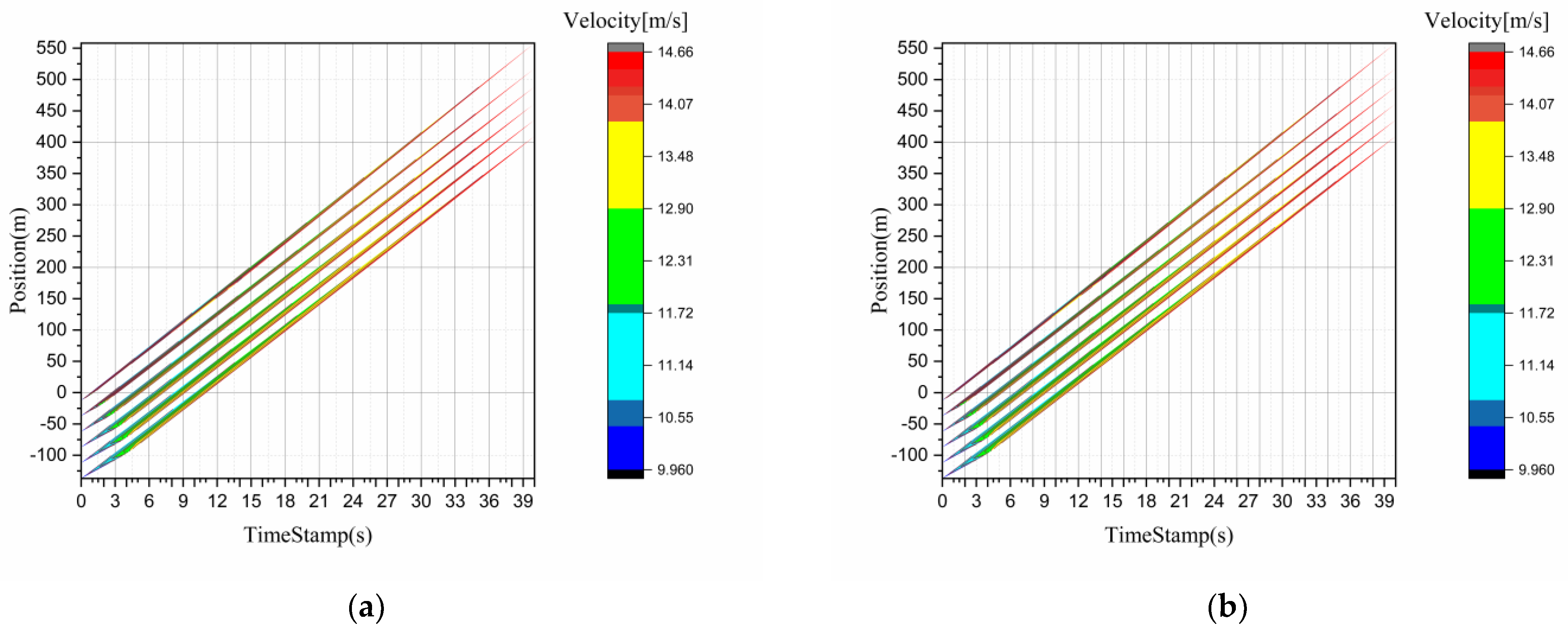
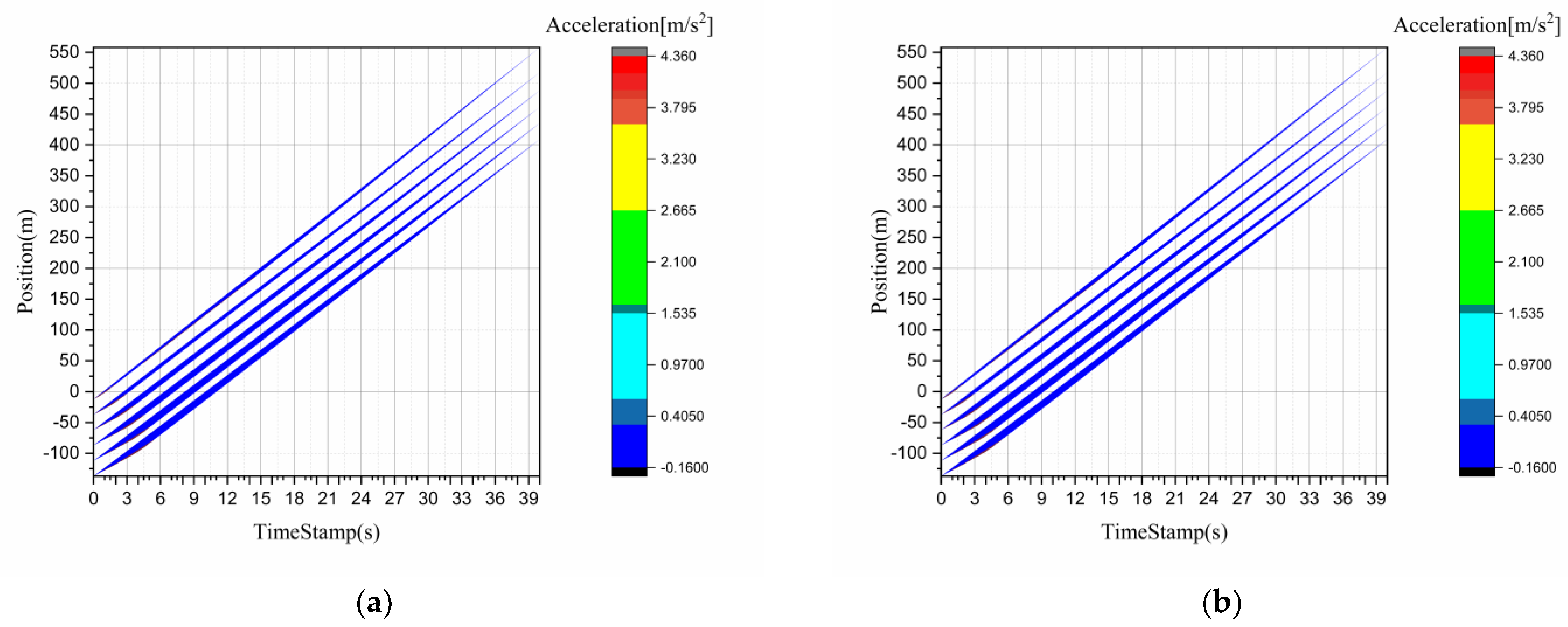
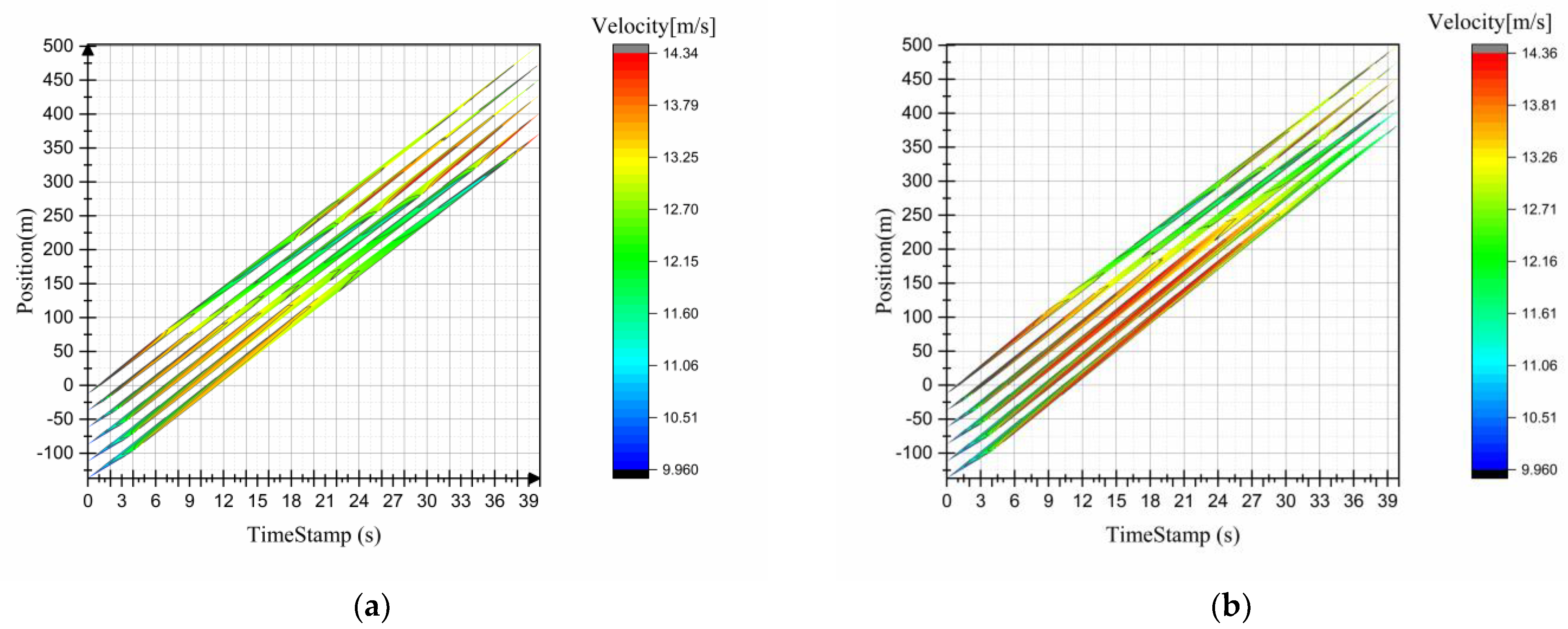
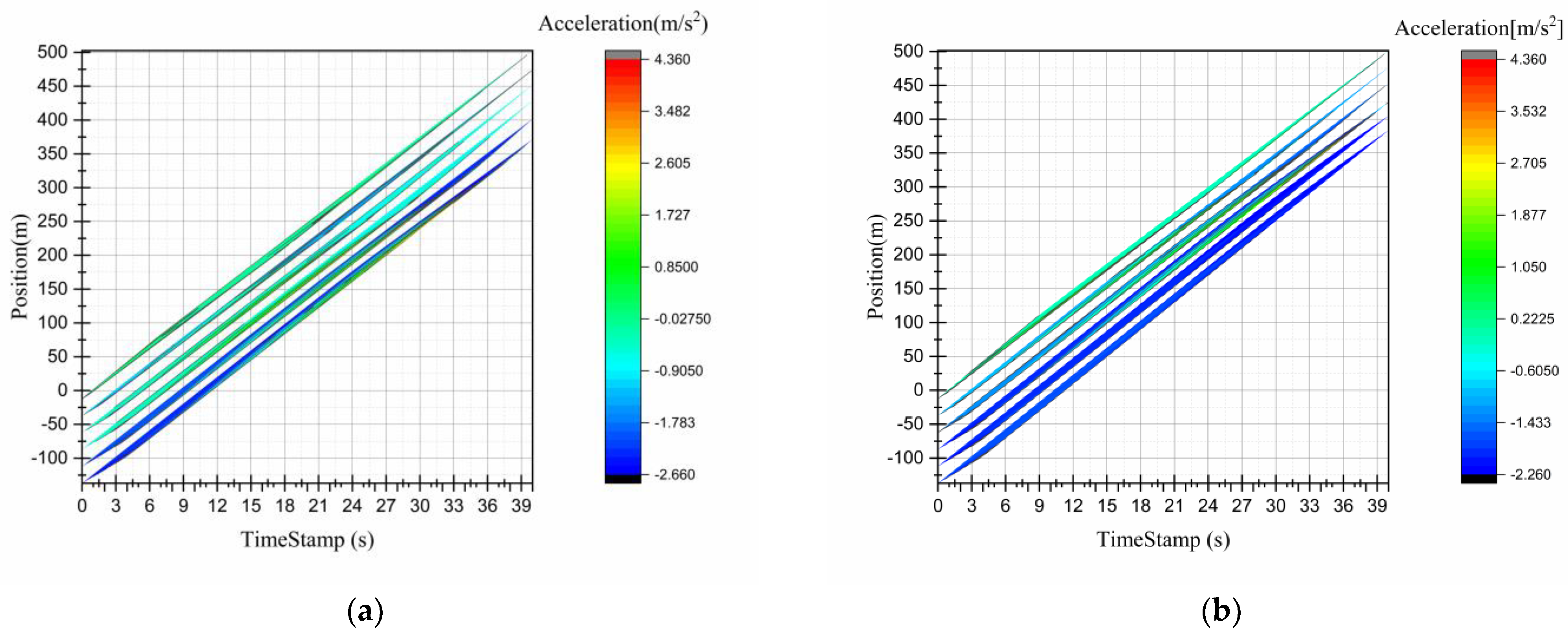
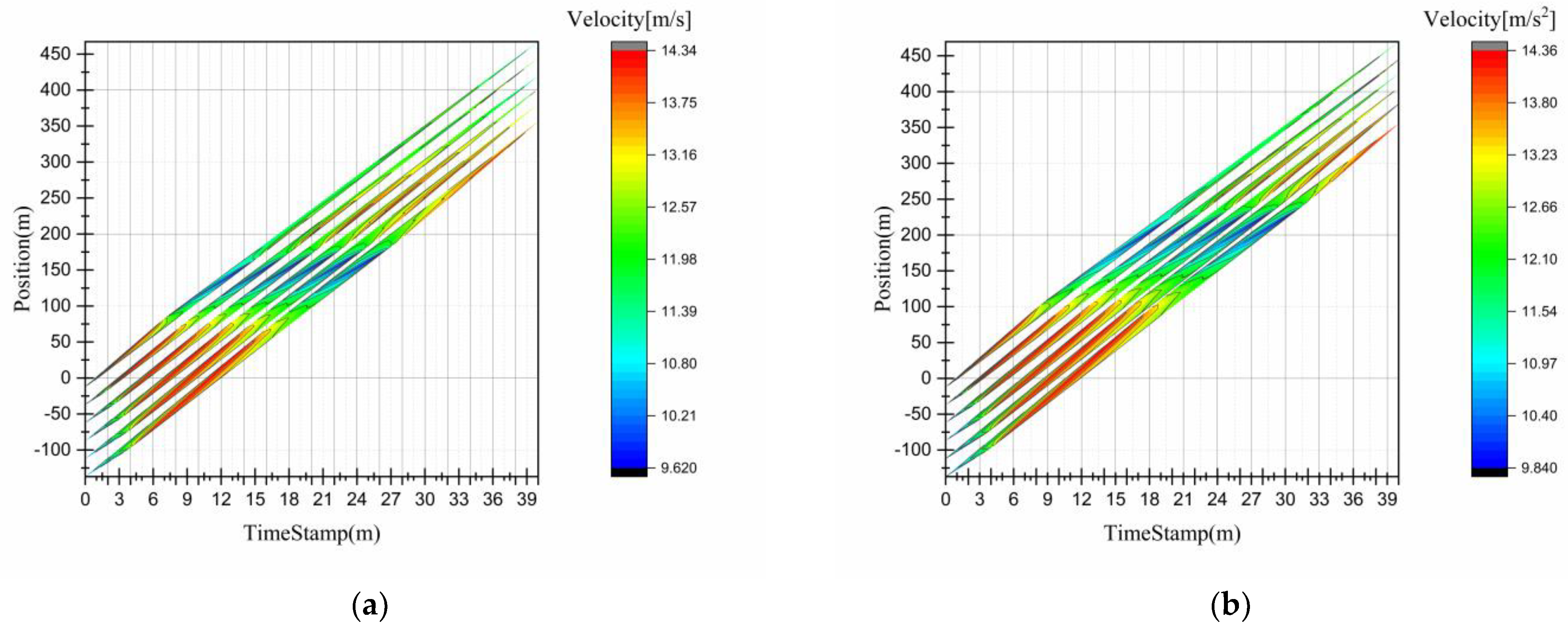
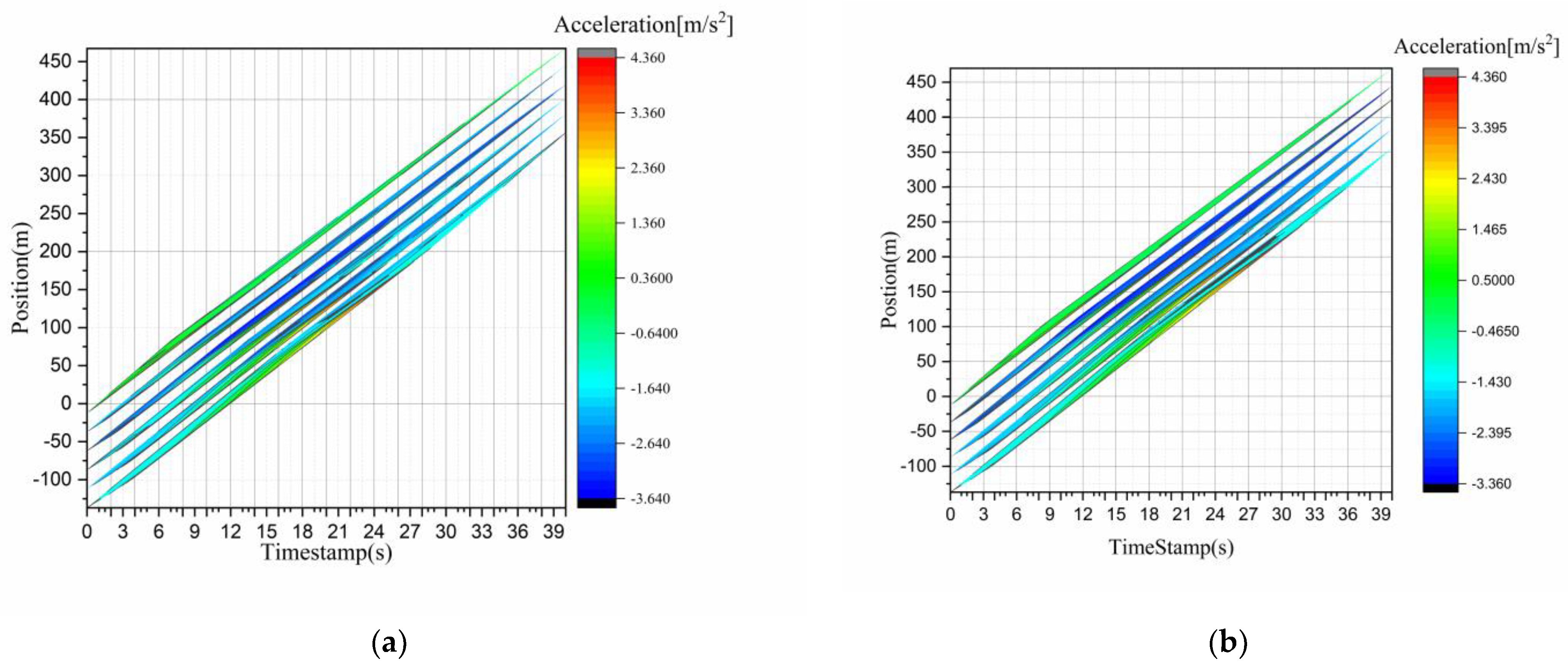
By plotting the velocity and acceleration heatmaps for each vehicle in the CAVF fleet and CACCNF fleet, with time on the horizontal axis and the position of the vehicle on the vertical axis, and by calculating the jerk, the comfort level of the vehicle can be evaluated. As shown in Figure 9.

Based on the results shown in the figure, the following conclusions can be drawn: the acceleration changes in the CACCNF fleet are concentrated from 10 s to 35 s and the acceleration changes are more dispersed, while the acceleration changes of the CAVF fleet are concentrated from 5 to 20 s; after 25 s, the acceleration changes are more concentrated with a smaller change rate and higher comfort. As shown in Figure 10.

The average CACCNF fleet jerk is 54%, and the average CAVF fleet jerk is 48%, representing a 6% increase in comfort. The comfort increase is smaller due to the safety constraints, as shown in

Table 2. Comfort degree of CAVF fleet and CACCNF fleet.

	Queue Serial Number	1	2	3	4	5	6	Average Value
Fleet Type
CACCNF		1.22%	62.9%	62%	64%	66%	69.7%	54%
CAVF		1.65%	7.8%	13%	34%	68%	164%	48%

.

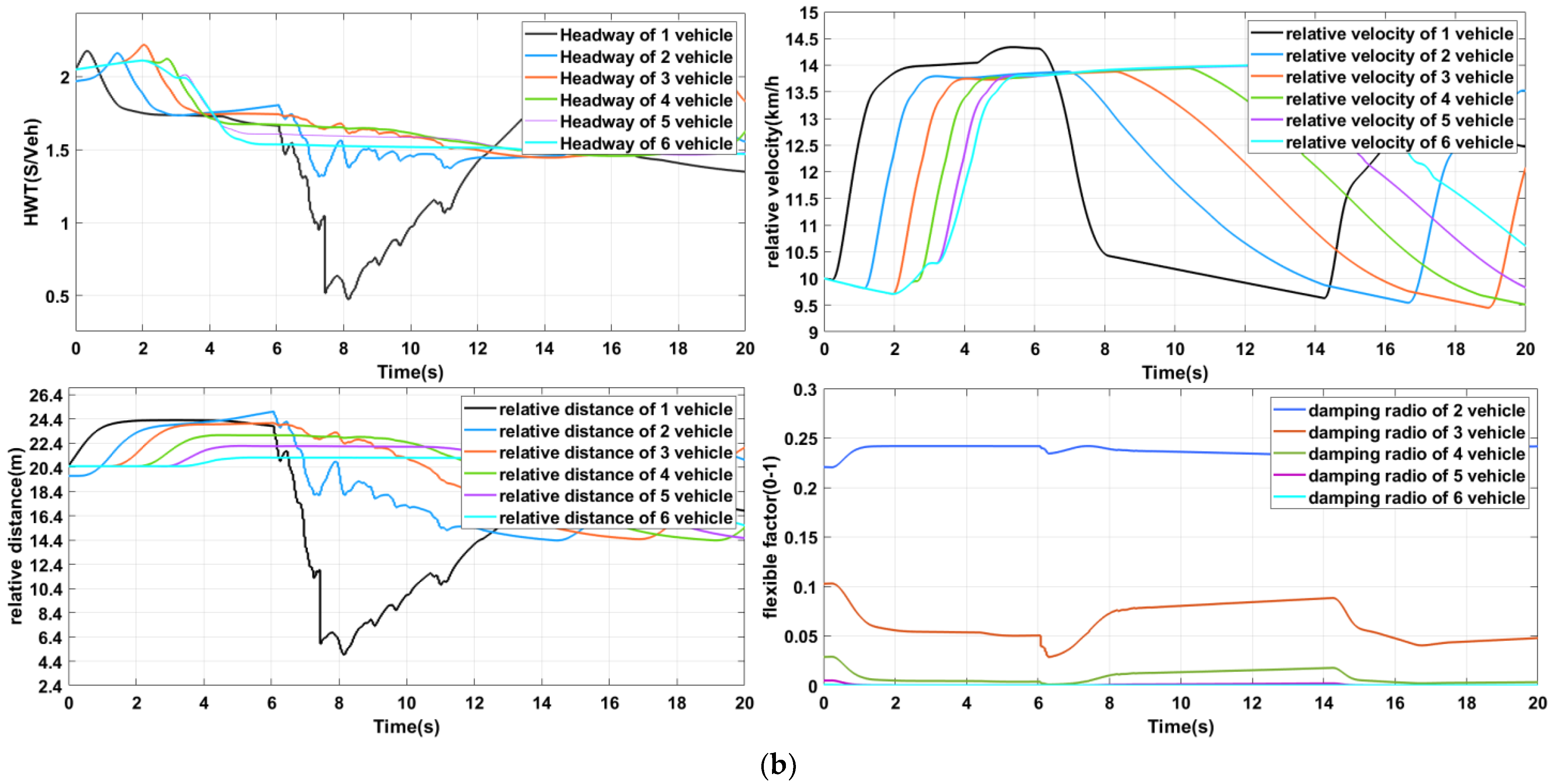
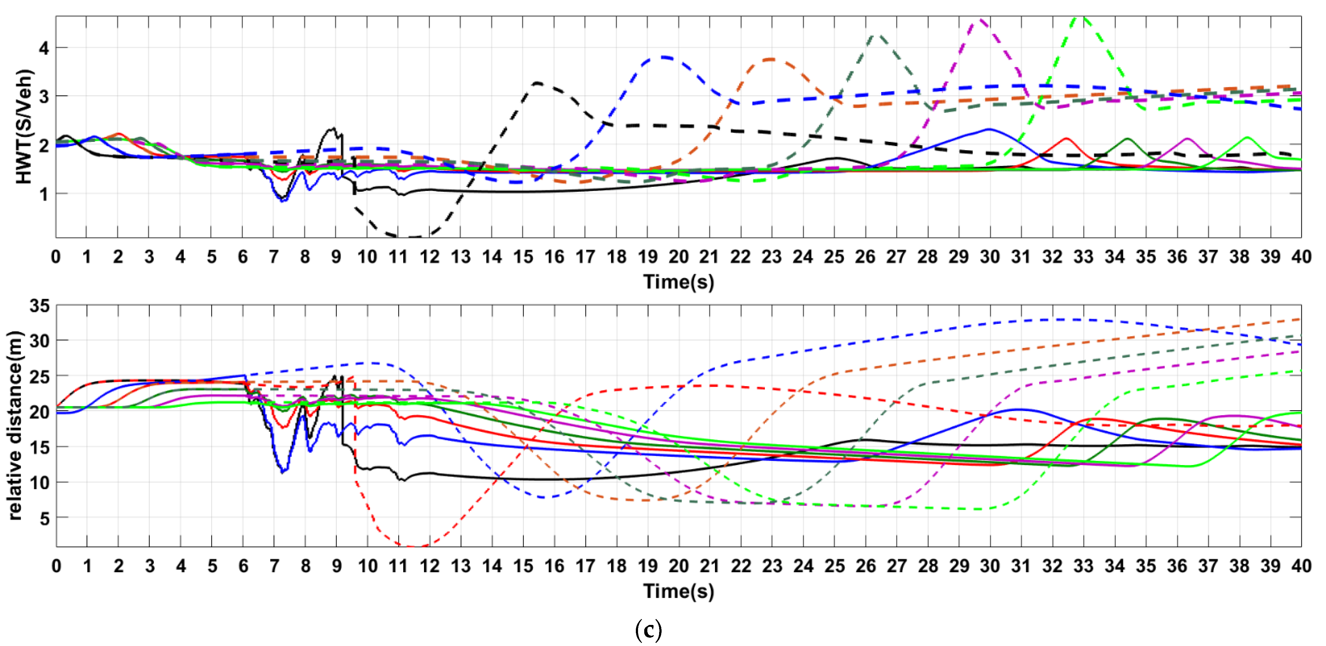
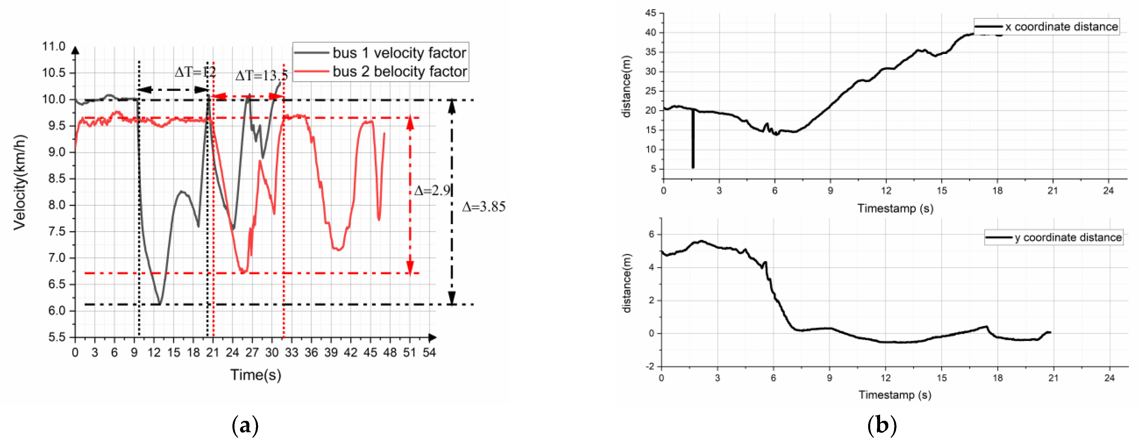
Scenario 2: The side lane vehicles cut into the lane at a higher speed than the fleet travel speed (constant at 2 m/s); because the side car speed insertion is higher than the team train speed (constant at 2 m/s), in the process of cutting in, due to the safety and comfort requirements, the train in the early stage suffers a certain degree of impact, before later converging to the team cruise speed, as shown in Figure 11.

The statistical analysis based on the simulation results of Figure 11 is shown in

Table 3. Comparison table of HWT of CAVF fleet and CACCNF fleet over 20 s.

Queue Serial Number	0	1	2	3	4	5
CAVF Team	1.86	1.78	1.67	1.58	1.54	1.50
CACCNF Team	2	1.92	1.73	1.61	1.55	1.51

. The overall HWT regulation of the convoy is reduced by 65% on average, Meanwhile, according to

Table 4. Comparison of the 20 s follow-up distance between CAVF fleet and CACCNF fleet.

Queue Serial Number	0	1	2	3	4	5
CAVF Team	27.06	25.11	23.49	22.34	21.71	21.23
CACCNF Team	29.05	27.06	24.35	22.74	21.90	21.33

, the average reduction in convoy following distance is 3.3%. Therefore, in scenario 1, the CAVF fleet has a smaller and more compact spacing, thereby ensuring safety.

By plotting the velocity and acceleration heatmaps for each vehicle of the CAVF fleet and CACCNF fleet, with time as the horizontal axis and the position of the vehicle as the vertical axis, and by calculating the jerk, the comfort level of the vehicle can be evaluated. From the results displayed in Figure 12, it can be concluded that the speed of the CAVF fleet and CACCNF fleet varies more in the time domain of 5–15 s for CAVF, but the results also guarantee a tighter fleet in this scenario. As shown in Figure 13, the acceleration distribution of this condition is not obvious; thus, this condition is not compared.

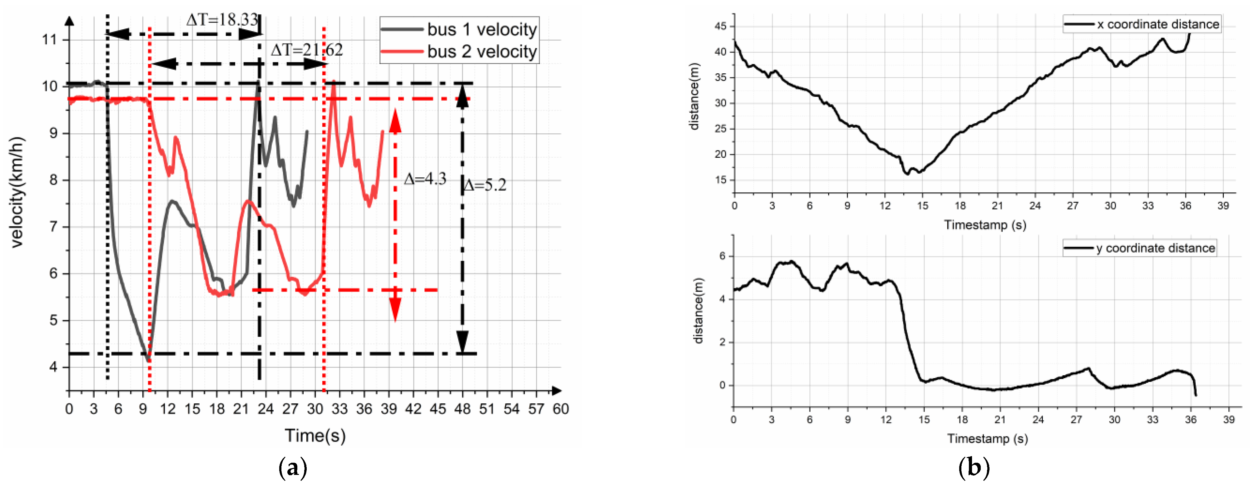
The side lane vehicle cuts into this lane, driving with a positive variable speed and an acceleration higher than the initial speed of the team train. As shown in Figure 14, in the CACCNF fleet, because the side lane vehicle accelerates into this lane and the speed is higher than the speed of the team train, the traffic oscillation changes gradually from the head vehicle to the tail vehicle, and the deceleration process of the head vehicle, as well as the speed change process, is longer, which leads to the back vehicles undergoing real-time speed changes to protect the stability of the vehicle. The time domain of speed change of the CAVF fleet is reduced by 2 s, and the fleet stability is reached more quickly.

The statistical analysis based on the simulation results of Figure 14 is shown in

Table 5. Poor adjustment of follow-up distance and HWT of CAVF and CACCNF teams.

Fleet Number	0	1	2	3	4	5
CAVF-Maximum change in following distance	15.26	8.26	10	11.90	10.95	10.26
CACCNF-Maximum change value of following distance	17.36	9.68	12.11	13.75	11.43	9.6
CAVF-Maximum change of HWT	1.39	1.18	0.78	0.89	1.17	0.69
CACCNF-Maximum change value of HWT	1.438	0.8	1.02	1.17	1	0.98
CAVF-HWT adjustment time	11.5	15.29	18.66	22.7	27.8	33.6
CACCNF-HWT adjustment time	15.53	19.14	26.35	31.84	37.34	42

. The HWT adjustment time of the two types of queues reveals that the adjustment time of the CAVF fleet is shorter compared to that of the CACCNF fleet by about 4 s, and the results of the following distance shown in the above figure indicate that the following distance of the CAVF fleet is lower and the spacing is smaller.

As shown below, the heatmaps of velocity and acceleration for each vehicle of the CAVF fleet and CACCNF fleet are plotted separately, with time as the horizontal axis and the position of the vehicle as the vertical axis. From the results shown in Figure 15 and Figure 16, it can be concluded that the velocity density of the CAVF fleet is concentrated in the range of 5–16 s, and the velocity density of the CACCNF fleet is concentrated in the range of 10–26 s. The velocity oscillation time of the CACCNF fleet is longer and the velocity fluctuation is higher compared with the CAVF fleet. Under this condition, the average fluctuation of both fleets is basically the same.

From the results shown in Figure 17, it can be concluded that the acceleration changes in the CACCNF team are concentrated between 10 and 35 s, whereas the acceleration changes in the CAVF team are concentrated between 5 and 20 s; after 25 s, the acceleration changes become more concentrated and the change rate is smaller. As shown in

Table 6. Comfort degree of CAVF fleet and CACCNF fleet.

Vehicle Sequence	1	2	3	4	5	6	Average Value
CACCNF	1	71.4%	76%	76%	77%	76.5%	62.8%
CAVF	1	71.0%	69.8%	70%	56%	57%	53.9%

, the mean jerk value of the CACCNF team is 62.8%, while that of the CAVF team is 53.9%, representing an 8.9% improvement in comfort level.

Scenario 4: The vehicle in the side lane cuts into the lane with a negative acceleration higher than the initial speed of the team train, as shown in Figure 17.

The statistical analysis based on the simulation results of Figure 17 is shown in

Table 7. Poor adjustment of follow-up distance and HWT of CAVF and CACCNF teams.

	Fleet Number	0	1	2	3	4	5
Compare Standards
CAVF-Maximum change in following distance		14.68	7.3	8.49	9.2	9.66	6.43
CACCNF-Maximum change in following distance		19.62	10.79	9.24	8.25	7.5	6.68
CAVF-HWT Maximum change value		1.467	1.23	1.21	0.77	0.61	0.61
CACCNF-HWT Maximum change value		1.65	0.77	0.96	1.16	1.4	1.67

. The regulation of the overall HWT of the fleet is reduced by 13% on average. The regulation rate of the fleet following distance is reduced by 6% on average. The results according to the figure show that the following distance of the CAVF fleet is lower, and the spacing is smaller.

As shown in the figures below, with time as the horizontal axis and the position of the vehicles as the vertical axis, the heatmaps of the velocity and acceleration of each vehicle of the CAVF fleet and the CACCNF fleet are plotted separately. Figure 18 shows that the high-speed density of the CAVF fleet is concentrated within 0–16 s, and the high-speed density of the CACCNF fleet is concentrated within 0–20 s. The velocity fluctuation time of the CACCNF fleet is higher compared to the CAVF fleet, while the speed fluctuation time of the CAVF fleet is longer and the speed fluctuation rate is higher. From the results shown in Figure 19, it can be concluded that the acceleration changes in the CACCNF fleet are concentrated between 10 and 35 s, and the acceleration changes are more dispersed, while the acceleration changes in the CAVF fleet are concentrated between 5 and 20 s; after 25 s, the acceleration changes are more concentrated.

As shown in

Table 8. Comfort degree of CAVF fleet and CACCNF fleet.

	Queue Train Number	1	2	3	4	5	6	Average Value
Queue Type
CACCNF		1	89%	81%	86%	88%	84%	88%
CAVF		1	70%	68%	70%	73%	66%	74.5%

, the average CACCNF team jerk is 88% and the average CAVF team jerk is 74.5%, representing a 13.5% increase in comfort.

3.2.3. Real Vehicle Verification

The real vehicle test, conducted at the Tianjin University automated driving test site, features the BYD SUV parked in the left lane as the vehicle to be cut-in, and the automated driving fleet in the right lane, with the three vehicles separated by about 50 m behind the vehicle to be inserted, and the head vehicle starting as the signal. The vehicle to be inserted cuts into this lane after the speed of the convoy reaches the set speed of 10 km/h and drives at a uniform speed after cutting in. Figure 20 shows the road environment of the test site and the distribution of the vehicles.

During the actual car test, the test scenario and test environment of the two types of fleets are guaranteed to be the same as best as possible, such as the insertion distance and insertion speed of the vehicles in the side lane. The test results of the actual process are shown below (As shown in Figure 21, Figure 22, Figure 23 and Figure 24, two CACCNF fleet tests and two CAVF fleet tests at 10 km/h).

Table 9. Comparison of evaluation parameters of four tests.

Test	Vehicle Type	Speed-Stabilized Time Domain (s)	Maximum Speed Difference (km/h)	Maximum Difference in Relative Distance (m)	Average Speed (km/h)	Jerk Standard Deviation (1)
test 1	An-kai	21	7.1	39	7.32	3.24352
	Zhong-tong	19.2	4.8	20	7.99	2.74873
Test 2-factor	An-kai	18.33	5.2	25	8.2	2.46581
	Zhong-tong	21.62	4.3	-	9.0	2.63709
test 3	An-kai	20	5.2	24.5	8.26	2.87551
	Zhong-tong	14	4.3	-	8.47	2.75222
test 4-factor	An-kai	12	3.85	25	8.84	2.00784
	Zhong-tong	13.5	2.93	25	8.95	2.60395

shows a comparison of the results.

As shown in the above table, the speed stabilization time domain of test 2 and test 4 is basically lower than the speed stabilization time domain of test 1 and test 3 by 1–2 s. The maximum speed difference between test 2 and test 4 is basically smaller than the maximum speed difference between test 1 and test 3 by 2.1–2.6 km/h. The maximum relative distance, i.e., the distance steadily followed by the queue vehicles, is also improved. The average speed of test 2 and test 4 is higher than the average speed of test 1 and test 3. The comfort level of the head vehicle is improved by 26%, and the comfort level of the rear vehicle is improved by 4.5%.

4. Discussion

The cooperative cruise control method described in this paper was implemented from the perspective of multi-vehicle flexible following. Therefore, the validation of the effectiveness of the flexible following algorithm was first performed on the joint simulation platform of Prescan 2019.3 and MATLAB2019/SIMULINK.

The multi-vehicle cooperative following algorithm was verified under four typical working conditions. The trajectory prediction algorithm could predict the future driving trajectory of the self-driving vehicle under four types of scenarios, as well as predict future driving maneuvers. Then, the prediction algorithm proposed in this paper and the cooperative algorithm of the CAVF fleet were comprehensively validated using the autonomous driving prototype platform. A multi-vehicle following test was conducted at the Tianjin University autonomous driving test site. The test results showed that the test prototype accurately identified the side lane vehicles and more accurately predicted the side lane change intention and lane change trajectory, while outputting the overlap degree of the side lane insertion into this lane. Lastly, the flexible following factor of the head vehicle and the flexible decay factor of the fleet train were output. In the cooperative control of multiple vehicles, the head vehicle speed stabilization time domain of the CAVF fleet was reduced by 1 s and 6 s, while the speed stabilization time domain of team train 2 was reduced by 5 s and 8 s compared with the fleet without the flexible following factor and flexible attenuation factor. The comfort level was improved by 26% and 25%, respectively, the fleet spacing was reduced by 5 m, and the average speed was more tangential to the bypass lane. The CAVF team is more comfortable than the CACCNF team, with a more compact workshop space.

This paper develops a flexible following cooperative control strategy for queues based on vehicle prediction in the side lane. The strategy can control the longitudinal following distance as well as the speed of driverless networked vehicles in the queue by means of a flexible fading factor, flexibly adjusting the following distance, effectively suppressing traffic oscillations in the queue due to the insertion of manually driven vehicles in the side lane, and improving the overall stability of the hybrid fleet and reducing the fleet oscillation rate.

In future work, the approach developed in this paper could be applied not only to advanced driver assistance but also to autonomous driving systems. In the prediction layer, more advanced methods such as asymmetric game theory should be considered so that the prediction layer proposed in this paper can be extended to the remaining complex disclosures, such as intersections.