Article

Modified Whale Optimization Algorithm for Multi-Type Combine Harvesters Scheduling

1
Postdoctoral Station, Henan University of Science and Technology, Luoyang 471000, China
2
Postdoctoral Research Base, Henan Institute of Science and Technology, Xinxiang 453003, China
3
Shenzhen Institute of Advanced Technology, Chinese Academy of Sciences, Shenzhen 518055, China
*
Author to whom correspondence should be addressed.
Machines 2022, 10(1), 64; https://doi.org/10.3390/machines10010064
Submission received: 12 December 2021 / Revised: 8 January 2022 / Accepted: 13 January 2022 / Published: 17 January 2022
(This article belongs to the Topic Motion Planning and Control for Robotics)

Abstract

:
The optimal scheduling of multi-type combine harvesters is a crucial topic in improving the operating efficiency of combine harvesters. Due to the NP-hard property of this problem, developing appropriate optimization approaches is an intractable task. The multi-type combine harvesters scheduling problem considered in this paper deals with the question of how a given set of harvesting tasks should be assigned to each combine harvester, such that the total cost is comprehensively minimized. In this paper, a novel multi-type combine harvesters scheduling problem is first formulated as a constrained optimization problem. Then, a whale optimization algorithm (WOA) including an opposition-based learning search operator, adaptive convergence factor and heuristic mutation, namely, MWOA, is proposed and evaluated based on benchmark functions and comprehensive computational studies. Finally, the proposed intelligent approach is used to solve the multi-type combine harvesters scheduling problem. The experimental results prove the superiority of the MWOA in terms of solution quality and convergence speed both in the benchmark test and for solving the complex multi-type combine harvester scheduling problem.

1. Introduction

As a modern agricultural machine, the combine harvester achieves harvesting at a high speed, playing a significant role in the harvest season [1]. Combine harvesters scheduling, which aims to obtain a reasonable scheduling scheme with the least cost while satisfying various constraints, has attracted research interest across the world. For wheat farms with high yield, harvesters with low capacity may not be suitable. Nik et al. adopted multi-criteria decision-making to optimizing the feed rate in order to match harvesters with farms [2]. In order to improve the harvesting efficiency, Zhang et al. proposed a path-planning optimization scheme based on tabu search and proportion integral differential (PID) control, which effectively shortens the harvesting path [3]. In order to obtain a corner position from the global positioning system, a conventional AB point method is generally adopted, but this is fairly time-consuming. In the light of this, Rahman et al. presented an optimum harvesting area of a convex and concave polygon for the path planning of a robot combine harvester, which reduces crop losses [4]. Due to changes in the location of fruit in the picking process, locating fruits and path planning, which have to be performed on-line, are computationally expensive operations, and hence Willigenburg et al. presented a new method for near-minimum-time collision-free path planning for a fruit-picking robot [5]. Saito et al. developed a robot combine harvester for beans, and this robot can unload harvested grain to an adjacent transport truck during the harvesting operation, improving the harvesting capacity by approximately 10% [6]. The minimization of harvesting distance and the maximization of sugarcane yield, which are conflicting, are treated as optimization objectives. To solve the problem, Sethanan et al. devised a multi-objective particle swarm optimization method, which provides planners with sufficient options for trade-off solutions [7]. Zhang et al. investigated the emergency scheduling and allocation problem of agricultural machinery and propose two corresponding algorithms, based on the shortest distance and max-ability algorithms, respectively [8]. Cao et al. divided the multi-machine cooperative operation problem into two parts: task allocation and task sequence planning. They established the problem model considering both path cost and task execution ability, solving it using an ant colony algorithm [9]. Lu et al. proposed a working environment modeling and coverage path planning method for combine harvesters that precisely marks the boundaries of the farmland to be harvested and effectively realizes the coverage path planning of combine harvesters [10]. Hameed considered that a large proportion of farms have rolling terrains, which has a considerable influence on the design of coverage paths [11].
Furthermore, terrain inclinations are also taken into account by energy consumption models, in order to provide the optimal driving direction for agricultural robots and autonomous machines. Cui et al. mainly investigated the path planning of autonomous agricultural machineries in complex rural roads, employing a particle swarm optimization algorithm to search for the optimal path [12]. In addition, to solve the problem of the slip and roll of autonomous machinery caused by complex roads, a machinery dynamic model considering road curvature and topographic inclination was established to track the planned path. A route planning approach for robots was developed in [13], which was used in orchard operations possessing the inherent structured operational environment that arises from time-independent spatial tree configurations. In conclusion, the studies mentioned above mainly focused on single-type agricultural machinery and seldom involved multi-type agricultural machinery. Combine harvesters scheduling problems, in particular, have not been well studied. However, in view of the household contract responsibility in China, it is essential that multi-type combine harvesters are used for harvesting. The optimization task for combine harvesters is a mixed-integer optimization problem, similar to job-shop scheduling problems [14,15,16], and calls for strong computational tools.
For decades, swarm intelligence heuristic techniques such as particle swarm optimization (PSO) [7,12,17], grey wolf optimization (GWO) [18], ant colony optimization (ACO) [19,20], genetic algorithms (GA) [21], artificial bee colony (ABC) [22,23,24], cuckoo search (CS) [25] and meta-heuristic approaches [26], have been a focus of attention. However, conventional intelligence algorithms may suffer from premature convergence, which significantly affects their solving performance. It is essential to develop an efficient algorithm to address the multi-type combine harvesters scheduling problem. The whale optimization algorithm (WOA) is a meta-heuristic algorithm inspired by whales, proposed by Seyedali et al. in 2016 [27], which mimics the foraging behavior of humpback whales to successfully solve some real-world optimization problems [28,29,30,31,32,33,34]. However, WOA is a swarm-based search algorithm and is easily trapped into local optimal solutions. Considering these shortcomings, some improvement to the WOA is made as follows. Firstly, an adaptive convergence factor is introduced into the WOA, which gives the algorithm strong global exploration ability with a larger step in the early stages of the search and enables it to carry out deep exploitation with a shorter step in the later evolution stages. Secondly, when the algorithm runs into prematurity, a mutation strategy is adopted for individuals where the fitness values have not been improved over a series of 10 iterations, to help them escape from local minima. These improvements help to enhance the convergence speed and the solution quality. The improvements are described in more detail in Section 4.
The major contributions of the paper are listed below:
(1)
A novel multi-type combine harvesters scheduling problem is formulated, generation a complex mixed-integer NP hard optimization problem.
(2)
A new modified whale optimization algorithm, namely MWOA, is proposed. The new variant includes an opposition-based learning search operator, adaptive convergence factor and heuristic mutation. The new method is evaluated based on benchmark functions and comprehensive computational studies.
(3)
The proposed intelligent approach is used to solve the multi-type combine harvesters scheduling problem.
The remainder of this paper is organized as follows. The multi-type harvesters scheduling problem is introduced in Section 2. Section 3 expounds the standard whale optimization algorithm (WOA). In Section 4, the design of the proposed MWOA is discussed in detail. The overall performance of the proposed method is studied, and then it is applied to solve the multi-type harvesters scheduling problem in Section 5. Finally, the conclusions are presented, and further research opportunities are suggested.

2. Multi-Type Combine Harvesters Scheduling Problem

2.1. Problem Description

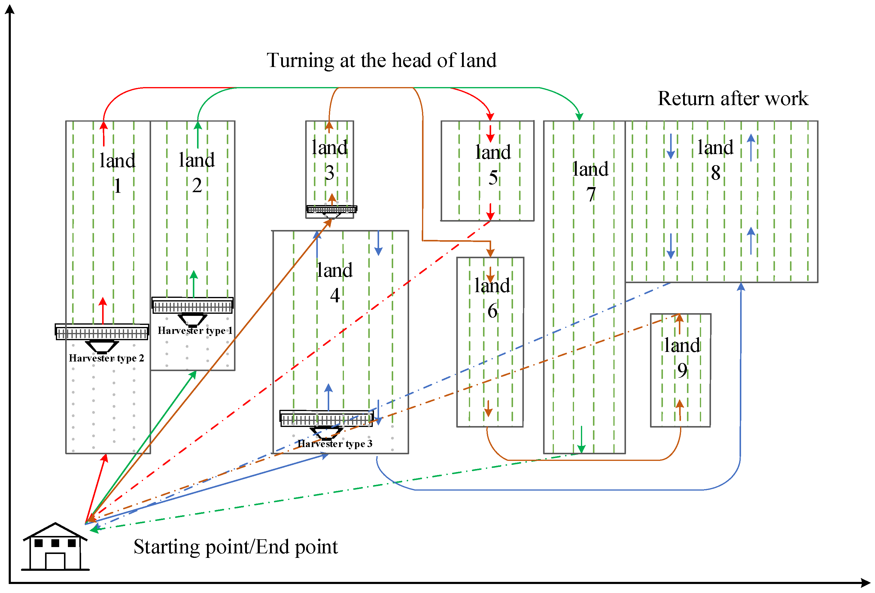
Due to the household contract responsibility system in China and taking into account of the different personnel structure of each family, the amounts of rural land are allocated to each family according to the proportion of family members. The amounts of rural land belonging to each household are therefore different. When the grain in fields is mature and ready for harvesting, multi-type harvesters are in great demand, and it is necessary to make full use of the harvesters. Efficient use also saves fuel and reduces the emission of greenhouse gases. Therefore, it is valuable to investigate how to properly schedule the multi-type combine harvesters to quickly and fully finish the harvesting task. The principle of multi-type combine harvesters scheduling is shown in Figure 1.

2.2. Model Assumptions

The following assumptions are made in this study:
(I)
A single scheduling center is assumed;
(II)
The harvester drives at a constant speed;
(III)
The harvesting demands are known in advance;
(IV)
Harvester faults during harvesting are ignored;
(V)
The time spent on refueling the harvesters is negligible;
(VI)
The time for unloading the harvesters is ignored.

2.3. Notation

The notations used in this paper are summarized as follows.
E : The set of agricultural cooperatives.
G : The set of combine harvesters.
K g : The header width of the combine harvester g , g G .
T g j : The time at which combine harvester g completes harvesting in field j , g G , j D .
R : The set of routes which each harvester travels.
D : The set of the fields ready for harvesting.
S i r : A binary decision variable which indicates whether field i is included in route r or not, i D , r R .
O j r : A binary decision variable which denotes whether combine harvester g covers route r or not, g G , r R .
H i j r : A binary decision variable which indicates whether a combine harvester operates continuous harvesting from field i to field j in route r , i , j D , r R .
D i j : The distance between the harvester and the field, or between the field and the next field, i , j D .
L i , W i : The length and width of field i , respectively, i D .
v g 1 , v g 2 : The driving speed and the harvesting velocity, respectively, of harvester g , g G .
Definition 1.
If the combine harvester is responsible for field i in route r , then S i r = 1 ; otherwise, S i r = 0 .
Definition 2.
If the combine harvester operates continuous harvesting from field i to the field j in route r , then H i j r = 1 ; otherwise, H i j r = 0 .

2.4. Problem Modeling

The aim of this paper is to minimize the time spent on harvesting. The mathematical model, including the objective function and constraint conditions, is defined as follows.
min ( g G r R i D j D ( d i j v g 1 + min { L j v g 2 W j k g , W j v g 2 L j K g } ) H i j r S i r S j r O g r )
s . t .   r R S i r = 1 ,   i D
i D \ { j } H i j r = j D \ { i } H i j r = 1 ,   i , j D ,   r R
K g L i | | W i ,   g G ,   i D
T g 1 i = T g 2 j ,   g 1 , g 2 G ,   i , j D
| G | = | R |
{ r R , e E , j D } H e j r = | R |
{ r R , e E , i D } H i e r = | R |
S i r { 0 , 1 } , i D ,   r R
H i j r { 0 , 1 } , i , j D ,   i j , r R
where objective (1) is to minimize the total time for completing harvesting. Constraint (2) ensures that each filed is visited only once by one combine harvester. Constraint (3) guarantees that a circuit does not exist between field i and field j. Constraint (4) ensures that combine harvester g can enter field i. Constraint (5) indicates that all harvesters complete the harvesting task simultaneously. Constraint (6) means that the combine harvesters continue harvesting. Constraints (7) and (8) require that the start and end points of each route are both agricultural cooperatives. Constraints (9) and (10) are binary decision variables, which only take values of 0 or 1.

3. Traditional Whale Optimization Algorithm (WOA)

To better understand the WOA, it is necessary to elaborate its operating principle. In this algorithm, the positions of humpback whales represent the trial solutions of the optimization problem. If the size of the population and the dimension are Np and d, respectively, the position of the ith humpback whale is expressed as X i = ( x i 1 , x i 2 , , x i d ) , where i { 1 , 2 , N } . The humpback whales utilize a distinctive foraging method called bubble-net feeding to hunt krill or schools of small fishes close to the surface by creating special bubbles along a circle or “9-shaped” path, as shown in Figure 2. The following subsections describe the principle of the WOA exhaustively.

3.1. Encircling Prey

Here, the WOA assumes that the current best solution is the target prey, which provides a referential basis for updating the positions of the other whales. This behavior is expressed in terms of the following equations:
X ( t + 1 ) = X p ( t ) A D
D = | C X p ( t ) X ( t ) |
A = 2 a r a
C = 2 r
a = 2 2 t t max
where t represents the current iteration, X p ( t ) is the position vector of the best solution obtained so far, X ( t ) is the position vector at iteration t , the symbol | · | expresses the absolute value, the symbol is an element-by-element multiplication, r is a random vector in the interval [0,1], a is linearly decreased in the interval [2,0] with an increase in the iteration t and t m a x indicates the maximum number of iterations.

3.2. Spiral Bubble-Net Prey

In this phase, a shrinking encircling mechanism and a spiraling mechanism are adopted to realize normal prey, i.e., humpback whales carrying out shrinking encircling along with spiraling. In this case, the shrinking encircling behavior is still described by Equation (11), while the spiraling behavior can be formulated as follows:
X ( t + 1 ) = D e b l c o s ( 2 π l )   +   X p ( t )
D = | X p ( t ) X ( t ) |  
where D represents the distance between the best solution and the ith whale at iteration t . The parameter b is constant and can be used to control the shape of the logarithmic spiral. The term l [ 1 , 1 ] is a random number.
To emulate spiral bubble-net prey, we suppose that the shrinking encircling and spiraling have equal probabilities, which can be defined as follows:
X ( t + 1 ) = { X p ( t ) A D , p < 0.5 ,     | A | < 1 D e b l c o s ( 2 π l )   +   X p ( t ) ,         p 0.5  
where p [ 0 , 1 ] is a random number.

3.3. Searching for the Prey Following a Whale Selected Randomly

When p < 0.5 and | A | 1 , the current whale will swim toward any whale in the whale population, selected randomly. This operation can be expressed as follows:
X ( t + 1 ) = X r a n d ( t ) A D ,                   p < 0.5 ,     | A | 1
D = | C X r a n d ( t ) X ( t ) |
where X r a n d ( t ) is any position in the whole whale population. In this section, we mainly introduce the basic principles of WOA; the flowchart of WOA is given in Figure 3. The WOA algorithm starts with a random population. At each iteration, whale individuals update their positions according to either a randomly chosen whale or the best whale individuals obtained so far. The parameter α is decreased from 2 to 0, and is used to provide exploration and exploitation, respectively. For updating the positions of the whale individuals, a random whale individual is chosen when | A | 1 , while the best whale individual is selected when | A | < 1 . Depending on the value of p , the WOA is able to switch between either a spiral or an encircling movement. Finally, the WOA algorithm is terminated when the termination criterion is satisfied. Here, the termination criterion is that the maximal evolution generation M a x G e n is reached.

4. Modified Whale Optimization Algorithm (MWOA)

4.1. Opposition-Based Learning Search Operator

The opposition-based learning (OBL) strategy originally proposed by Tizhoosh [35] is a novel technique in computation intelligence and can help to improve the optimization performance of swarm intelligence heuristic algorithms. Specifically, OBL makes effective use of the opposition of the current individuals to gain beneficial information, which may increase the diversity of the population to some extent. With respect to X i j [ L B j , U B j ] , the jth decision variable of the ith individual, the opposite variable can be given by:
X i j = L B j + U B j X i j
where L B j and U B j are the lower and upper boundary of the variable X i j .
In view of the efficiency of OBL, the random search for prey of the WOA can be improved by means of OBL. Therefore, Equations (19) and (20) are substituted by Equation (21):
X i j ( t + 1 ) = L B j + U B j X i j ( t )

4.2. Operator Adaptive Convergence Factor α

By mean of the linear variation of convergence factor α , the WOA simulates the encircling behavior of whales. However, in the course of encircling, fluctuation of the prey population is hard to avoid. That is to say, a linear change of convergence factor seems to affect the whales’ ability to hunt, i.e., the performance of the WOA. To overcome this disadvantage, it is necessary to modify the way that the convergence factor α changes. In view of this, the strategy of a damped oscillation of a sine wave was proposed to guide the change in convergence factor α . This is described in detail as follows. Such a strategy not only ensures that the MWOA rapidly approaches the optimal or a suboptimal solution by a large step in the previous period of the search but also searches around the optimum by a small step in the later evolution stage. Furthermore, on the whole, it implements a decrease in the step despite the oscillation. Meanwhile, the direction of encircling tends to change. Due to these characteristics, the MWOA can achieve a trade-off between exploitation and exploration. The adaptive convergence factor α can be mathematically formulated as follows:
α = 2 e ( 2 tan ( 0.5 π t / t max ) ) sin ( 4.5 π ( 1 t t max ) )
where t is the tth generation.

4.3. Heuristic Mutation

As for the WOA, encircling prey and spiral bubble-net prey approaches both direct the whales to swim forward to particular places where the prey gathers, which likewise makes the whales tend to cluster and lowers the diversity of the population. This results in the loss of the global search ability, and then easily becoming trapped in a local optimal solution. In the following, we introduce improvements to offset this weakness. Generally speaking, the phenomenon of the optimum not being updated for several generations is called a local optimum. With this in mind, we further present a novel heuristics mutation operator, the principle of which is expressed as follows: the whales whose fitness has not improved for 10 generations, and their parents, are selected for mutation. Here, the reason the parents are also chosen is that they may approximate to the optimum, and thus they may help to find the optimum quickly. Through mutation, if a better solution is obtained it is accepted; otherwise, it is discarded. In order to avoid blindness in the mutation strategy, it is reasonable that the mutation probabilities should vary among individuals in terms of their fitness. Furthermore, these individuals, which are trapped in a local optimum, may represent some valuable information; thus, a larger mutation probability p i for an individual i with a smaller fitness not only improves the population diversity effectively but further enhances the global search ability and convergence rate. The mutation probability is defined as:
p i = 1 ( f i t i / f i t max )
where f i t i and f i t m a x are the fitness of the ith whale and the maximum fitness, respectively. To fully excavate the potential information of such individuals, the mutation operator is presented as follows:
X i ( t + 1 ) = N ( X r a n d ( t ) + X i ( t ) 2 , | X r a n d ( t ) X i ( t ) | )
where X i ( t ) and X r a n d ( t ) are the position of the individual i falling into the local optimum and that of the individual generated randomly, respectively. In addition, N ( · ) denotes a Gaussian distribution where the mean and standard deviation are ( X i ( t ) + X r a n d ( t ) ) / 2 and | X i ( t ) X r a n d ( t ) | , respectively.
The pseudocode of the MWOA is shown in Algorithm 1.
Algorithm 1. The pseudocode of MWOA.
1. Initializing a population of N whales with random positions
2. Initializing of parameters
3. Evaluate each whale with the fitness function
4. Record the position of the best whale Xp and the corresponding objective value f(Xp)
5. while the terminating criterion is not satisfied do
6.         for i = 1:N
7.      Update a with Equation (23), A with Equation (13), C with Equation (14), l [ 1 , 1 ] , and p [ 0 , 1 ]   14
8.           if (p < 0.5)
9.                if (|A| < 1)
10.                    Update the position of the current whale according to Equation (11)
11.              else if (|A| ≥ 1)
12.              Update the position of the current whale according to Equation (22)
13.                 end if
14.           else if (p ≥ 0.5)
15.              Update the position of the current whale according to Equation (16)
16.            end if
17.          end for
18. Evaluate each whale with the fitness function
19. Update Xp and f(Xp), if there is a better solution
20. Carry out heuristic mutation where mutation probability is computed with Equation (22)
21. end while
22. return the optimal solution Xp and the corresponding objective value f(Xp)

5. Experiments and Discussion

5.1. Benchmark Functions Test

In this subsection, to analyze and compare the accuracy and stability of the MWOA, the MWOA is applied to solve eight classical benchmark functions with dimensions D = 30, 50 and 100, as listed in Table 1. These functions have the following characteristics: unimodal, multimodal, separable and non-separable, marked as U, M, S and N, respectively, in Table 1. As they have only one local optimum, unimodal functions are easily solved, and the local optimum is also the global optimum. Therefore, the exploitation capability of optimization algorithms is often tested on these types of functions. In contrast, multimodal functions generally have more than one local optimum, and the number of local optima increases with the dimension of the problem, which makes it difficult to obtain optimal solutions. Thus, the exploration ability of optimization algorithms is always tested on multimodal functions. Separable functions are those where a decision variable can be written as the sum of n functions with a corresponding decision variable, and non-separable functions are those where this is not the case. High-dimensional functions expand the solution space exponentially compared to low-dimensional functions, so the high-dimensional case is harder to solve. Considering the above analysis, the selected benchmark functions can effectively evaluate the performance of optimization algorithms in terms of escaping from local optima and convergence speed. The results obtained by the MWOA were compared with nine other optimization algorithms: the original whale optimization algorithm (WOA) [27] and variants of other optimization approaches including HCLPSO [36], ETLBO [37], iqABC [38], SBAIS [39], ECSA [40], ADFA [41], GWO-E [42] and MHS [43].
All experiments in this study were conducted using a PC with a Windows 10 system, 3.4 GHz Intel Core, 16 GB RAM and MATLAB R2014b. For a fair comparison, the number of function evaluations (FES) was utilized to evaluate the performance of the algorithm, i.e., all algorithms in the experiments had the same FES, for example, FES = 80,000 for 30 dimensions, FES = 100,000 for 50 dimensions and the FES = 300,000 for 100 dimensions. The other parameters of the comparison algorithms were the same as those of the corresponding references. For the MWOA, the parameter b was set to 1. Each algorithm had 30 independent runs for each trial.

5.2. Performance Evaluation Compared with Other Algorithms

To test the solution ability of the MWOA, it was compared with the other algorithms using 30-, 60- and 100-dimensional function optimizations. The corresponding results in terms of the minimum “Min”, the mean “Mean” and the standard deviation “Std” of the best-so-far solution, are given in Table 2, Table 3 and Table 4, respectively, where the best results are highlighted in boldface. The Wilcoxon signed-rank test was adopted with a 0.05 significance level to identify the significant differences between algorithms, and the statistical results “Sig” are marked as “+/=/−”, corresponding to cases where the MWOA is better than, equal to or worse than the given algorithm, respectively. Additionally, the mean convergence characteristics of the algorithms are shown in Figure 4 for different dimensional benchmark functions.
From Table 2, Table 3 and Table 4, it can be seen that the performance of the proposed MWOA is equal to that of the conventional WOA for benchmark functions f1 and f6. However, for the rest of the functions, regardless of dimension, the solution quality obtained by the MWOA exceeds all the other algorithms in terms of mean results and standard deviation. Compared with the standard WOA, it can be seen that the MWOA is significantly better. Furthermore, based on the Wilcoxon signed-rank test results, the proposed MWOA demonstrates similar performance. These results all reveal that the MWOA is robust against the dimensionality of the problem to be solved. Furthermore, the results of the MWOA for unimodal functions are better than those for multimodal functions irrespective of dimension, which indicates that the MWOA has strong local search capability. Figure 4 shows the mean convergence characteristics of different functions of various dimensions, reflecting the exploration and exploitation performance of each of the algorithms. It is clear that the performances of different algorithms are very different for different benchmark functions. The convergence trends are also quite different for different functions. However, it can be seen that although the convergence is different for different functions, the MWOA always converges to the best solution at the highest speed, verifying the efficient global search ability of the MWOA. The conclusion can be drawn that an opposition-based learning search operator, an adaptive convergence factor and heuristic mutation are quite effective in enhancing the overall performance of the MWOA. This also provides a reference for the improvement of other swarm intelligent algorithms.

5.3. Application to Multi-Type Combine Harvesters Scheduling

In order to validate the performance of the MWOA, experimental research on multi-type harvesters scheduling was undertaken based on a certain agricultural cooperative. Here, six types of harvesters were chosen, because the household contract responsibility of China means that the amount of farmland varies from family to family, which can heighten, to a certain degree, the utility ratio of a harvester. The agricultural cooperative had six types of harvesters, with only one of each type. The basic parameters of the harvesters are shown in Table 5. A total of 60 fields of ripened wheat were ready for harvesting, and the size “Size” and coordinates “Cdnt” of these fields are shown in Table 6. Furthermore, 120 fields of ripened wheat were also provided to test the performance of the MWOA in larger scale problems. In this part of the study, apart from an FES of 200,000 for 60 fields and an FES of 400,000 for 120 fields, all parameters of each algorithm remained the same as in Section 5.1. Due to the limited space, the information relating to the 120 fields is not described here.
For two cases, namely, the 60-field and 120-field cases, Figure 5 and Figure 6 demonstrate the convergence property of the mean results obtained by ten different algorithms. In order to understand the computation efficiency of different algorithms intuitively, a comparison of computation times is depicted in Figure 7 and Figure 8. The robustness is also compared between algorithms in Figure 9 and Figure 10. Considering the differences in the harvesting capacity among various types of harvesters, the harvesting times are compared in Figure 11 and Figure 12. All algorithms ran 30 independent simulations. Table 7 and Table 8 show the comparison results.
From Figure 4 and Figure 8, it is clear that the proposed MWOA can converge to a better solution at a faster convergence rate, as is also shown in Figure 5 and Figure 9. Furthermore, Figure 6 and Figure 10 show, via the mean results obtained, that the MWOA outperforms the other algorithms, and there are almost no changes between trials. Table 7 and Table 8 show that no method performed better than the proposed MWOA in terms of the simulation results. Furthermore, the results for the above-mentioned cases, which represent both large-scale and small-scale problems, suggest that the proposed MWOA has good robustness. MWOA has a great advantage over the other algorithms, especially for the large-scale problem. In summary, the conclusion can be drawn that the combination of an opposition-based learning search operator, adaptive convergence factor and heuristic mutation with WOA is promising for enhancing the performance and convergence characteristic of the WOA. Further, it demonstrates that the MWOA is a competitive algorithm compared with other methods and a better alternative for related optimization problems. Finally, as shown in Figure 7 and Figure 11, the harvesting time is generally proportional to the harvesting capacity. However, the Type 6 harvester was very different from the other five types, which is why the relative dispersion of small-sized fields resulted in the harvesters taking more traveling time, thus reducing harvesting time.

6. Conclusions

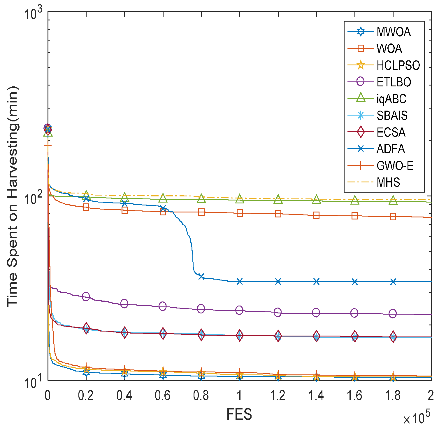
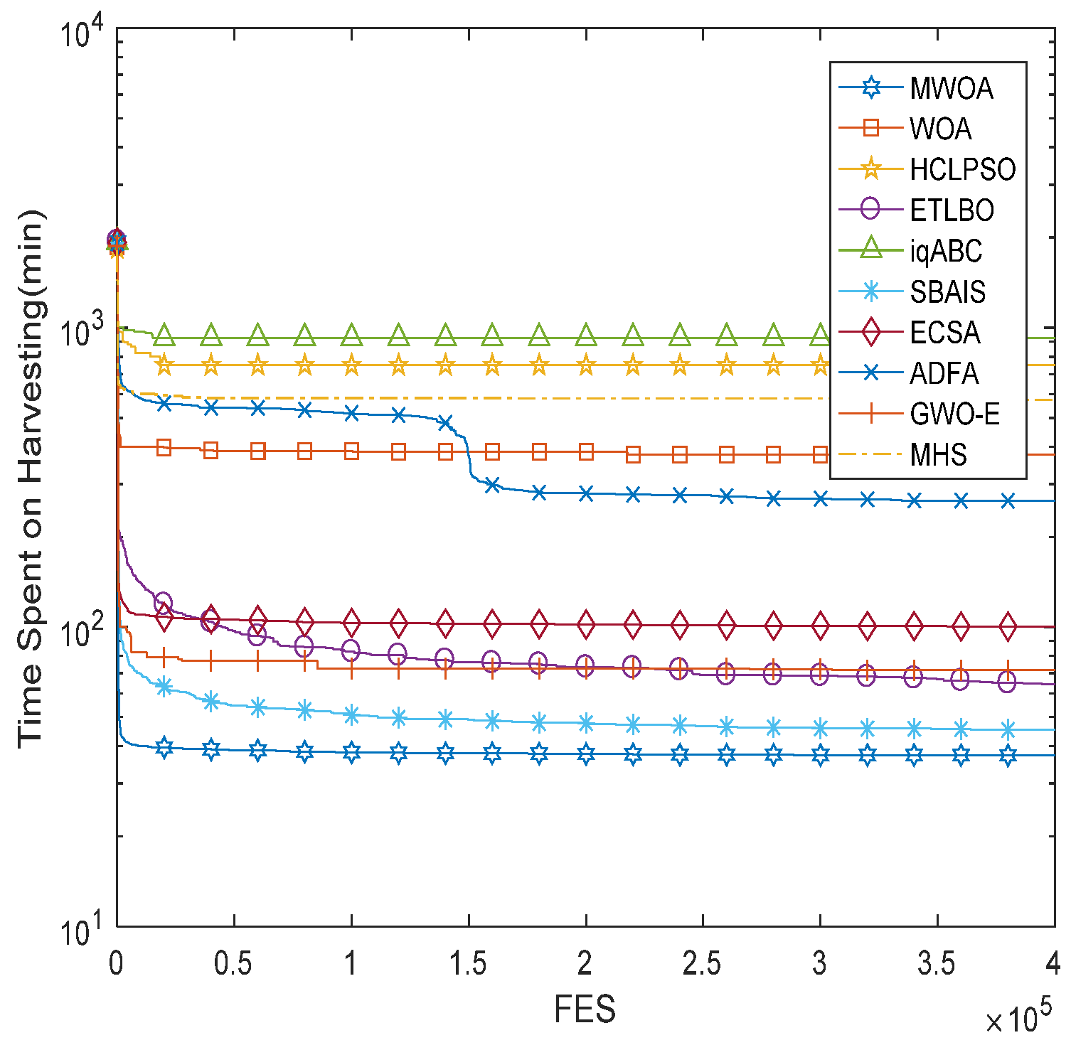
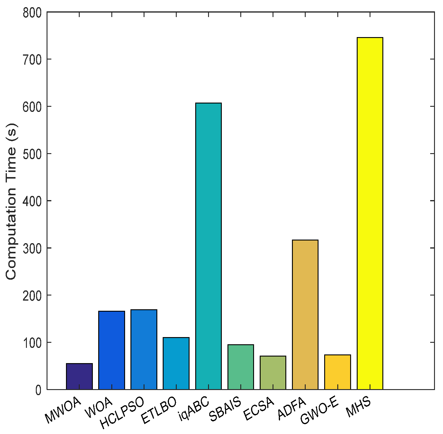
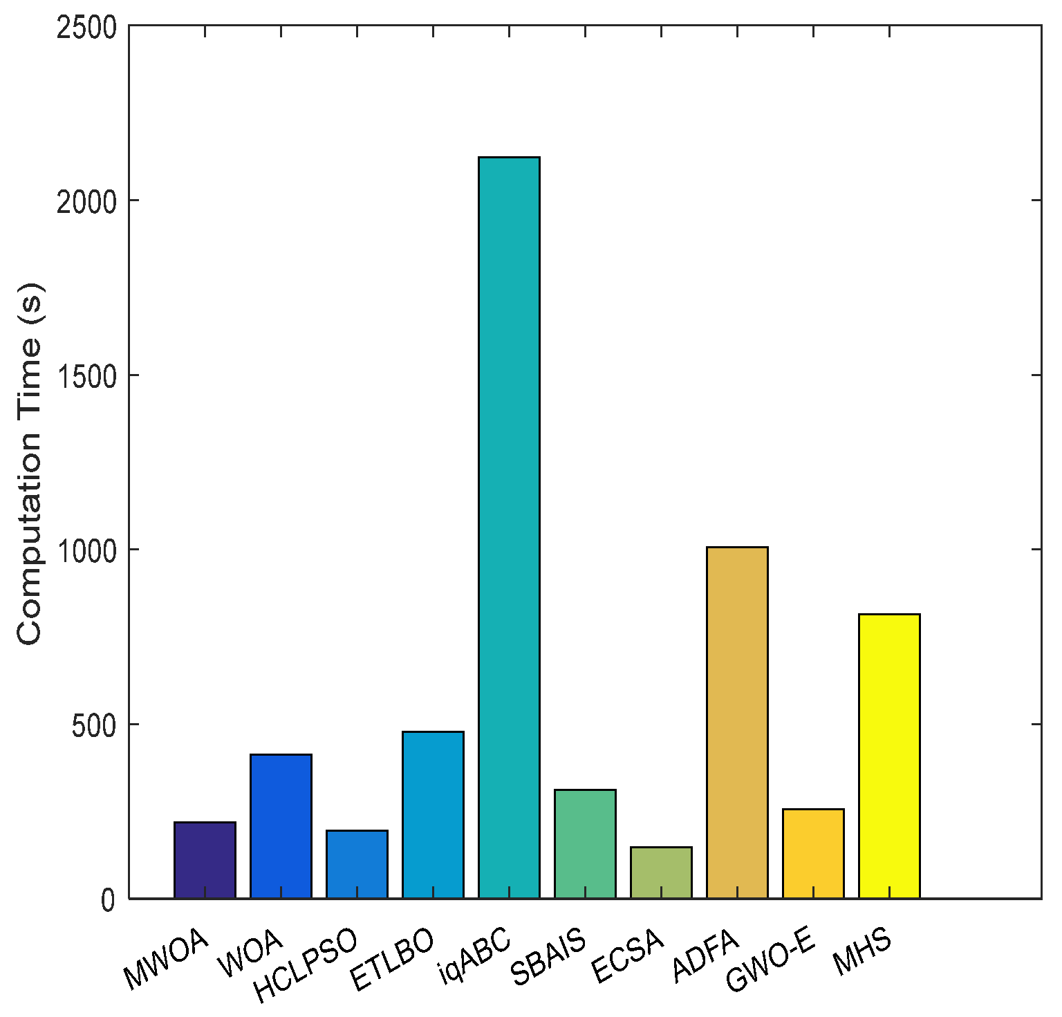
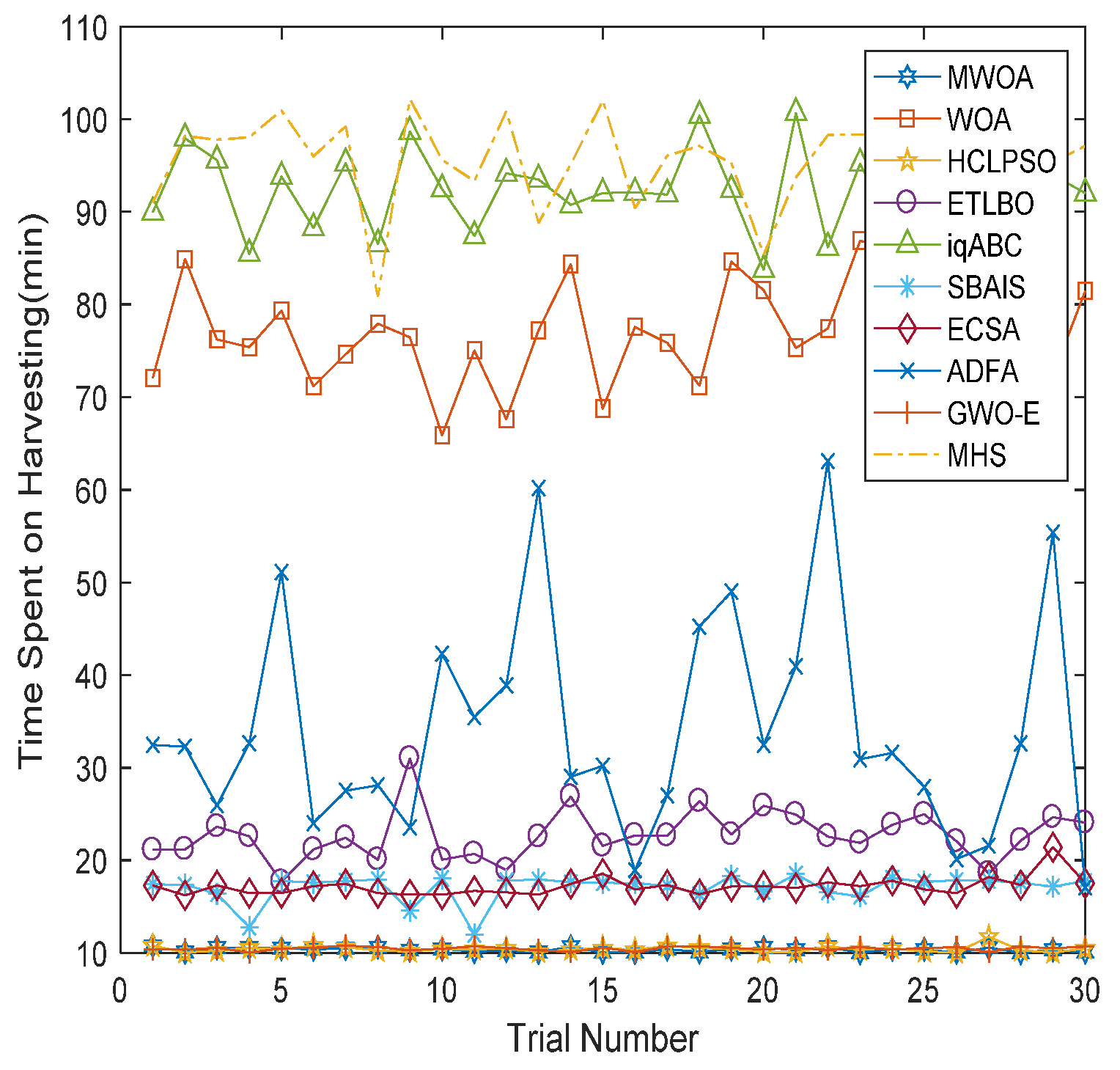
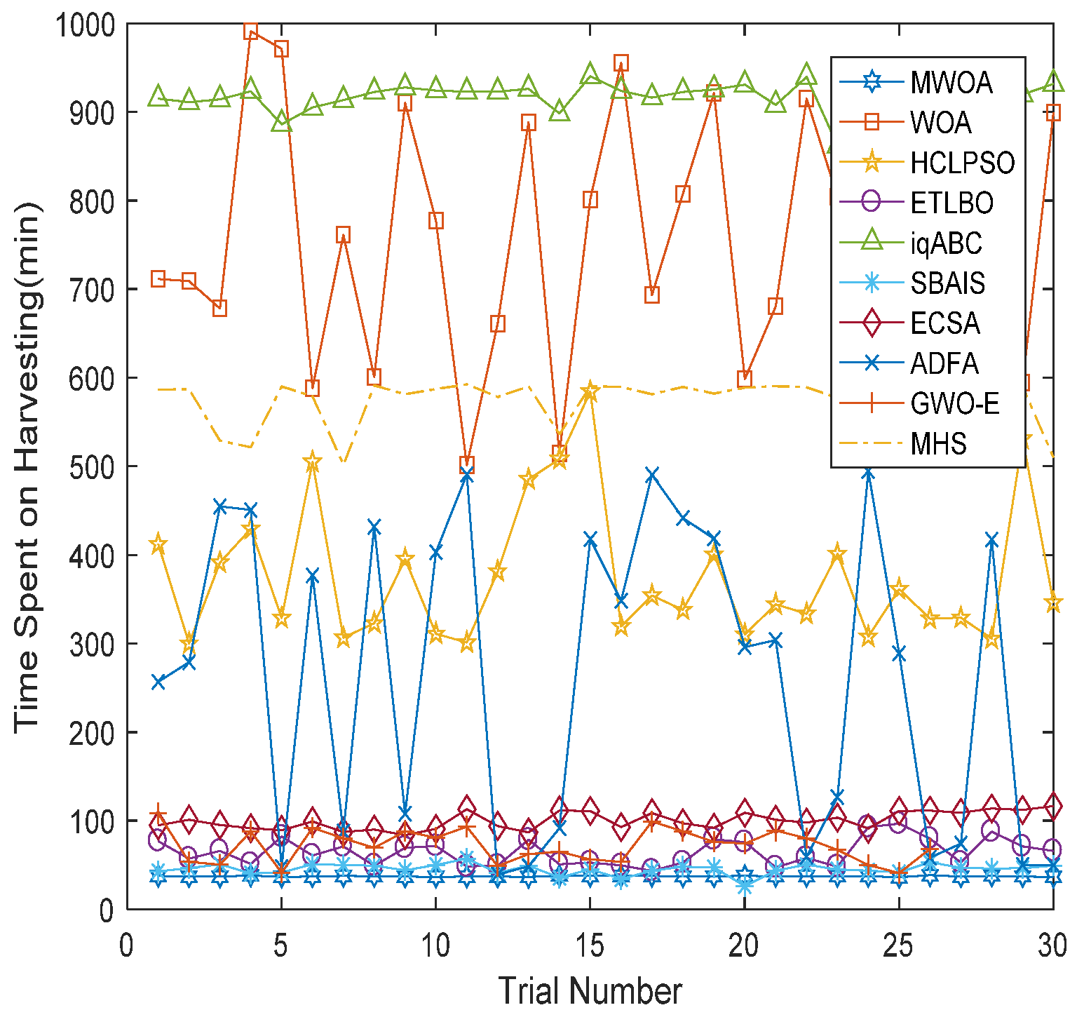
This paper established a model for multi-type harvesters scheduling, and the problem was solved by a proposed meta-heuristic method called the MWOA. The MWOA was realized by making some improvements to the conventional WOA. An opposition-based learning search operator and an adaptive convergence factor were added to the WOA to improve the global convergence and the balance against local convergence. In addition, by using heuristic mutation, the parents whose offspring were trapped in local optima could provide helpful information leading to a promising search, and thus the variety in the population and the ability of the MWOA algorithm to escape from a local optimum were effectively improved. Finally, the numerical simulation results showed that MWOA had better performance in terms of solution quality and convergence speed compared with other swarm-based algorithms for solving the multi-type harvesters scheduling problem.
With the fast development of agricultural collectives, intelligent scheduling of agricultural machinery plays a very important role in maximizing user revenue. Furthermore, the country’s increasing emphasis on environmental protection, energy saving and emission reduction targets, promotes the ability of electric agricultural machinery to gradually enter the market. Cooperation scheduling between diesel agricultural machinery and electric agricultural machinery may lead to future work. Furthermore, to highlight the flexibility and increase realism, complicated harvesters scheduling problems considering refueling, recharging and breakdown should also be investigated.

Author Contributions

Conceptualization, Z.Y. and Y.C.; methodology, Z.Y.; software, W.Y.; validation, W.Y. and Y.C.; formal analysis, Y.C.; investigation, W.Y.; resources, Z.P.; data curation, W.Y.; writing—original draft preparation, W.Y.; writing—review and editing, Z.Y.; visualization, Z.P.; supervision, Y.C.; project administration, Z.P.; funding acquisition, Z.Y. and Y.C. All authors have read and agreed to the published version of the manuscript.

Funding

This research was funded by the National Natural Science Foundation of China (61773156), and the Scientific and Technological Project of Henan (202102110281, 202102110282).

Data Availability Statement

Reasonable requests to access the datasets should be directed to zl.yang@siat.ac.cn.

Conflicts of Interest

The authors declare no conflict of interest.

References

  1. Parray, R.A.; Mani, I.; Kumar, A.; Khura, T.K. Development of web-based combine harvester custom-hiring model for rice-wheat cropping system. Curr. Sci. 2019, 116, 108–111. [Google Scholar] [CrossRef]
  2. Nik, M.A.E.; Khademolhosseini, N.; Abbaspour-Fard, M.H.; Mahdinia, A.; Alami-Saied, K. Optimum utilization of low-capacity combine harvesters in high-yielding wheat farms using multi-criteria decision making. Biosyst. Eng. 2009, 103, 382–388. [Google Scholar] [CrossRef]
  3. Zhang, X.; Wang, L.; Xiong, Q. The shortest path design of combine harvester-based on tabu search and PID algorithm. J. Agric. Mech. Res. 2017, 39, 53–57. [Google Scholar]
  4. Rahman, M.M.; Ishii, K.; Noguchi, N. Optimum harvesting area of convex and concave polygon field for path planning of robot combine harvester. Intell. Serv. Robot. 2019, 12, 167–179. [Google Scholar] [CrossRef] [Green Version]
  5. Willigenburg, L.G.V.; Hol, C.W.J.; Henten, E.J.V. On-line near minimum-time path planning and control of an industrial robot for picking fruits. Comput. Electron. Agric. 2004, 44, 223–237. [Google Scholar] [CrossRef]
  6. Saito, M.; Tamaki, K.; Nishiwaki, K. Development of robot combine harvester for beans using CAN bus network. Proc. IFAC 2013, 46, 148–153. [Google Scholar] [CrossRef]
  7. Sethanan, K.; Neungmatcha, W. Multi-objective Particle Swarm optimization for mechanical harvester route planning of sugarcane field operations. Eur. J. Oper. Res. 2016, 252, 969–984. [Google Scholar] [CrossRef]
  8. Zhang, F.; Teng, G.; Yuan, Y.; Wang, K.; Fan, T.; Zhang, Y. Suitability selection of emergency scheduling and allocating algorithm of agricultural machinery. Trans. Chin. Soc. Agric. Eng. 2018, 34, 47–53. [Google Scholar]
  9. Cao, R.; Li, S.; Ji, Y.; Xu, H.; Zhang, M.; Li, M. Multi-machine cooperation task planning based on ant colony algorithm. Trans. Chin. Soc. Agric. Mach. 2019, 50, 34–39. [Google Scholar]
  10. Lu, E.; Xu, L.z.; Li, Y.M.; Tang, Z.; Ma, Z. Modeling of working environment and coverage path planning method of combine harvesters. Int. J. Agric. Biol. Eng. 2020, 13, 132–137. [Google Scholar] [CrossRef] [Green Version]
  11. Hameed, I.A. Intelligent coverage path planning for agricultural robots and autonomous machines on three-dimensional terrain. Int. J. Intell. Robot. Syst. 2014, 74, 965–983. [Google Scholar] [CrossRef] [Green Version]
  12. Cui, J.; Zhang, X.; Fan, X.; Feng, W.; Wu, Y. Path planning of autonomous agricultural machineries in complex rural road. Int. J. Eng. 2020, 2020, 239–245. [Google Scholar]
  13. Bochtis, D.; Griepentrog, H.W.; Vougioukas, S.; Busato, P.; Berruto, R.; Zhou, K. Route planning for orchard operations. Comput. Electron. Agric. 2015, 113, 51–60. [Google Scholar] [CrossRef]
  14. Zhao, Y.; Zhang, H. Application of machine learning and rule scheduling in a job-shop production control system. Int. J. Simul. Model. 2021, 20, 410–421. [Google Scholar] [CrossRef]
  15. Duplakova, D.; Teliskova, M.; Duplak, J.; Torok, J.; Hatala, M.; Steranka, J.; Radchenko, S. Determination of optimal production process using scheduling and simulation software. Int. J. Simul. Model. 2018, 17, 609–622. [Google Scholar] [CrossRef]
  16. Vázquez-Serrano, J.I.; Cárdenas-Barrón, J.E.; Peimbert-García, R.E. Agent scheduling in unrelated parallel machines with sequence and agent machine dependent setup time problem. Mathematics 2021, 9, 2955. [Google Scholar] [CrossRef]
  17. Zheng, X.; Su, X. Sliding mode control of electro-hydraulic servo system based on optimization of quantum particle swarm algorithm. Machines 2021, 9, 283. [Google Scholar] [CrossRef]
  18. Chu, Z.; Wang, D.; Meng, F. An adaptive RBF-NMPC architecture for trajectory tracking control of underwater vehicles. Machines 2021, 9, 105. [Google Scholar] [CrossRef]
  19. Padmanaban, B.; Sathiyamoorthy, S. A metaheuristic optimization model for spectral allocation in cognitive networks based on ant colony algorithm (M-ACO). Soft Comput. 2020, 24, 15551–15560. [Google Scholar] [CrossRef]
  20. Yang, Q.; Chen, W.N.; Yu, Z.T.; Gu, T.L.; Li, Y.; Zhang, H.X.; Zhang, J. Adaptive multimodal continuous ant colony optimization. IEEE. Trans. Evol. Comput. 2017, 21, 191–205. [Google Scholar] [CrossRef] [Green Version]
  21. Zhang, S.; Du, H.; Borucki, S.; Jin, S.; Hou, T.; Li, Z. Dual resource constrained flexible job shop scheduling based on improved quantum genetic algorithm. Machines 2021, 9, 108. [Google Scholar] [CrossRef]
  22. Awadallah, M.A.; Al-Betar, M.A.; Bolaji, A.L.; Abu Doush, I.; Hammouri, A.I.; Mafarja, M. Island artificial bee colony for global optimization. Soft Comput. 2020, 24, 13461–13487. [Google Scholar] [CrossRef]
  23. Banharnsakun, A. Artificial bee colony algorithm for content-based image retrieval. Comput. Intell. 2020, 36, 351–367. [Google Scholar] [CrossRef]
  24. Kuntoğlu, M.; Acar, O.; Gupta, M.K.; Sağlam, H.; Sarikaya, M.; Giasin, K.; Pimenov, D.Y. Parametric optimization for cutting forces and material removal rate in the turning of AISI 5140. Machines 2021, 9, 90. [Google Scholar] [CrossRef]
  25. Tang, H.; Xue, F. Cuckoo search algorithm with different distribution strategy. Int. J. Bio-Inspir. Comput. 2019, 13, 234–241. [Google Scholar] [CrossRef]
  26. Bányai, T. Optimization of material supply in smart manufacturing environment: A metaheuristic approach for matrix production. Machines 2021, 9, 220. [Google Scholar] [CrossRef]
  27. Mirjalili, S.; Lewis, A. The whale optimization algorithm. Adv. Eng. Softw. 2016, 95, 51–67. [Google Scholar] [CrossRef]
  28. Ezzeldin, R.M.; Djebedjian, B. Optimal design of water distribution networks using whale optimization algorithm. Urban. Water. J. 2020, 17, 14–22. [Google Scholar] [CrossRef]
  29. Abdel-Basset, M.; El-Shahat, D.; Sangaiah, A.K. A modified nature inspired meta-heuristic whale optimization algorithm for solving 0–1 knapsack problem. Int. J. Mach. Learn. Cybern. 2017, 10, 495–514. [Google Scholar]
  30. Aljarah, I.; Faris, H.; Mirjalili, S. Optimizing connection weights in neural networks using the whale optimization algorithm. Soft Comput. 2016, 22, 1–15. [Google Scholar] [CrossRef]
  31. Reddy, P.D.P.; Reddy, V.C.V.; Manohar, T.G. Whale optimization algorithm for optimal sizing of renewable resources for loss reduction in distribution systems. Renew. Wind. Water. Sol. 2017, 4, 3. [Google Scholar] [CrossRef] [Green Version]
  32. Mafarja, M.M.; Mirjalili, S. Hybrid Whale optimization algorithm with simulated annealing for feature selection. Neurocomputing 2017, 260, 302–312. [Google Scholar] [CrossRef]
  33. Hasanien, H.M. Performance improvement of photovoltaic power systems using an optimal control strategy based on whale optimization algorithm. Electr. Power Syst. Res. 2018, 157, 168–176. [Google Scholar] [CrossRef]
  34. Abdel-Basset, M.; Manogaran, G.; El-Shahat, D.; Mirjalili, S. A hybrid whale optimization algorithm based on local search strategy for the permutation flow shop scheduling problem. Future Gener. Comput. Syst. 2018, 85, 129–145. [Google Scholar] [CrossRef] [Green Version]
  35. Tizhoosh, H.R. Opposition-based learning: A new scheme for machine intelligence. In Proceedings of the International Conference on Intelligent Agents, Web Technologies and Internet Commerce, Washington, DC, USA, 28–30 November 2005; pp. 695–701. [Google Scholar]
  36. Lynn, N.; Suganthan, P.N. Heterogeneous comprehensive learning particle swarm optimization with enhanced exploration and exploitation. Swarm. Evol. Comput. 2015, 24, 11–24. [Google Scholar] [CrossRef]
  37. Ramadan, A.; Kamel, S.; Korashy, A.; Yu, J. Photovoltaic cells parameter estimation using an enhanced teaching learning-based optimization algorithm. Iranian J. Sci. Technol. Trans. Elect. Eng. 2020, 44, 767–779. [Google Scholar] [CrossRef]
  38. Aslan, S.; Badem, H.; Karabiga, D. Improved quick artificial bee colony (iqABC) algorithm for global optimization. Soft Comput. 2019, 23, 13161–13182. [Google Scholar] [CrossRef]
  39. Chaudhary, R.; Banati, H. Swarm bat algorithm with improved search (SBAIS). Soft Comput. 2018, 23, 11461–11491. [Google Scholar] [CrossRef]
  40. Nguyen, T.T.; Nguyen, T.T.; Vo, D.N. An effective cuckoo search algorithm for large-scale combined heat and power economic dispatch problem. Neural. Comput. Appl. 2018, 30, 3545–3564. [Google Scholar] [CrossRef]
  41. Suresh, V.; Sreejith, S.; Sudabattula, S.K.; Kamboj, V.K. Demand response-integrated economic dispatch incorporating renewable energy sources using ameliorated dragonfly algorithm. Electr. Eng. 2019, 101, 421–442. [Google Scholar] [CrossRef]
  42. Salgotra, R.; Singh, U.; Sharma, S. On the improvement in grey wolf optimization. Neural. Comput. Appl. 2020, 32, 3709–3748. [Google Scholar] [CrossRef]
  43. Elattar, E.E. Modified harmony search algorithm for combined economic emission dispatch of microgrid incorporating renewable sources. Energy 2018, 159, 496–507. [Google Scholar] [CrossRef]
Figure 1. The principle of multi-type combine harvesters scheduling.
Machines 10 00064 g001
Figure 2. Bubble-net foraging behavior of humpback whale.
Machines 10 00064 g002
Figure 3. Flowchart of WOA.
Machines 10 00064 g003
Figure 4. Mean convergence characteristics of algorithms.
Machines 10 00064 g004aMachines 10 00064 g004b
Figure 5. Mean convergence in 60-field case.
Machines 10 00064 g005
Figure 6. Mean convergence for 120-field case.
Machines 10 00064 g006
Figure 7. Computation times for 60-field case.
Machines 10 00064 g007
Figure 8. Computation times for 120-field case.
Machines 10 00064 g008
Figure 9. Comparisons of each trial for 60-field case.
Machines 10 00064 g009
Figure 10. Comparisons of each trial for 120-field case.
Machines 10 00064 g010
Figure 11. Comparison of harvesting times for 60-field case.
Machines 10 00064 g011
Figure 12. Comparison of harvesting times for 120-field case.
Machines 10 00064 g012
Table 1. Details of benchmark functions.
NameFunctionCSearch RangeMin
Sphere f 1 ( x ) = i = 1 D x i 2 US[−100, 100]0
Sumsquare f 2 ( x ) = i = 1 D i x i 2 US[−10, 10]0
Schwefel2.21 f 3 ( x ) = max { | x i | , 1 x i D } UN[−100, 100]0
Schwefel2.22 f 4 ( x ) = i = 1 D | x i | + i = 1 D | x i | UN[−10, 10]0
Rosenbrock f 5 ( x ) = i = 1 D 1 { 100 ( x i + 1 x i 2 ) 2 + ( 1 x i ) 2 } UN[−5, 10]0
Rastrigin f 6 ( x ) = i = 1 D [ x i 2 10 cos ( 2 π x i ) ] + 10 D MS[−5.12, 5.12]0
Ackley f 7 ( x ) = 20 exp ( 0.2 1 D i = 1 D x i 2 ) exp ( 1 D i = 1 D cos ( 2 π x i ) ) + 20 + e MN[−32, 32]0
Levy f 8 ( x ) = i = 1 D 1 ( x i 1 ) 2 [ 1 + sin 2 ( 3 π x i + 1 ) ] + sin 2 ( 3 π x 1 ) + | x D 1 | [ 1 + sin 2 ( 3 π x D ) ] MN[−10, 10]0
Table 2. Comparison of results for 30-dimension benchmark functions.
Algorithm f1f2f3f4f5f6f7f8
MWOAMean2.17 × 10−2704.90 × 10−2811.41 × 10−44.40 × 10−178003.61 × 10−157.59 × 10⁻²⁸
Std006.98 × 10−40002.41 × 10−152.33 × 10⁻²⁷
WOAMean6.69 × 10−1121.12 × 10−1212.03 × 10−14.62 × 10−892.59 × 1011.89 × 10−153.97 × 10−151.17 × 10⁻¹
Std2.16 × 10−1215.91 × 10−1213.48 × 10−11.47 × 10−883.67 × 10−11.04 × 10−142.76 × 10−156.24 × 10⁻²
Sig++++++=+
HCLPSOMean4.47 × 10−265.96 × 10−281.15 × 10−13.29 × 10−142.10 × 1012.243.93 × 10−135.78 × 10⁻¹
Std2.22 × 10−251.04 × 10−276.26 × 10−29.68 × 10−142.91 × 1011.074.18 × 10−134.11 × 10⁻¹
Sig++++++++
ETLBOMean4.80 × 10−295.02 × 10−302.55 × 1012.757.85 × 1011.52 × 1022.923.39 × 101
Std4.83 × 10−293.64 × 10−302.812.329.07 × 1011.19 × 1022.003.20
Sig++++++++
iqABCMean4.10 × 10−141.77 × 10−141.30 × 1012.58 × 10−147.18 × 10−13.48 × 10−35.69 × 10−104.93 × 10⁻¹⁰
Std4.18 × 10−141.69 × 10−142.022.20 × 10−144.67 × 10−11.32 × 10−28.30 × 10−107.84 × 10⁻¹⁰
Sig++++++++
SBAISMean1.75 × 1015.80 × 10−11.024.15 × 10−11.25 × 10−24.04 × 10−12.185.95 × 10−1
Std4.02 × 1016.91 × 10−18.62 × 10−15.55 × 10−11.18 × 10−24.25 × 10−11.862.97 × 10−1
Sig++++++++
ECSAMean2.10 × 1041.62 × 1035.23 × 1012.48 × 1097.68 × 1041.70 × 1021.54 × 1011.58 × 102
Std7.45 × 1036.64 × 1021.22 × 1013.50 × 1095.69 × 1044.71 × 1019.20 × 10−16.09 × 101
Sig++++++++
ADFAMean2.524.25 × 1014.268.741.94 × 1021.10 × 1022.906.90
Std5.92 × 10−12.52 × 1016.554.907.89 × 1015.82 × 1013.43 × 10−14.32
Sig++++++++
GWO-EMean1.50 × 10−438.81 × 10−461.381.05 × 10−277.127.77 × 10−11.06 × 10−147.12
Std8.20 × 10−434.55 × 10−451.913.38 × 10−271.06 × 1013.313.95 × 10−152.93
Sig++++++++
MHSMean3.45 × 1044.63 × 1036.63 × 1012.09 × 1063.15 × 1053.21 × 1021.95 × 1015.12 × 102
Std2.73 × 1034.25 × 1022.093.26 × 1066.13 × 1041.06 × 1011.63 × 10−16.27 × 101
Sig++++++++
The best results are highlighted in boldface.
Table 3. Comparison of results for 50-dimension benchmark functions.
Algorithm f1f2f3f4f5f6f7f8
MWOAMean9.88 × 10−3247.91 × 10−3239.79 × 10−13.95 × 10−219003.26 × 10−153.93 × 10⁻¹⁸
Std001.160002.35 × 10−151.36 × 10⁻¹⁷
WOAMean8.09 × 10−1526.44 × 10−1531.731.55 × 10−1064.59 × 1013.79 × 10−153.38 × 10−152.53 × 10⁻¹
Std3.50 × 10−1512.53 × 10−1522.198.46 × 10−1062.90 × 10−12.08 × 10−142.31 × 10−152.01 × 10⁻¹
Sig++=+++=+
HCLPSOMean2.52 × 10−175.45 × 10−191.854.64 × 10−104.13 × 1011.00 × 1012.79 × 10−94.45 × 10⁻¹
Std9.32 × 10−177.43 × 10−195.67 × 10−17.17 × 10−104.26 × 1013.112.49 × 10−92.27 × 10⁻¹
Sig++++++++
ETLBOMean1.21 × 10−283.54 × 10−293.13 × 1013.643.30 × 1022.17 × 1023.156.38 × 101
Std8.70 × 10−294.27 × 10−299.753.909.45 × 1022.12 × 1022.631.54 × 101
Sig++++++++
iqABCMean4.02 × 10−131.61 × 10−132.68 × 1012.25 × 10−131.179.97 × 10−21.38 × 10−81.87 × 10−9
Std4.41 × 10−131.78 × 10−133.174.46 × 10−138.91 × 10−11.66 × 10−13.22 × 10−82.86 × 10−9
Sig++++++++
SBAISMean4.471.39 × 10−13.193.07 × 10−12.36 × 10−21.163.041.41
Std8.302.85 × 10−13.183.94 × 10−12.47 × 10−29.86 × 10−13.257.52 × 10−1
Sig++++++++
ECSAMean2.00 × 1046.59 × 1035.67 × 1016.39 × 1093.61 × 1053.19 × 1021.62 × 1013.39 × 102
Std4.56 × 1031.74 × 1038.774.68 × 1091.58 × 1058.45 × 1011.139.83 × 101
Sig++++++++
ADFAMean7.591.54 × 1021.28 × 1011.49 × 1014.73 × 1021.87 × 1024.161.00 × 101
Std1.201.03 × 1029.688.203.27 × 1028.59 × 1011.373.82
Sig++++++++
GWO-EMean4.31 × 10−461.31 × 10−461.532.36 × 10−314.431.89 × 10−151.07 × 10−141.05 × 101
Std1.76 × 10−455.95 × 10−464.517.28 × 10−318.971.04 × 10−143.19 × 10−155.89
Sig++++++++
MHSMean8.45 × 1041.82 × 1047.93 × 1012.62 × 10161.27 × 1066.10 × 1022.01 × 1011.25 × 103
Std4.56 × 1031.22 × 1032.645.22 × 10161.64 × 1051.40 × 1011.14 × 10−16.09 × 101
Sig++++++++
The best results are highlighted in boldface.
Table 4. Comparison of results for 100-dimension benchmark functions.
Algorithm f1f2f3f4f5f6f7f8
MWOAMean001.340002.90 × 10−156.81 × 10⁻²¹
Std001.550002.41 × 10−153.68 × 10⁻²⁰
WOAMean01.98 × 10−3231.457.38 × 10−3209.49 × 10108.82 × 10−151.88 × 10⁻¹
Std001.7902.80 × 10−103.58 × 10−151.64 × 10⁻¹
Sig=+=++=++
HCLPSOMean1.03 × 10−224.48 × 10−233.324.60 × 10−134.90 × 1011.39 × 1019.27 × 10−152.67 × 10⁻¹
Std1.07 × 10−224.42 × 10−234.79 × 10−15.13 × 10−134.93 × 1013.326.82 × 10−121.44 × 10⁻¹
Sig++++++++
ETLBOMean2.47 × 10−281.93 × 10−285.51 × 1015.892.54 × 1021.19 × 1022.301.12 × 102
Std2.14 × 10−282.22 × 10−282.17 × 1018.012.36 × 1022.50 × 1022.181.14 × 101
Sig++++++++
iqABCMean1.68 × 10−111.02 × 10−113.86 × 1015.98 × 10−121.909.33 × 10−23.76 × 10−76.95 × 10−9
Std3.10 × 10−119.24 × 10−124.219.20 × 10−121.501.01 × 10−14.98 × 10−79.84 × 10−9
Sig++++++++
SBAISMean1.13 × 1011.14 × 10−12.563.63 × 10−19.32 × 10−32.403.621.01
Std1.62 × 1017.11 × 10−31.804.65 × 10−19.56 × 10−31.232.187.67 × 10−1
Sig++++++++
ECSAMean5.17 × 1042.31 × 1046.85 × 1013.00 × 10181.03 × 1067.34 × 1021.73 × 1018.61 × 102
Std1.72 × 1046.39 × 1037.231.64 × 10192.68 × 1051.32 × 1027.06 × 10−12.03 × 10²
Sig++++++++
ADFAMean2.75 × 1015.01 × 1021.51 × 1012.14 × 1015.13 × 1021.50 × 1024.972.27 × 101
Std2.674.87 × 1027.721.70 × 1016.63 × 1021.15 × 1022.091.32 × 101
Sig++++++++
GWO-EMean1.37 × 10−1321.19 × 10−1324.883.00 × 10−851.3104.56 × 10−151.72 × 101
Std5.92 × 10−1326.51 × 10−1328.731.02 × 10−841.3902.55 × 10−151.17 × 101
Sig++++++++
MHSMean2.04 × 1059.33 × 1048.82 × 1018.25 × 10384.59 × 1061.39 × 1032.05 × 1012.94 × 103
Std4.21 × 1033.93 × 1031.221.92 × 10393.18 × 1052.35 × 1015.35 × 10−27.14 × 101
Sig++++++++
The best results are highlighted in boldface.
Table 5. The basic parameters of various types of harvesters.
ParameterType of Harvester
Type 1Type 2Type 3Type 4Type 5Type 6
Travel speed25 km/h30 km/h35 km/h40 km/h45 km/h50 km/h
Harvesting speed15 km/h20 km/h25 km/h30 km/h35 km/h40 km/h
Header width1.5 m2 m2.5 m3 m3.5 m4 m
Table 6. The detailed information for 60 fields.
No.Size (m)Cdnt (m)No.Size (m)Cdnt (m)No.Size (m)Cdnt (m)
1(55,10)(75,31)21(9,28)(1193,874)41(75,64)(2429,1929)
2(25,15)(130,41)22(126,81)(1202,902)42(106,314)(2504,1993)
3(51,27)(155,56)23(50,29)(1328,983)43(56,19)(2610,2307)
4(106,25)(206,83)24(69,55)(1378,1012)44(87,64)(2666,2326)
5(95,23)(412,108)25(20,36)(1447,1067)45(49,39)(2753,2390)
6(14,27)(507,131)26(111,77)(1467,1103)46(87,56)(2802,2429)
7(19,20)(521,158)27(136,116)(1578,1180)47(24,15)(2889,2485)
8(37,42)(540,178)28(55,34)(1714,1296)48(38,40)(2913,2500)
9(44,31)(577,220)29(39,27)(1769,1330)49(128,99)(2951,2540)
10(55,55)(621,251)30(18,83)(1808,1357)50(145,176)(3079,2639)
11(33,87)(676,306)31(77,67)(1826,1440)51(141,120)(3224,2815)
12(80,38)(709,393)32(27,33)(1903,1507)52(15,46)(3365,2935)
13(62,38)(789,431)33(15,12)(1930,1540)53(78,39)(3380,2981)
14(50,99)(851,469)34(71,42)(1945,1552)54(104,49)(3458,3020)
15(16,54)(901,568)35(80,89)(2016,1594)55(74,21)(3562,3069)
16(38,80)(917,622)36(37,16)(2096,1683)56(69,76)(3636,3090)
17(67,48)(955,702)37(64,35)(2133,1699)57(89,61)(3705,3166)
18(80,60)(1022,750)38(38,68)(2197,1734)58(94,37)(3794,3227)
19(43,37)(1102,810)39(158,76)(2235,1802)59(98,77)(3888,3264)
20(48,27)(1145,847)40(36,51)(2393,1878)60(99,97)(3986,3341)
Table 7. Comparison of results for 60-field case.
MinMaxMeanStdSig
MWOA1.00 × 1011.08 × 1011.03 × 1012.00 × 10−1/
WOA6.59 × 1018.69 × 1017.65 × 1015.64+
HCLPSO1.00 × 1011.18 × 1011.04 × 1013.40 × 10−1=
ETLBO1.77 × 1013.10 × 1012.27 × 1012.70+
iqABC8.37 × 1011.01 × 1029.25 × 1014.44+
SBAIS1.20 × 1011.85 × 1011.71 × 1011.50+
ECSA1.62 × 1012.14 × 1011.72 × 1019.92 × 10−1+
ADFA1.71 × 1016.31 × 1013.43 × 1011.19 × 101+
GWO-E1.00 × 1011.10 × 1011.05 × 1012.23 × 10−1+
MHS8.08 × 1011.02 × 1029.54 × 1014.76+
The best results are highlighted in boldface.
Table 8. Comparison of results for 120-field case.
MinMaxMeanStdSig
MWOA3.61 × 1013.84 × 1013.73 × 1014.95 × 10−1/
WOA3.00 × 1025.84 × 1023.76 × 1027.71 × 101+
HCLPSO5.01 × 1029.91 × 1027.49 × 1021.44 × 102+
ETLBO4.35 × 1019.68 × 1016.45 × 1011.51 × 101+
iqABC9.22 × 1029.27 × 1029.24 × 1023.60+
SBAIS2.62 × 1015.70 × 1014.53 × 1016.05+
ECSA8.36 × 1011.16 × 1021.00 × 1029.81+
ADFA3.94 × 1014.94 × 1022.63 × 1021.72 × 102+
GWO-E4.11 × 1011.08 × 1027.17 × 1011.86 × 101+
MHS5.02 × 1015.93 × 1025.74 × 1022.67 × 101+
The best results are highlighted in boldface.
Publisher’s Note: MDPI stays neutral with regard to jurisdictional claims in published maps and institutional affiliations.

