Value at Risk Based on Fuzzy Numbers ^†

Abstract

Value at Risk (VaR) has become a crucial measure for decision making in risk management over the last thirty years and many estimation methodologies address the finding of the best performing measure at taking into account unremovable uncertainty of real financial markets. One possible and promising way to include uncertainty is to refer to the mathematics of fuzzy numbers and to its rigorous methodologies which offer flexible ways to read and to interpret properties of real data which may arise in many areas. The paper aims to show the effectiveness of two distinguished models to account for uncertainty in VaR computation; initially, following a non parametric approach, we apply the Fuzzy-transform approximation function to smooth data by capturing fundamental patterns before computing VaR. As a second model, we apply the Average Cumulative Function (ACF) to deduce the quantile function at point p as the potential loss VaR${}_p$ for a fixed time horizon for the 100p% of the values. In both cases a comparison is conducted with respect to the identification of VaR through historical simulation: twelve years of daily S&P500 index returns are considered and a back testing procedure is applied to verify the number of bad VaR forecasting in each methodology. Despite the preliminary nature of the research, we point out that VaR estimation, when modelling uncertainty through fuzzy numbers, outperforms the traditional VaR in the sense that it is the closest to the right amount of capital to allocate in order to cover future losses in normal market conditions.

1. Introduction

In 1996 the Basel Committee approved the use of proprietary Value at Risk (VaR) measures for calculating the market risk component of bank capital requirements; from that year, the scientific literature grew dramatically in order to identify the best performing way to measure VaR.

Jorion in [1] defines VaR as the measure that is the worst expected loss over a given horizon under normal market conditions at a given level of confidence. When a bank says that the daily VaR of its trading portfolio is $1 million at the 95 percent confidence level, it means if no negative event occurs, while only five percent of the time, the daily loss will exceed $1 million. The VaR is thus a conditional quantile of the asset return loss distribution.

Despite the VaR is an intuitive concept, its computation may be complex; a detailed review about the classical methodologies is in [2] where they are classified into three sets (i) the variance–covariance approach, also called the Parametric method, (ii) the Historical Simulation (Non-parametric method) and (iii) the Monte Carlo simulation, which is a Semi-parametric method. In the first papers based on the comparison between the three approaches, no methodology seemed to perform better than the others. However, more recently some contributions report that the Historical Simulation produces almost poor VaR estimates basically because it does not offer an efficient use of the available information.

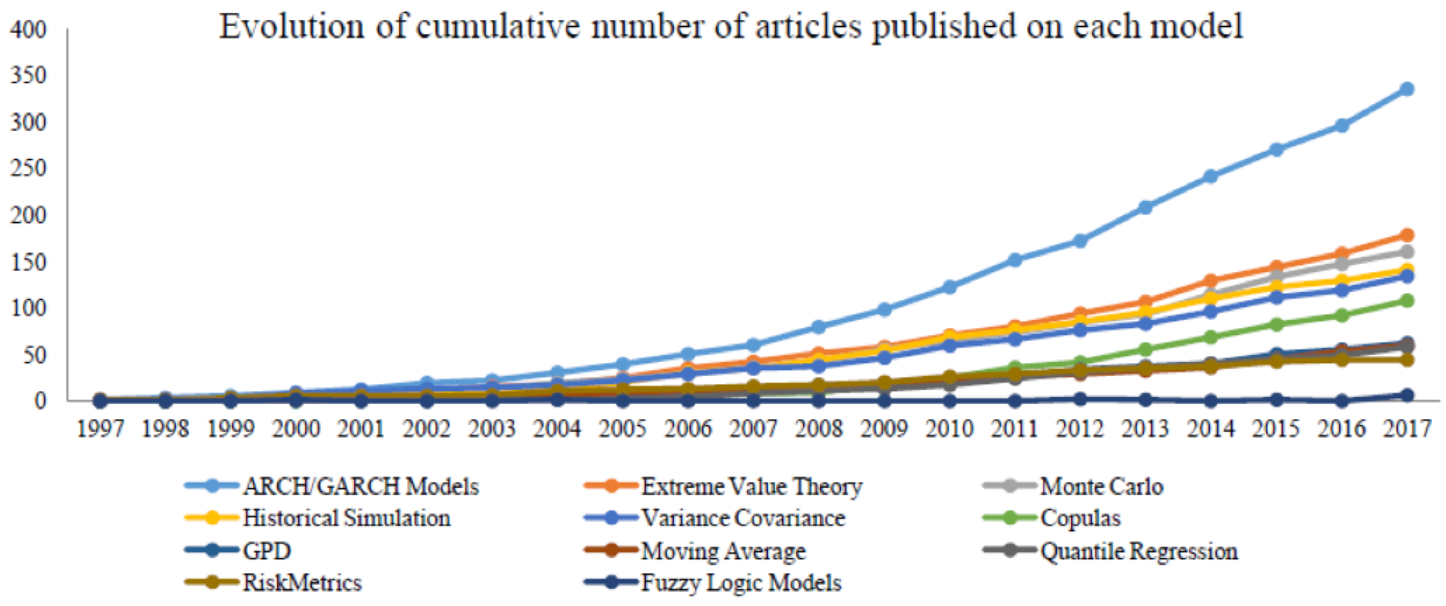
A more recent review, presented in [3], concerns studies for VaR computations including several approaches, related literature is relatively scarce, developed when uncertainty modeling is based on fuzzy logic; the authors show in Figure 1 the amount of articles within each methodology in a time period of twenty years.

About twenty years ago, the first attempt to apply Fuzzy Logic in the estimation of VaR was shown in [4] where market liquidity is a key factor in the definition of a pricing model through a fuzzy measure.

Fuzzy numbers describe the implicit vagueness within VaR in [5]; they play the role of a sensitivity analysis while the stochastic nature of the risky component is preserved.

In [6] interval estimation of VaR values are the input variables of a Fuzzy Slack-Based Measurement that is useful for representing the implications of risk and the effects of risk on efficiency.

The situation of leptokurtic and imprecise risk factors modelled as fuzzy random variables, generalizing [7], is analyzed in Reference [8] where linear portfolio VaR and expected shortfall (ES) are computed. The models imply the possibility of taking into account pessimistic or optimistic investor’s believes.

In [9] VaR is estimated by using probabilistic fuzzy systems (PFSs) which are semi-parametric methods that combines a linguistic description of the system behavior with statistical properties of the data; the approach to designing probabilistic fuzzy VaR models is compared with GARCH model and statistical back testing always accepts PFS models after tuning, whereas GARCH models may be rejected in some situations.

A possibilistic portfolio model is proposed in [10] as an expansion of the possibilistic mean-variance model by with VaR constraint and risk-free investment are computed taking the assumption that the expected rate of returns is a fuzzy number. In [11] the authors suggest an evolving possibilistic fuzzy modeling (ePFM) approach to estimate VaR; data from the main global equity market indexes are used to estimate VaR using ePFM and the performance of ePFM is compared with traditional VaR benchmarks producing encouraging results. A growing interest for researches and practitioners is directed to VaR estimation in the case of operational risk, in [12] the intrinsic properties of the data as fuzzy sets are related to the linguistic variables of the observed data (external), allowing an organization to supervise operational VaR over time.

The notion of credibilistic average VaR is detailed in [13] where simulation algorithms support its use in many real problems of risk analysis.

An alternative nonparametric approach based on maxitive kernel estimation of VaR is studied in [14] where the obtained interval-valued VaR estimates are the key factors to lead to accurate decisions involving uncertainty.

Nevertheless, we believe that the modeling of uncertainty through fuzzy logic in decision making and risk management deserves in-depth analysis; just to mention some of our contributions, we developed the rigorous use of the extension principle for fuzzy-valued functions in [15] where we show that fuzzy financial option prices can capture the unavoidable uncertainty of several stylized facts in real markets and the subjective believes of the investor. It is a matter of interest the use of VaR as a factor fixing decision-making believes for risk-averse investors, for example in [16], the process of recovering investment opportunities with projects that have been rejected when applying the criterion of the Value-at-Risk method, is studied.

In [17] we took three financial time series and we modeled them with two non-parametric smoothing techniques defined in terms of expectile and quantile fuzzy-valued Fuzzy-transform, respectively obtained by minimizing a least squares (L${}_2$-norm) operator and a L${}_1$-norm operator. The relevance of expectiles in risk management is also focused in [18] where it is shown that several limits of VaR and expected shortfall can be overcome by expectiles because they are the only elicitable law-invariant coherent risk measures.

The goal of the present paper is to highlight potentialities of fuzzy numbers in VaR estimation which is a fundamental topic in risk management because the amount of capital to be allocated in case of future losses has to be identified carefully—if it is too small then it does not cover from adverse events and if it is too large then the allocated capital can not be used for other crucial activities. To reach the goal we apply two results which provide instruments for detecting time series properties and for modelling their uncertainty.

The first VaR estimation is produced by the mentioned smoothing techniques, based on Fuzzy-transform and evaluated by performing a rolling window analysis along twelve years of daily returns, during which we count the number of violations and we compare it to the traditional historical simulation.

The second approach addresses non parametric methods and, as in [19], we propose a method to estimate quantiles through a nonparametric estimates of the cumulative distribution function deduced by using the Average Cumulative Function (ACF) which plays the role of the double kernel smoothing in the mentioned paper.

The choice of ACF, introduced in [20] as an alternative representation of fuzzy numbers, is justified in terms of an interesting link which can be established between ACF-representation and quantile functions, without requiring distributional assumptions. In [21] we extend the ACF analysis and in particular we clarify the crucial role of ACF in determining the membership function from experimental data. Again we compare the number of violations when VaR is defined in terms of ACF, with the same number obtained through the historical simulation of VaR.

The paper is organized into seven sections. The second section fixes the basis of the F-transform smoothing techniques that are applied in Section 3 within the case of VaR estimates for daily S&P500 index data, from June 2007 to June 2019. The fourth section gives the basic knowledge of the Average Cumulative Function which allows the interpretation of the fuzzy quantile function in terms of VaR; in Section 5 experiments are given with the same time series as in Section 3, in relation to which the comparison is detailed in Section 6. Highlights on possible future researches are investigated in Section 7.

2. Fuzzy-Transform Smoothing

In [17] two non-parametric smoothing methodologies are introduced; the expectile fuzzy-valued F-transform is based on the classical F-transform obtained by minimizing a least squares ($L_2$-norm) operator, while the quantile fuzzy-valued F-transform is based on the $L_1$-type F-transform, obtained by minimizing an $L_1$-norm operator.

The F-transform smoothing methodologies are compared with:

(1)

expectreg and quantreg package, implemented in R language(CRAN repository);

(2)

SVM-type (Support Vector Machine) non-parametric learning algorithms, implemented in R language (CRAN repository)

Eight measures are checked and they are minimized by both quantile and expectile smoothed series, where quantile performs slightly better for those time series having steep peaks. In addition, the robustness is confirmed within time series of various types. We detail some useful preliminaries explaining the theoretical steps in the discrete case which fits the time series experiments in Section 3.

Given m values $(t_i,f\left(t_i\right))$, $t_i\in [a,b]$, $i=1,\dots ,m$, of a function $f:[a,b]⟶R$, a fuzzy partition $(P,A)$ of $[a,b]$ such that each subinterval $[x_{k-1},x_{k+1}]$ contains at least one point $t_i$ in its interior (so that the basic functions $A_1,\dots ,A_n$ satisfy ${\sum }_{i=1}^m{A}_k\left(t_i\right)>0$ for all k), then the discrete direct F-transform of f with respect to $(P,A)$ is the n-tuple of real numbers $(F_1,\dots ,F_n)$ given by

$$F_k=\frac{{\displaystyle \sum _{i=1}^m}f\left(t_i\right)A_k\left(t_i\right)}{{\displaystyle \sum _{i=1}^m}{A}_k\left(t_i\right)},k=1,\dots ,n,$$

(1)

where $F_k$ minimizes the function

$${\Phi }_{m,k}\left(y\right)=\sum _{i=1}^m{\left|f\left(t_i\right)-y\right|}^2{A}_k\left(t_i\right).$$

(2)

Under certain hypothesis, the minimization of ${\Phi }_{k,\alpha }^{-}\left(\mu \right)$ and ${\Phi }_{k,\alpha }^{+}\left(\mu \right)$ produces two values ${\mu }_{k,\alpha }^{-}$ and ${\mu }_{k,\alpha }^{+}$, for $|\omega \in [0,1]$ that are the (midpoint) minimizers of functions ${\Phi }_{k,\alpha }^{-}\left(\eta \right)$ and ${\Phi }_{k,\alpha }^{+}\left(\eta \right)$; when $\alpha \in [0,1]$ then the compact intervals are defined as:

$$U_{k,\alpha }=\left\{\begin{array}{ccc}\left\{{\mu }_k\left(\frac{1}{2}\right)\right\}\hfill & \mathrm{if}& \alpha =1\\ \left[{\mu }_k\left(\frac{\alpha }{2}\right),{\mu }_k\left(1-\frac{\alpha }{2}\right)\right]\hfill & \mathrm{if}& \alpha \in [0,1]\\ cl\left({\displaystyle \bigcup _{\beta >0}}{U}_{k,\beta }\right)\hfill & \mathrm{if}& \alpha =0\end{array}\right..$$

(3)

Then, for each $k=2-r,\dots ,n+r-1$, the family of intervals $\{U_{k,\alpha };\alpha \in [0,1]\}$ defines the $\alpha$-cuts of a fuzzy number $F_k\in {\mathbb{R}}_{\mathcal{F}}$ having membership function

$$F_k\left(x\right)=\left\{\begin{array}{ccc}sup\left\{\alpha \right|x\in U_{k,\alpha }\}\hfill & \mathrm{if}& x\in U_{k,0}\\ 0\hfill & \mathrm{if}& x\notin U_{k,0}\end{array}\right..$$

(4)

Given a set of m points $Y_m=\{(t_i,f\left(t_i\right));$$i=1,\dots ,m\}$, $t_i\in [a,b]$ of a function $f:[a,b]⟶R$ and given a fuzzy partition $(P,A)$ of $[a,b]$, the (n)-vector of fuzzy numbers

$${\mathbf{F}}_{(\mathbb{P},\mathbb{A})}=(F_1,\dots ,F_n),$$

(5)

where each fuzzy interval $F_k$ has $\alpha$-cuts $U_{k,\alpha }$, is called the discrete direct quantile fuzzy transform of f with respect to $(P,A)$, based on the data-set $Y_m$.

The corresponding inverse expectile fuzzy transform of f is the fuzzy-valued function defined by

$${\widehat{f}}_{(\mathbb{P},\mathbb{A})}\left(x\right)=\sum _{k=1}^n{F}_k{A}_k\left(x\right)\mathrm{for}x\in [a,b].$$

(6)

In the same framework established to deduce (1), the discrete direct F-transform of f with respect to $(\mathbb{P},\mathbb{A})$ is the n-tuple of real numbers $(G_1,\dots ,G_n)$ given by

$$G_k=\frac{{\displaystyle \sum _{i=1}^m}f\left(t_i\right)A_k\left(t_i\right)}{{\displaystyle \sum _{i=1}^m}{A}_k\left(t_i\right)},k=1,\dots ,n$$

(7)

and, in the $L_1$-norm case, each $G_k$ minimizes the function.

$${\Psi }_{m,k}\left(y\right)=\sum _{i=1}^m\left|f\left(t_i\right)-y\right|A_k\left(t_i\right)$$

(8)

Under some hypothesis, the minimization of ${\Psi }_{k,\alpha }^{-}\left(\mu \right)$ and ${\Psi }_{k,\alpha }^{+}\left(\mu \right)$ produces two values ${\eta }_{k,\alpha }^{-}$ and ${\eta }_{k,\alpha }^{+}$, for $|\omega \in [0,1]$ that are the (midpoint) minimizers of functions ${\Psi }_{k,\alpha }^{-}\left(\eta \right)$ and ${\Psi }_{k,\alpha }^{+}\left(\eta \right)$; consider $\alpha \in [0,1],$ the compact intervals

$$V_{k,\alpha }=\left\{\begin{array}{ccc}\left\{{\eta }_k\left(\frac{1}{2}\right)\right\}\hfill & \mathrm{if}& \alpha =1\\ \left[{\eta }_k\left(\frac{\alpha }{2}\right),{\eta }_k\left(1-\frac{\alpha }{2}\right)\right]\hfill & \mathrm{if}& \alpha \in [0,1]\\ cl\left({\displaystyle \bigcup _{\beta >0}}{V}_{\beta }\right)\hfill & \mathrm{if}& \alpha =0;\end{array}\right.$$

(9)

form the $\alpha$-cuts of a fuzzy number $v_k\in {\mathbb{R}}_{\mathcal{F}}$ having membership function

$$v_k\left(x\right)=\left\{\begin{array}{ccc}sup\left\{\alpha \right|x\in V_{k,\alpha }\}\hfill & \mathrm{if}& x\in V_{k,0}\\ 0\hfill & \mathrm{if}& x\notin V_{k,0}.\end{array}\right.$$

(10)

Given a set of m points $Y_m=\{(t_i,f\left(t_i\right));$$i=1,\dots ,m\}$, $t_i\in [a,b]$, of a function $f:[a,b]⟶R$ and given a fuzzy partition $(P,A)$ of $[a,b]$, the (n)-vector of fuzzy numbers

$${\mathbf{G}}_{(\mathbb{P},\mathbb{A})}=(G_1,\dots ,G_n),$$

(11)

where each fuzzy interval $G_k$ has $\alpha$-cuts $V_{k,\alpha }$, is called the discrete direct quantile fuzzy transform of f with respect to $(P,A)$, based on the data-set $Y_m$.

The corresponding inverse quantile fuzzy transform of f is the fuzzy-valued function defined by

$${\tilde{f}}_{(\mathbb{P},\mathbb{A})}\left(x\right)=\frac{1}{r}\sum _{k=1}^n{G}_k{A}_k\left(x\right)\mathrm{for}x\in [a,b].$$

(12)

3. Value at Risk through Smoothed Series

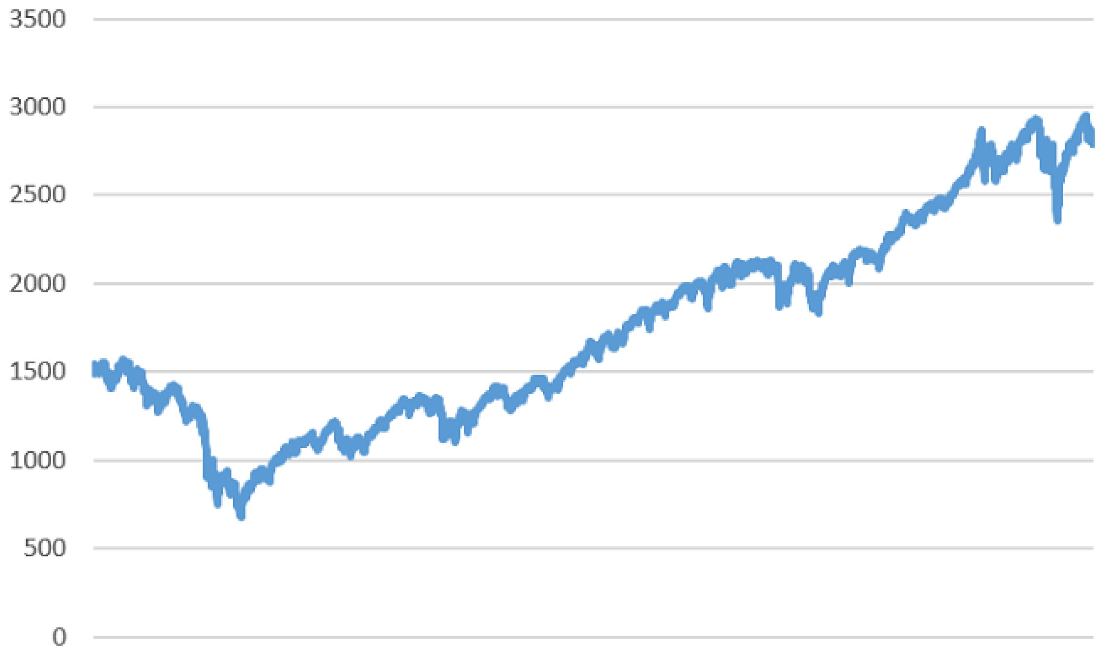
In order to evaluate the contribution of the smoothing techniques based on F-transform, we consider a time series of 3020 values (pictured in Figure 2), covering the time period form June 2007 to June 2019, of the S&P500 index which measures the cumulative float-adjusted market capitalization of 500 of the United States largest corporations.

The number n of subintervals in the fuzzy partition $(\mathbb{P},\mathbb{A})$ is $\frac{m}{16}.$ As in kernel smoothing, the basic functions $A_k\left(x\right)$, defined on the intervals $[x_{k-r},x_{k+r}]$, are obtained by translating and rescaling the same symmetric fuzzy number $A_0$, defined on $[-1,1]$ and centered at the origin, with membership

$$A_0\left(t\right)=\left\{\begin{array}{ccc}L(1+\tau ,{\beta }_0,{\beta }_1)\hfill & \mathrm{if}\hfill & \tau \in [-1,0]\hfill \\ 1-L(t,{\beta }_1,{\beta }_0)\hfill & \mathrm{if}\hfill & \tau \in [0,1]\hfill \\ 0\hfill & \hfill & \mathrm{otherwise}\hfill \end{array}\right.,$$

(13)

where the basic functions are increasing rational spline defined as

$$L\left(\tau \right)=\frac{{\tau }^2+{\beta }_0\tau (1-\tau )}{1+({\beta }_0+{\beta }_1-2)\tau (1-\tau )}\mathrm{for}\tau \in [0,1]$$

(14)

with slope parameters ${\beta }_0=0.5$, ${\beta }_1=0.5$. In general, the smoothing effect is not so much depending on the choice of function $A_0$, instead, the number n of subintervals of the decomposition P and the bandwidth r strongly impact the smoothing effect; the best combinations of n and r have been chosen by a generalized cross validation (GCV) approach.

Expectile and quantile smoothed curves $E_{\omega }\left(x\right)$ and $Q_{\omega }\left(x\right)$ (given a specific value $\omega \in [0,1]$) are obtained from the $\alpha$-cuts of the fuzzy-valued expectile function ${\widehat{f}}_{(\mathbb{P},\mathbb{A})}\left(x\right)$, as in (6) and the fuzzy-valued quantile function ${\tilde{f}}_{(\mathbb{P},\mathbb{A})}\left(x\right),$ as in (12) as follows:

$$E_{\omega }\left(x\right)=\left\{\begin{array}{ccc}{\displaystyle \sum _{k=1}^n}{F}_{k,2\omega }^{-}{A}_k\left(x\right)& \mathrm{if}& \omega \le \frac{1}{2}\\ {\displaystyle \sum _{k=1}^n}{F}_{k,2(1-\omega )}^{+}{A}_k\left(x\right)& \mathrm{if}& \omega \ge \frac{1}{2}\end{array}\right.$$

(15)

$$Q_{\omega }\left(x\right)=\left\{\begin{array}{ccc}{\displaystyle \sum _{k=1}^n}{G}_{k,2\omega }^{-}{A}_k\left(x\right)& \mathrm{if}& \omega \le \frac{1}{2}\\ {\displaystyle \sum _{k=1}^n}{G}_{k,2(1-\omega )}^{+}{A}_k\left(x\right)& \mathrm{if}& \omega \ge \frac{1}{2}.\end{array}\right.$$

(16)

As we mentioned in the introduction, historical simulation for Value at Risk estimation is the most widely implemented nonparametric approach but it is not always the best performing. Its main advantages can be phrased as follows—(1) generally the implementation is very easy, (2) it does not depend on parametric assumptions on returns distribution implying that it can accommodate wide tails, skewness and any other non-normal features in financial observations.

On the other hand, the strongest weakness is its completely dependence on the data set.

Many contributions find that historical simulation underestimates risk in an unusually quiet period and it is sometimes slow to reflect market turbulence. The non parametric smoothing methods based on F-transform can weaken these distortions as we show in some simple experiments.

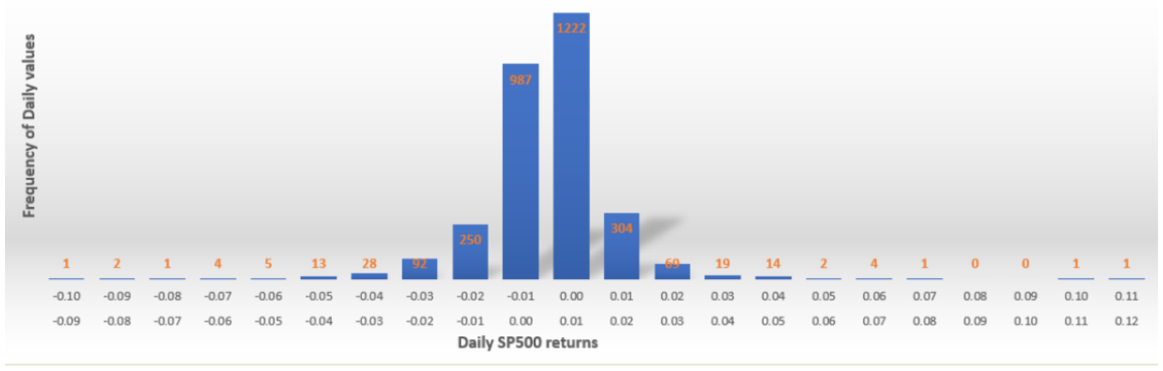
In our findings, when no smoothing technique is applied, the value VaR${}_{Hist}$ is computed for the time series of returns of S&P500 index which are plotted in Figure 3 and, as it is expected, show a quite modest volatility with a low numbers of values in the left tail. The 95% confidence level and the time period of one day imply that $Va{R}_{Hist}$ corresponds to the 5th quantile of the daily S&P500 returns with a negative sign because VaR is always interpreted as a loss.

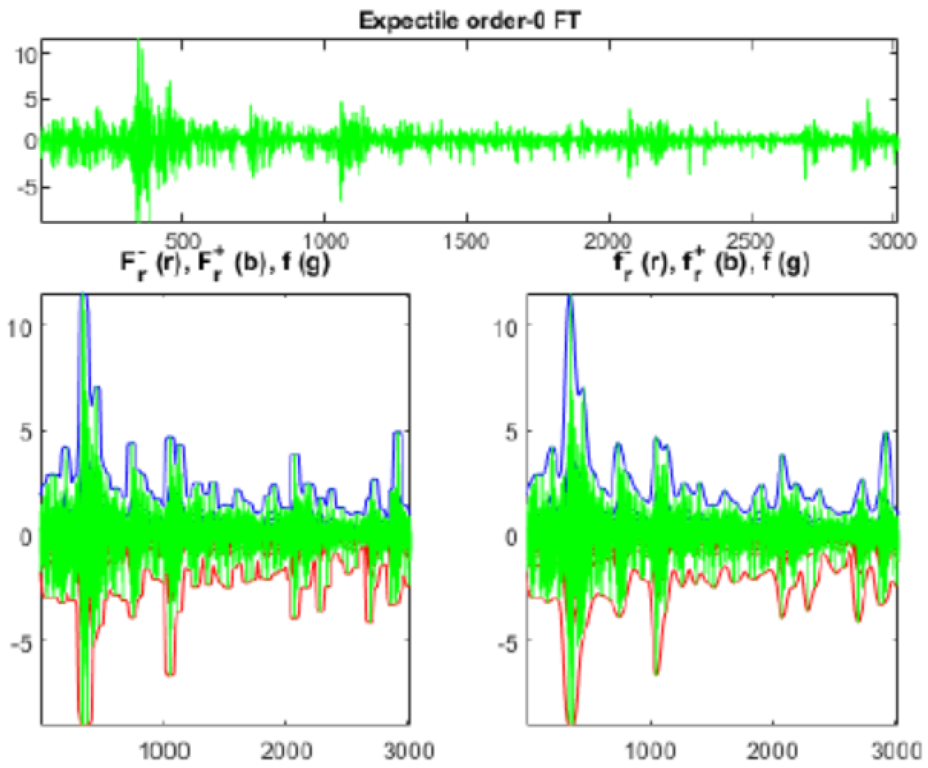
In Figure 4 the effects of the smoothing procedure based on $L_2-norm$ minimization (Figure 5 shows the dynamics of left and right minimizers) are applied for 3020 daily values of the S&P500 index, proving itself to be an efficient methodology.

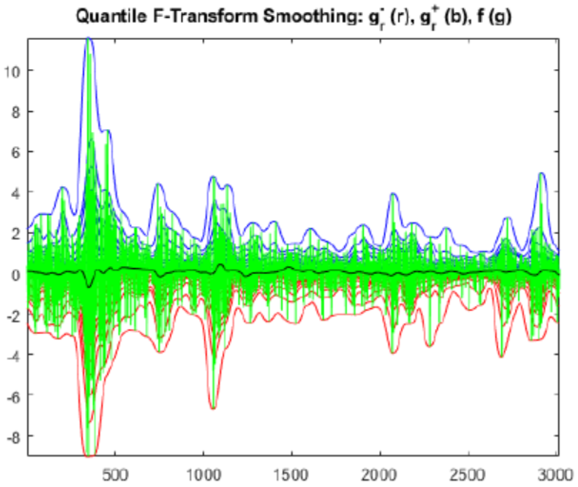
Figure 6 shows that the bandwidth of the quantile smoothing is slightly smaller than the expectile one, especially for the downside returns which mostly affect the Value at Risk; more evident differences could be appreciated in case of higher volatile time series.

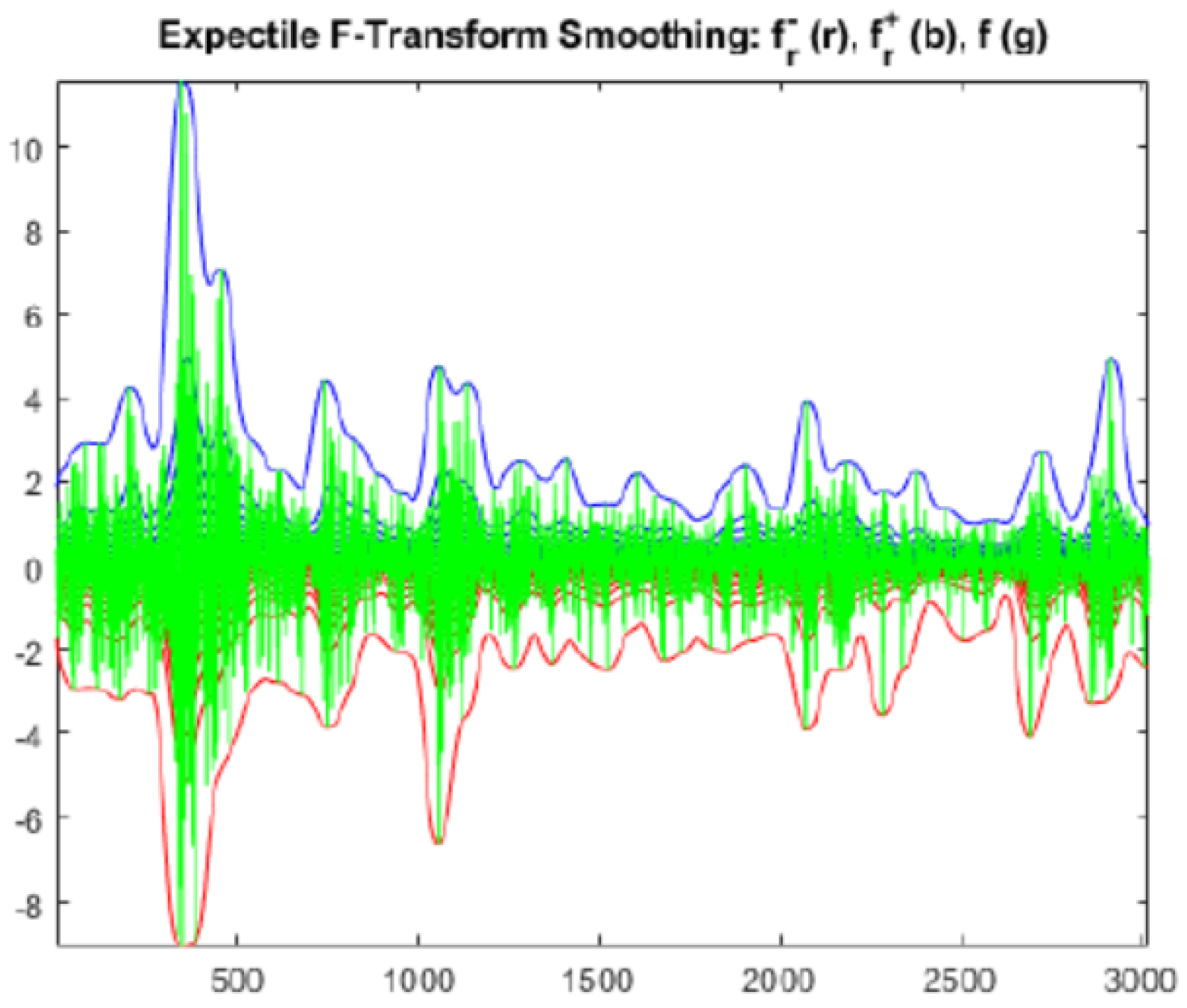
In Figure 7 the left and right minimizers in the smoothing procedure based on $L_1\text{-}norm$ minimization are represented.

Given the smoothed time series, VaR${}_{EXP}$ is the value obtained with the expectile smoothing, whereas VaR${}_{QUA}$ is the same value obtained with the quantile smoothing.

We consider rolling windows, each one made up of 500 observations (two financial years). S&P500 index returns within the first window are sorted in ascending order and the 5-quantile of interest is given by the return that leaves 5% of the observations on its left side and 95% on its right side. The 5% allows to include an higher number of returns, considering the small number of outliers. To compute the VaR the following day, the whole window is moved forward by one observation and the entire procedure is repeated.

Consequently, the first window consists of the returns from June 2007 to May 2009 for a total amount of 503 returns over a total of 3020. It implies that the first VaR is related to 1 June 2009 and the next values are related to each following day.

A back-testing procedure is adopted to compare the three VaRs in terms of violations which are the unpredicted losses with the actual losses realized on each day.

The back-testing analysis takes into account 2516 rolling windows for a total number of 2515 VaR values. The results are shown in

Table 1. Violations percentages.

95%	N	VaR${}_{\mathit{Hist}}$	VaR${}_{\mathit{EXP}}$	VaR${}_{\mathit{QUA}}$
2009	150	7.8%	7.2%	6.2%
2010	251	14.6%	13.76%	12.4%
2011	252	8.5%	7.1%	6.4%
2012	250	7.7%	7.2%	6.3%
2013	251	5.3%	5.1%	4.4%
2014	252	6.4%	5.9%	5.2%
2015	250	7.5%	7.1%	6.8%
2016	252	6.6%	6.6%	6.2%
2017	250	6.4%	6.3%	5.8%
2018	251	12.5%	11.3%	10.7%
2019	107	8.2%	7.7%	7.2%

which offers the possibility of some observations: first of all, the number of violations is slightly reduced when a smoothing methodology is applied and the reduction is more evident when the quantile one is performed, confirming its results extensively analyzed in [17].

4. Average Cumulative Function

The ACF-representation and its properties are studied in [20] where the relationship between ACF and quantile functions, which we apply to Value at Risk hereafter, is proved and resumed in what follows.

The ACF is a representation based on the following assumptions:

• u are real fuzzy intervals with compact support $[a,b]$ and compact nonempty core $[c,d]\subset [a,b]$ where $a\le c\le d\le b\in \mathbb{R}$, their space is ${\mathbb{R}}_{\mathcal{F}}$;
• the membership function of $u\in {\mathbb{R}}_{\mathcal{F}}$ can be represented in the form

  $$u\left(x\right)=\left\{\begin{array}{ccc}0& \mathrm{if}& x<a\\ u^L\left(x\right)& \mathrm{if}& a\le x<c\\ 1& \mathrm{if}& c\le x\le d\\ u^R\left(x\right)& \mathrm{if}& d<x\le b\\ 0& \mathrm{if}& x>b\end{array},\right.$$

  (17)

  where $u^L:[a,c]⟶[0,1]$ is a nondecreasing right-continuous function, $u^L\left(x\right)>0$ for $x\in [a,c]$, called the left side of the fuzzy interval and $u^R:[d,b]⟶[0,1]$ is a nonincreasing left-continuous function, $u^R\left(x\right)>0$ for $x\in [d,b]$, called the right side of the fuzzy interval. The two functions $u^L\left(x\right)$ and $u^R\left(x\right)$ are extended to the real domain by setting

  $$u_{ext}^L\left(x\right)=\left\{\begin{array}{ccc}0& if& x<a\\ u^L\left(x\right)& if& a\le x<c\\ 1& if& x\ge c\end{array}\right.$$

  (18)

  $$u_{ext}^R\left(x\right)=\left\{\begin{array}{ccc}1& if& x\le d\\ u^R\left(x\right)& if& d<x\le b\\ 0& if& x>b.\end{array}\right.$$

  (19)
• There exists a pair of cumulative distribution functions, called the lower cdf and the upper cdf of u, based on the extended left side function $u_{ext}^L\left(x\right)$ and the extended right side function $u_{ext}^R\left(x\right)$ such that $u\left(x\right)=F_u^L\left(x\right)-F_u^R\left(x\right)$ $\forall x\in \mathbb{R}$, where

  $$F_u^R\left(x\right)=1-u_{ext}^R\left(x\right)=\left\{\begin{array}{ccc}0& if& x\le d\\ 1-u^R\left(x\right)& if& d<x\le b\\ 1& if& x>b.\end{array}\right.$$

  (20)

  and

  $$F_u^L\left(x\right)=u_{ext}^L\left(x\right),$$

  (21)

implying that the $\lambda$-Average Cumulative function ($\lambda$-ACF) of u is defined for a fixed value of $\lambda \in [0,1]$ as the following convex combination of $F_u^L$ and $F_u^R$, for all $x\in \mathbb{R}$,

$$\begin{array}{ccc}{F}_u^{\left(\lambda \right)}\left(x\right)\hfill & =& (1-\lambda )F_u^L\left(x\right)+\lambda F_u^R\left(x\right)\hfill \\ \hfill & =& \left\{\begin{array}{ccc}0& \mathrm{if}& x<a\\ (1-\lambda )u^L\left(x\right)& \mathrm{if}& a\le x<c\\ 1-\lambda & \mathrm{if}& c\le x\le d\\ 1-\lambda u^R\left(x\right)& \mathrm{if}& d<x\le b\\ 1& \mathrm{if}& x>b,\end{array}\right.\hfill \end{array}$$

(22)

where $F_u^{\left(\lambda \right)}$ is non-decreasing, right continuous on $\left[-\infty ,d\right]$, left continuous on $\left[c,+\infty \right]$ and above all, its generalized inverse, defined by

$${\left(F_u^{\left(\lambda \right)}\right)}^{-1}\left(t\right)=inf\{x\in \mathbb{R}|F_u^{\left(\lambda \right)}\left(x\right)\ge t\}=sup\{x\in \mathbb{R}|F_u^{\left(\lambda \right)}\left(x\right)<t\}$$

(23)

is the quantile function of $F_u^{\left(\lambda \right)}$.

A quantile of order $p\in [0,1]$ for a cdf $F_X$ (or for the associated random variable X) is a real value ${\kappa }_p$ such that

$${\displaystyle \underset{x\uparrow {\kappa }_p}{lim}}{F}_X\left(x\right)\le p\mathrm{and}{F}_X\left({\kappa }_p\right)\ge p$$

(24)

and considering a simple sample $x_1,x_2,\dots ,x_N$ from a real random variable X; for a value of $p\in [0,1]$, the (empirical) p-quantile ${\widehat{\kappa }}_p\left(N\right)$ is obtained by minimizing, with respect to k, the following (empirical) function

$$S_{p,N}\left(k\right)=(1-p)\sum _{\begin{array}{c}i=1\\ x_i<k\end{array}}^N(k-x_i)+p\sum _{\begin{array}{c}i=1\\ x_i>k\end{array}}^N(x_i-k);$$

(25)

furthermore,

$${\widehat{\kappa }}_p\left(N\right)=arg\underset{k}{min}{S}_{p,N}\left(k\right)$$

(26)

is an unbiased estimate of ${\kappa }_p$.

A relevant property states that when the fuzzy intervals $u\in {\mathbb{R}}_{\mathcal{F}}$ have continuous membership function and $F_u\left(x\right)$, $x\in \mathbb{R}$ is their $\frac{1}{2}$-ACF, then for all $\alpha \in [0,1]$, the $\alpha$-cuts $[u_{\alpha }^{-},u_{\alpha }^{+}]$ of u are such that $u_{\alpha }^{-}$ is the $\frac{\alpha }{2}$-quantile of $F_u\left(x\right)$ and $u_{\alpha }^{+}$ is the $\frac{\alpha }{2}$-quantile of $F_{-u}\left(x\right)$.

In our financial experiments the fuzzy number $u\in {\mathbb{R}}_{\mathcal{F}}$ is “measured” at N (independent) observations $(t_i,u\left(t_i\right))$ which are the daily data of S&P500 index and this is equivalent to consider a set of independent variables $X_1,X_2,\dots ,X_N$ identically distributed on the support $\left[a,b\right]$ and to extract a simple sample of N distinct values $t_i$ from each $X_i$, $i=1,2,\dots ,N$.

Consider the decomposition ${\mathbb{P}}_N=\left\{x_1<x_2<\dots <x_N\right\}$ of the support $\left[a,b\right]$, obtained by ordering the $t_i$ such that $t_{\left(1\right)}<t_{\left(2\right)}\dots <t_{\left(N\right)}$ and defining $x_i=t_{\left(i\right)}$ for $i=1,2\dots ,N$. We define the corresponding empirical AC function as:

$${\widehat{F}}_{{\mathbb{P}}_N}\left(x\right)=\frac{1}{N}\sum _{i=1}^N\widehat{I}\left(x\ge x_i\right)$$

(27)

where

$$\widehat{I}\left(x\ge x_i\right)=\left\{\begin{array}{ccc}1& \mathrm{if}& x\ge x_i\\ 0& \mathrm{if}& x<x_i\end{array}\right..$$

(28)

For $\alpha \in ]0,1]$, the $\alpha$-cuts of u can be estimated by computing the empirical $\frac{\alpha }{2}$-quantile of the sample data $\left\{x_i\right|i:1,\dots ,N\}$ and the empirical $\frac{\alpha }{2}$-quantile of the data $\{-x_i|i:1,\dots ,N\}$. The two following empirical functions, as in Equation (25):

$$S_{\alpha }^{-}\left(m\right)=(1-\frac{\alpha }{2})\sum _{\begin{array}{c}i=1\\ x_i<m\end{array}}^N(m-x_i)+\frac{\alpha }{2}\sum _{\begin{array}{c}i=1\\ x_i>m\end{array}}^N(x_i-m)$$

(29)

and

$$S_{\alpha }^{+}\left(m\right)=\frac{\alpha }{2}\sum _{\begin{array}{c}i=1\\ x_i<m\end{array}}^N(m-x_i)+(1-\frac{\alpha }{2})\sum _{\begin{array}{c}i=1\\ x_i>m\end{array}}^N(x_i-m)$$

(30)

are minimized and the obtained values

$$\begin{array}{ccc}{m}_{\alpha }^{-}\left(N\right)\hfill & =& arg\underset{m}{min}{S}_{\alpha }^{-}\left(m\right)\hfill \end{array}$$

(31)

$$\begin{array}{ccc}{m}_{\alpha }^{+}\left(N\right)\hfill & =& arg\underset{m}{min}{S}_{\alpha }^{+}\left(m\right)\hfill \end{array}$$

(32)

give an estimate $[m_{\alpha }^{-}\left(N\right),m_{\alpha }^{+}\left(N\right)]$ of the $\alpha$-cut $[u_{\alpha }^{-},u_{\alpha }^{+}]$ of u and are obtained without computing directly the (empirical) AC function from the data; in addition, the estimated value $m_{\alpha }^{+}\left(N\right)$ is exactly the $(1-\frac{\alpha }{2})$-quantile of the sample data $\left\{x_i\right|i:1,\dots ,N\}$; so, the extreme values $u_{\alpha }^{-}$ and $u_{\alpha }^{+}$ of each $\alpha$-cut of u can be estimated, statistically, by an $\frac{\alpha }{2}$-quantile and an $(1-\frac{\alpha }{2})$-quantile, respectively.

5. Value at Risk Based on ACF

The ACF representation allows obtaining the guess quantiles directly from the time series because it has the same properties of a cumulative distribution function (CDF) of a (real) random variable X, defined on the same (support) domain.

Generally, the p-quantile of $F_{\alpha }\left(x\right)$ is the value

$$Va{R}_{ACF}=x_p=inf\left\{x|F_{\alpha }\left(x\right)\ge p\right\}=inf\left\{t:Pr\left(t\le x\right)\ge p\right\}$$

(33)

for any CDF of $F_{\alpha }\left(x\right)$ and for the given confidence level $p\in \left(0,1\right).$

Given the daily S&P500 index time series X, the quantile function (23) deduced from ACF allows the evaluation of $Va{R}_{ACF}\left[X;p\right]={\left(F_u^{\left(\lambda \right)}\right)}^{-1}\left(t\right),$ where in our experiments p is equal to $0.95$. Consequently, $VaR[X;0.95]$ gives the maximum risk, for the time horizon of one day, for the $100p\%=95\%$ of the cases.

The quantiles obtained through the ACF refine the recognition of the left side of the daily returns of S&P500 index in such a way that the forecasting capability is augmented and obviously the number of violations is strongly reduced. The percentage of violations for VaR${}_{ACF}$ (as shown in

Table 2. Percentages of violations.

95%	N	VaR${}_{\mathit{Hist}}$	VaR${}_{\mathit{ACF}}$
2009	150	7.8%	6.1%
2010	251	14.6%	10.3%
2011	252	8.5%	5.9%
2012	250	7.7%	6.1%
2013	251	5.3%	4.3%
2014	252	6.4%	5.3%
2015	250	7.5%	6.2%
2016	252	6.6%	5.5%
2017	250	6.4%	5.2%
2018	251	12.5%	8.6%
2019	107	8.2%	6.5%

) is considerably smaller in every year and the reduction becomes crucial in 2010 and 2018 when the high volatility in financial markets caused unsuitable capital allocations.

6. Closing Considerations

The adopted back-testing procedure studies the performance of the three values VaR${}_{EXP}$, VaR${}_{QUA},$ VaR${}_{ACF}$ in terms of the number of violations over 2515 values when they are compared to the value VaR${}_{Hist};$ violations have a strong concrete meaning because they detect all the days in which the actual losses are not predicted by the VaR estimation implying a scarce amount of capital for facing adverse situations.

Despite the limitation regarding the fact that only one single asset (S&P500 index) is tested, Table 1 and Table 2 show that VaR${}_{ACF}$ performing is effectively the best; in 2010 the percentage of violations moves from 14.6% for VaR${}_{Hist}$ to 10.3% for VaR${}_{ACF}$, also in 2018 the reduction has a similar order of magnitude. However, also the smoothing effects on returns are evident because the number of violations for VaR${}_{EXP}$ and VaR${}_{QUA}$ is reduced, even if in a more soft way. The limitation of a single asset can have a strong impact because an index is generally less volatile than a stock price, as it is computed as a weighted mean, and the smoothing effect could be theoretically mostly effective when the volatility is higher.

In VaR estimation through the ACF, the investigation of the properties which relate the non parametric estimation and the uncertainty modeling deserves a further appropriate theoretical investigation devoted to the combination between probability and possibility settings.

However, preliminary results strongly encourage the adoption of models based on Fuzzy set theory for calculating VaR and possibly several more risk measures, due to their capability to contemplate uncertainty in a rigorous way. The paradigm of uncertainty is crucial not only in financial time series but in the whole field of data science which includes all real life data, from social media to medicine, from ecology to history.

7. Paths for Future Research

The amount of promising research paths for uncertainty theories in risk management is huge (as described in [22]), here we just give a flavour of the most appealing from our point of view. Vagueness sources in real data can be viewed as a mixture of stochastic and fuzzy approaches as in [23] where a given interval describes the available information regarding the evolution of certain variables is vague. Also the possibility of introducing random-fuzzy variables (as in [24]) in the evaluation of risk measures deserves more efforts in order to be combined with the stochastic nature of the traditional model.

In order to extend the research from a unique stock to a portfolio, a possible research is to apply the introduced non parametric estimation in the case of a portfolio selection model with VaR constraint under different attitudes, as studied in [25].

A challenging future research path can be the extension of the proposed approaches within the field of neutrosophic logic (derived from the seminal philosophical paper by Samarandache in [26]) which is compared in [27] with well-known frameworks for reasoning with uncertainty and vagueness.

The concept of set highlights the main difference between fuzzy logic and neutrosophic logic; a fuzzy set is defined through association with a scale of grades of membership, its generalization is called intuitionistic fuzzy set and it assigns two values called membership degree and non-membership degree respectively, when an additional parameter for neutrality is introduced, then the neutrosophic fuzzy set is defined.

In particular, many contributions based on neutrosophic statistics (broadly detailed in [28]) are decisively successful when data have indeterminate observations. Consequently, classical statistical tests can be rephrased as in [29], where the Kolmogorov–Smirnov tests is applied when the data contain neutrosophic observations, or in [30], where a chi-square test of independence under indeterminacy is introduced; moreover, in [31] the Dixon’s test is extended within a complex systems when observations are not all determined as it happens in experiment’s results when testing the normality of the data through neutrosophic statistics as in [32]. In social sciences as Economics and Management the scarce availability of certain data can be approached through neutrosophic statistics as in [33], where an efficient and flexible acceptance criterion is introduced for a two-stage process for multiple lines. Also in medical science uncertainty is a common feature and neutrosophic statistics is a rigorous way to model it as it is shown in [34] where uncertain data from an healthcare department are analyzed and in [35] where an investigation is introduced to classify when patients have the diabetes or not.

In addition, widening the scenario of uncertainty modelling, the tail VaR metric on a tree network, as shown in [36], computes the probability of the loss and its severity in an uncertain environment.

Finally, the classical statistical research path in risk management is largely fertile; just to give an example, a recent nonparametric method (detailed in [37]) for VaR extracts the quantile of a conditional distribution which is estimated considering the density of the copula describing the dependence observed in the series of returns.

References

- Jorion, P. Value at Risk: The New Benchmark for Managing Financial Risk, 2nd ed.; McGraw-Hill: New York, NY, USA, 2001. [Google Scholar]
- Abad, P.; Benito, S.; López, C. A comprehensive review of Value at Risk methodologies. Span. Rev. Financ. Econ. 2014, 12, 15–32. [Google Scholar] [CrossRef]
- Shayya, R.; Terceño, A.; Sorrosal-Forradellas, M.T. Systematic Review of the Literature on Value-at-Risk Models. In Proceedings of the XX SIGEF Congress, Harnessing Complexity through Fuzzy Logic, Naples, Italy, 4–5 July 2019. [Google Scholar]
- Cherubini, U.; Della Lunga, G. Fuzzy value-at-risk: Accounting for market liquidity. Econ. Notes 2001, 30, 293–312. [Google Scholar] [CrossRef]
- Zmeskal, Z. Value at risk methodology under soft conditions approach (fuzzy-stochastic approach). Eur. J. Oper. Res. 2005, 161, 337–347. [Google Scholar] [CrossRef]
- Chen, W.S.; Gerlach, R.; Hwanga, B.K.; McAleer, M. Forecasting Value-at-Risk using nonlinear regression quantiles and the intra-day range. Int. J. Forecast. 2012, 28, 557–574. [Google Scholar] [CrossRef] [Green Version]
- Yoshida, Y. An estimation model of value-at-risk portfolio under uncertainty. Fuzzy Sets Syst. 2009, 160, 3250–3262. [Google Scholar] [CrossRef]
- Moussa, A.M.; Kamdem, J.S.; Terraza, M. Fuzzy value-at-risk and expected shortfall for portfolios with heavy-tailed returns. Econ. Model. 2014, 39, 247–256. [Google Scholar] [CrossRef]
- Almeida, R.J.; Kaymak, U. Probabilistic Fuzzy Systems in Value at Risk Estimation, Intelligent Systems in Accounting. Financ. Manag. 2009, 16, 49–70. [Google Scholar]
- Li, T.; Zhang, W.; Xu, W. Fuzzy possibilistic portfolio selection model with VaR constraint and risk-free investment. Econ. Model. 2013, 31, 12–17. [Google Scholar] [CrossRef]
- Maciel, L.; Ballini, R.; Gomide, F. An evolving possibilistic fuzzy modeling approach for Value-at-Risk estimation. Appl. Soft Comput. 2017, 60, 820–830. [Google Scholar] [CrossRef] [Green Version]
- Peña, A.; Bonet, I.; Lochmuller, C.; Patiño, H.A.; Chiclana, F.; Góngora, M. A fuzzy credibility model to estimate the Operational Value at Risk using internal and external data of risk events. Knowl.-Based Syst. 2018, 159, 98–109. [Google Scholar] [CrossRef] [Green Version]
- Peng, J. Credibilistic Value and Average Value at Risk in Fuzzy Risk Analysis. Fuzzy Inf. Eng. 2011, 1, 69–79. [Google Scholar] [CrossRef]
- Khraibani, H.; Nehme, B.; Strauss, O. Interval Estimation of Value-at-Risk Based on Nonparametric Models. Econometrics 2018, 6, 47. [Google Scholar] [CrossRef] [Green Version]
- Guerra, M.L.; Sorini, L.; Stefanini, L. Value function computation in fuzzy models by differential evolution. Int. J. Fuzzy Syst. 2017, 19, 1025–1031. [Google Scholar] [CrossRef]
- Kim, Y.; Lee, E. A Probabilistic Alternative Approach to Optimal Project Profitability Based on the Value-at-Risk. Sustainability 2018, 10, 747. [Google Scholar] [CrossRef] [Green Version]
- Guerra, M.L.; Sorini, L.; Stefanini, L. Quantile and Expectile Smoothing based on L1-norm and L2-norm F-transforms. Int. J. Approx. Reason. 2019, 107, 17–43. [Google Scholar] [CrossRef]
- Chen, J.M. On Exactitude in Financial Regulation: Value-at-Risk, Expected Shortfall, and Expectiles. Risks 2018, 6, 61. [Google Scholar] [CrossRef] [Green Version]
- Alemany, R.; Bolancé, C.; Guillén, M. A nonparametric approach to calculating value-at-risk. Insur. Math. Econ. 2013, 52, 255–262. [Google Scholar] [CrossRef]
- Stefanini, L.; Guerra, M.L. On possibilistic representations of fuzzy intervals. Inf. Sci. 2017, 405, 33–54. [Google Scholar] [CrossRef] [Green Version]
- Guerra, M.L.; Sorini, L.; Stefanini, L. On the approximation of a membership function by empirical quantile functions. Int. J. Approx. Reason. 2020, 124, 133–146. [Google Scholar] [CrossRef]
- Aven, T.; Baraldi, P.; Flage, R.; Zio, E. Uncertainty in Risk Assessment: The Representation and Treatment of Uncertainties by Probabilistic and Non-Probabilistic Methods, Engineering Statistics Series; Wiley: Hoboken, NJ, USA, 2014. [Google Scholar]
- Chen, Y.-C.; Chiu, Y.-H.; Huang, C.-W.; Tu, C.-H. The analysis of bank business performance and market risk-Applying Fuzzy DEA. Econ. Model. 2013, 32, 225–232. [Google Scholar] [CrossRef]
- Yoshida, Y. Maximization of Returns under an Average Value-at-Risk Constraint in Fuzzy Asset Management. Procedia Comput. Sci. 2017, 112, 11–20. [Google Scholar] [CrossRef]
- Zhou, X.; Wang, J.; Yang, X.; Lev, B.; Wang, S. Portfolio selection under different attitudes in fuzzy environment. Inf. Sci. 2018, 462, 278–289. [Google Scholar] [CrossRef]
- Smarandache, F. A Unifying Field in Logics: Neutrosophic Logic. Neutrosophy, Neutrosophic Set, Neutrosophic Probability; American Research Press: Rehoboth, NM, USA, 1999. [Google Scholar]
- Rivieccio, U. Neutrosophic logics: Prospects and Problems. Fuzzy Sets Syst. 2008, 159, 1860–1868. [Google Scholar] [CrossRef]
- Smarandache, F. Introduction to Neutrosophic Statistics; Infinite Study: Columbus, OH, USA, 2014. [Google Scholar]
- Aslam, M. Introducing Kolmogorov—Smirnov Tests under Uncertainty: An Application to Radioactive Data. ACS Omega 2020, 5, 914–917. [Google Scholar] [CrossRef] [PubMed] [Green Version]
- Aslam, M.; Arif, O.H. Test of Association in the Presence of Complex Environment. Complexity 2020. [Google Scholar] [CrossRef]
- Aslam, M. On detecting outliers in complex data using Dixon’s test under neutrosophic statistics. J. King Saud Univ. Sci. 2020, 32, 2005–2008. [Google Scholar] [CrossRef]
- Albassam, M.; Khan, N.; Aslam, M. The W/S Test for Data Having Neutrosophic Numbers: An Application to USA Village Population. Complexity 2020. [Google Scholar] [CrossRef]
- Aslam, M.; Raza, M.A.; Ahmad, L. Acceptance Sampling Plans for Two-Stage Process for Multiple Manufacturing Lines under Neutrosophic Statistics. J. Intell. Fuzzy Syst. 2019, 36, 7839–7850. [Google Scholar] [CrossRef]
- Aslam, M.; Arif, O.H. Multivariate Analysis under Indeterminacy: An Application to Chemical Content Data. J. Anal. Methods Chem. 2020, 6, 1406028. [Google Scholar]
- Aslam, M.; Arif, O.H.; Sherwani, R.A.K. New Diagnosis Test under the Neutrosophic Statistics: An Application to Diabetic Patients. BioMed Res. Int. 2020. [Google Scholar] [CrossRef] [Green Version]
- Soltanpour, A.; Baroughi, F.; Alizadeh, B. The inverse 1-median location problem on uncertain tree networks with tail value at risk criterion. Inf. Sci. 2020, 506, 383–394. [Google Scholar] [CrossRef]
- Geenens, G.R. A nonparametric copula approach to conditional Value-at-Risk. Econ. Stat. 2020. [Google Scholar] [CrossRef]
Figure 1.
Cumulative number of articles published on models for Value at Risk.
Figure 2.
Daily values of the S&P500 index within the period from June 2007 to June 2019.
Figure 3.
Distribution of S&P500 returns from June 2007 to June 2019.
Figure 4.
Effects of the expectile smoothing on a twelve years time series of daily returns of the S&P500 index.
Figure 5.
Graphical representation of the minimizers in Equation (2) when developing expectile smoothing.
Figure 6.
Quantile smoothing for twelve years of daily S&P500 index returns.
Figure 7.
Minimizers of Equation (8) in quantile smoothing.