Deep Reinforcement Learning Agent for S&P 500 Stock Selection

Abstract

This study investigated the performance of a trading agent based on a convolutional neural network model in portfolio management. The results showed that with real-world data the agent could produce relevant trading results, while the agent’s behavior corresponded to that of a high-risk taker. The data used were wide in comparison with earlier reported research and was based on the full set of the S&P 500 stock data for twenty-one years supplemented with selected financial ratios. The results presented are new in terms of the size of the data set used and with regards to the model used. The results provide direction and offer insight into how deep learning methods may be used in constructing automatic trading systems.

1. Introduction

Efficient and profitable portfolio management is one of the key functions of the financial industry and is on the top of the list of things that investors are looking for when making investments. This study was based on previous observation of modern portfolio theory developed by Markowitz [1], which is based on using historical returns, which may not, after all, be a fully efficient way to make portfolio selections (see e.g., [2,3]) or at least there exist complements to the selection process that offer new insights [3]. These new insights may be in the form of finding alternative ways to uncover abnormal returns with active asset allocation and stock selection [2,4,5]. Market anomalies are discrepancies between what is taking place in real-world markets and the theory of efficient markets. If market anomalies can be identified before they disappear, they can typically be turned into excess returns. Therefore, within the context of profitable portfolio management, the constant search for and the ability to utilize new market anomalies is of the essence. In this paper, we attempted to use an automated deep reinforcement learning based trading agent to create and put into action an arbitrage trading scheme in the context of historical S&P 500 data. Some of the more widely cited studies on market anomalies include Titman and Jegadeesh [6] on the existence of “momentum”, Banz [7] on “small-capitalization firms”, Basu [8] on the “earnings-to-price ratio” (E/P), and Fama and French [9] on “dividend yields”. It has been observed that reported market anomalies tend to vanish after they are made public [10].

The previous literature has already shown that classical mean-variance optimization of portfolios leads to poor results. In vein with the above, the key idea of this research is to concentrate on how portfolio management can be aided by the use of modern business analytics, namely, by using an artificial neural network (ANN)-based system to automatically detect market anomalies by technical analysis and to exploit them to maximize portfolio returns by realizing excess returns. An artificial neural network is a tool that is based on machine learning (ML), which is a field of scientific study that focuses on algorithms that learn from data. Machine learning has become popular also in the context of applied and mathematical finance, where credit scoring [11] and credit card fraud detection [12] are good examples of real-world use of ML-based systems from outside of portfolio management. Machine-learning based trading and trading systems have previously been studied in a number of works, (e.g., [13,14,15,16]).

Previous academic literature on portfolio management with specifically ANN-based systems [17,18,19,20] have shown promising results, but the reported research has so far used relatively small data sets and the focus has primarily been on comparatively demonstrating the abilities of different system and/or algorithm architectures. Kim and Kim [21] studied index tracking by creating a tracking portfolio (with S&P 500 stocks) with deep latent representation learning, and Lee and Kang [22] tried to predict the S&P 500 Index with an ANN.

In this study, we used the Ensemble of Identical Independent Evaluators (EIIE) architecture proposed by Jiang, Xu, and Liang [19] and apply it to a sample of 415 stocks (a larger sample than ever previously used) from the S&P 500 Index and, as a novelty, included selected performance indicators for stock performance in the analysis. For this research, we constructed an ANN-based deep-learning (multi-layer ANN) agent model for portfolio management (trading model) that was based on reinforcement learning. The agent model was guided by a reward function and the goal was to maximize the expected rewards over time. For a technical introduction to reinforcement learning and artificial neural networks, we refer the reader to [23].

A Short Literature Review of Using Reinforcement Learning Based Methods

Several studies have suggested that reinforcement learning methods can be used to tackle problems identified by the use of traditional optimization methods in portfolio management. Moody and others [24] used recurrent reinforcement learning for asset allocation to maximize risk-adjusted returns for a portfolio. They applied a differential Sharpe ratio as the reward function, and their method was found to outperform methods based on running- and moving-average Sharpe ratios in out-of-sample performance. Optimization of a differential Sharpe ratio was possible with a policy gradient algorithm thus being computationally less expensive while also enabling online optimization.

Moody and Saffel [17] studied a direct policy optimization method that used a differential downside ratio to better separate the undesirable downside risk from the preferred upside risk. The optimization method used in their research, referred to as “direct reinforcement”, has provided to be the basis for further studies [25,26]. Lu [25] tackled the portfolio optimization problem with direct reinforcement and used a policy gradient algorithm to maximize the differential Sharpe ratio and downside-deviation ratios with long short-term memory (LSTM) neural networks to implement forex trading. Almahdi and Yang [26] extended the use of direct reinforcement to a five-asset allocation problem and used the Calmar ratio as the to-be-optimized performance function of an exchange-traded fund (ETF) portfolio.

Lee and others [18] used a multi-agent approach with a cooperative Q-learning agent framework to carry out stock selection that consisted of two signal agents and two order agents that were in charge of executing the buy and sell actions. The system was able to efficiently exploit the historical intraday price information in stock selection and order executions. Ding and others [27] used deep convolutional networks to extract events from financial news to predict the long- and short-term movements of the S&P 500 Index.

Jiang, Xu, and Liang [19] successfully applied deep reinforcement learning to crypto-currency portfolio management. In their work, they proposed the “Ensemble of Identical Independent Evaluators” method. This method uses shared parameters that allow scalability to large data sets without a significant effect on computational requirements; this is an advantage over several other methods. Their method was later applied by Liang and others [20] to Chinese stock market data with improvements to the method; they achieved improved results with a small data set. Aboussalah and Lee [28] tested real-time portfolio optimization using the Sharpe ratio as the performance metric with a stacked deep dynamic recurrent reinforcement learning with an hour-glass-shaped network. They used ten stocks from the S&P500.

While the previous literature suggests that deep reinforcement learning has the potential as a tool for portfolio management, a recent paper by Liang and others [20] showed that the performance of studied deep reinforcement learning models was significantly lower than what was reported in previous studies. This suggests that the use of reinforcement learning and other machine learning models in stock trading and portfolio management has possibly already found its way to the practice of trading, and the anomalies exploited by their use disappear very fast and leave very little room for extraordinary returns.

With respect to the existing literature, the contribution of this paper is two-fold, first, the results of this research show that reinforcement learning-based methods, backed up with stock performance indicator data, are a relevant option for large-scale portfolio optimization. This extends the scientific knowledge from the great majority of the previous works, where only small portfolios were built from a limited set of available stocks that were optimized and constructed. Second, the agent developed in the study was proven to improve the performance of the stock portfolio in a way that is statistically significant, and its self-generated trading policy led to an impressive 328.9% return over the five-year test period. These findings are new and relevant both academically and for practitioners.

This paper is organized as follows: The following sections introduces the theoretical background, the data used, and then the model used for the trading agent and the environment are explained. Next, the feature and hyper-parameter selection and model training are presented, and the obtained results and the analyses of the model’s behavior are provided. The final section draws the findings together and describes some ideas for future research.

2. Theoretical Background

This section briefly describes the central methods underlying this research including convolutional neural networks, recurrent neural networks, reinforcement learning, and Markov decision processes.

Artificial neural networks (ANNs) are inspired by physical neural systems and are composed of interconnected neurons. A convolutional neural network (CNN) is an artificial neural network with a specific type of network architecture that combines information with a mathematical operation called convolution. The architecture is based on allowing parts of the network to focus on parts of the data (typically a picture) and the detection of the “whole picture” is a combination of the parts using convolution. Convolutional neural networks have been found to work well with pattern recognition and, consequently, they are primarily used to detect patterns from images. Krizhevsky and others [29] released a system called ImageNet, based on CNNs that revolutionized image classification. ImageNet contains five convolutional layers and millions of parameters, where the features in the lower-level layers capture primitive shapes, such as lines, while the higher-level layers integrate them to detect more complex patterns [23]. This allows ImageNet to detect highly complex features from raw pixels and separate them into different classes. Convolutional layers can be stacked on top of each other to detect more complex patterns from the data. Convolutional neural networks also have applications in areas such as natural language processing [30], and they have also been used in recognizing patterns from financial time series data [19].

Recurrent neural networks (RNNs) are a class of artificial neural networks designed to model sequential data structures like text sentences and time series data [23]. The idea behind recurrent networks is that the sequent observations are dependent on each other and, thus, the following value in a series depends on (several) previous observations. Sequential data are being fed to the network, and, for every observation, the network generates an output and an initial state that affects the next output. Recurrent neural networks have been used effectively, for example, in speech recognition [31] as well as in time series prediction [32].

In reinforcement learning (RL), the process of learning happens through trial and error without pre-existing information about behavior that leads to the maximization of a reward function [33] (1-2). Complex Markov decision processes (MDPs) can be optimized with different reinforcement learning algorithms that exploit function approximation, in which case the full model of the “environment” surrounding the problem is not necessary. Deep reinforcement learning (DRL) exploits ANNs in function approximation, and it has already been successfully applied to several areas such as robotics, video games [34,35,36], and finance [19,20]. Recent studies by Liang et al. [20] also showed some preliminary evidence about the ability of reinforcement learning models to learn useful factors from market data that can be used in portfolio management.

Sutton and Barto (p. 47) [33] define the MDP as a classical formalization of decision making, where performed actions influence, in addition to immediately reward, subsequent states, and through them future provide rewards. A Markov decision process consists of a set of different states, between which one can “travel” by taking action from a specific set of actions. By resolving the optimal action for all possible states, the optimal solution for a whole problem (a combination of actions to take), the optimal policy, can be reached [37]. The optimal behavior can be derived simply by estimating the optimal value function, v∗, for existing states with the Bellman equation. A policy which satisfies the Bellman optimality equation, v∗(s), (Equation (1)) is considered an optimal policy [33], p. 73).

$$v_{*}\left(s\right)=\underset{a}{\max }\mathbb{E}\left[R_{t+1}+\gamma v_{*}\left(S_{t+1}\right) | S_t=s, A_t=a\right]=\underset{a}{\max }{\displaystyle \sum }_{s^{\prime },r}p\left(s^{\prime },r|s,a\right)\left[r+\gamma v_{*}\left(s^{\prime }\right)\right],$$

(1)

where s represents the current state, s’ represents the following state, and a represents the action in the current state.

3. Data

The data used consisted of observations for 5283 days for 415 stocks that constitute the S&P 500 stock market index and covered a period of twenty-one years from 1998 to the end of the year 2018. Eighty-five stocks were discarded from the original 500 due the fact of observed problems with the quality of the data available. The data were mainly collected from Thomson Reuters Datastream and supplemented with figures available from Nasdaq.com in the case of missing data points.

The data used contained values for the total return index, closing prices, trading volumes, quarterly earnings per share, the out-paid dividends, and the declaration dates for dividends as well as the publication dates for the quarterly reports. The total return index was used to calculate the daily total return (TR) for each stock. The daily closing prices, quarterly earnings per share, and the publication dates for the quarterly reports were used to form a daily EP (EP) ratio for each stock that represented the stock’s profitability based on the latest reports. The quarterly dividends with the daily closing prices and the declaration dates were used to construct the daily dividend yield (DY) for each stock. The S&P 500 constituents were selected due to the fact of their high liquidity in the markets. High liquidity stocks suffer less from price slippage, and their price fluctuations are typically not caused by individual trades. This choice was made to ensure that the used model cannot exploit unprofitable patterns that might appear with less traded stocks due to the fact of low liquidity. The data set was remarkably larger than the data sets used in previous studies and, as such, served also as a test of the scalability of the (technology behind the) trader agent and allowed the discovery of whether a larger amount of stocks (data) positively affected the model performance. The three performance indicators for stocks—earnings to price, dividend yield, and trading volume—were selected as extra information to complement the information contained within the daily prices. The choice was made based on previous findings by [5,8,9] on the usefulness of these specific indicators in stock return prediction.

The data set was split into training, validation, and test sets such that the training data covered 14 years in total from 1998 to the end of 2011, the validation set two years from 2012 to 2013, and the test set five years from 2014 to 2018. The training data were used for training the agent system, while its performance was evaluated with the validation data. Test data were data that the agent system “has not seen before”, and it was used to test the performance of the trained model. It should be noted that the data set must be split in chronological in order to produce reliable results, since (in real-life) actual trading takes place with data that are new to the system. Splitting the data into training, validation, and test sets in a non-chronological order likely creates a look-ahead bias and may lead to unrealistic results. This is different to most typical algorithm tuning, where the data sets can be randomly split into training, validation, and test sets.

4. The Trading Environment and Agent Model Used

The real-world stock-market environment in which the agent model operated was modeled as an MDP. The MDP was defined with a four-tuple (S, A, P, R), where S is the set of states, A is the set of actions, P is the transition probability between the states, and R is the reward for action A in the state S. State S corresponds to the currently available market information and is represented with the input tensor $s_t$, which is a tensor of rank 3 with shape (d, n, f), where d is a fixed amount defining the length of the observation in days, n is the number of stocks in the environment, and f is the number of features for an individual stock.

The agent interacts with the environment by receiving the rank 3 tensor $s_t$ that represents the market state S and by outputting action A which is represented by the action-vector $a_t=\pi \left(s_t\right)$, where π is the current policy. In other words, the agent is “fed” $s_t$, based on which it outputs A that leads to reward R with the probability P. Market-state tensor takes shape based on fifteen observation days, 415 stocks, and the three features (TR, EP, DY). The action-vector equals in length the amount of 415 stocks and defines the (new) portfolio weights for the full set of stocks so that ${\displaystyle \sum }_{i=0}^n{a}_{i,t}=1$. The trader-agent picks and manages a 20 stock portfolio with a cash asset among the 415 stocks and is trained to maximize the Sharpe ratio for the portfolio. The effect of picking a 20 stock portfolio is constructed by setting all the portfolio weights other than the 20 largest weights to zero. The next-day portfolio return, following the action $a_t$, is constructed with the dot product $a_t·y_t$, where $y_t$ is the stock return vector.

Transition probability $P$ is the probability that the action $a_t$ at state $s_t$ leads to the state $s_{t+1}$. The transition probability function remains unknown for the portfolio management problem, and a model-free solution is used since market data are very noisy and the environment is too complex and only partially observable. The reward $R$ is defined with a future Sharpe ratio for a time interval $\left[t,t+T\right]$. Motivated by [24], a differential Sharpe ratio was used as the reward function, which was constructed in this study using Equation (2):

$$J_{\left[t,t+T\right]}\left({\pi }_{\theta }\right)=R\left(s_t,{\pi }_{\theta }\left(s_t\right),\dots ,s_{t+T},{\pi }_{\theta }\left(s_{t+T}\right)\right)=\frac{250}{T*\sqrt{250}*{\sigma }_{\left[t,t+T\right]}}{\displaystyle \sum }_t^{t+T}{a}_t·y_t$$

(2)

where the term $J_{\left[t,t+T\right]}\left({\pi }_{\theta }\right)$ represents an expected finite-horizon reward for the period $\left[t,t+T\right]$, when following the policy $\pi$, with parameters $\theta$. It is derived from the reward $R$, achieved from the state–action pairs during the period. A differential Sharpe ratio is represented as a mean of the daily portfolio returns $a_t·y_t$ divided by the standard deviation ${\sigma }_{\left[t,t+T\right]}$ of the portfolio during the time interval $\left[t,t+T\right]$.

The policy gradient algorithm was selected to optimize the differential Sharpe ratio for the model based on the good performances observed in several previous studies [19,20,24]. The policy gradient methods were found to outperform value-based methods with very noisy market data. The optimal policy ${\pi }^{*}$ is achieved when the expected reward $J\left({\pi }_{\theta }\right)$ is maximized, which is done by computing the gradient of the expected reward with respect to the policy parameters ${\nabla }_{\theta }J\left({\pi }_{\theta }\right)$ and by updating the policy parameters until the algorithm stops converging with Equation (3):

$${\theta }_{k+1}={\theta }_k+\alpha {\nabla }_{\theta }J\left({\pi }_{{\theta }_k}\right)$$

(3)

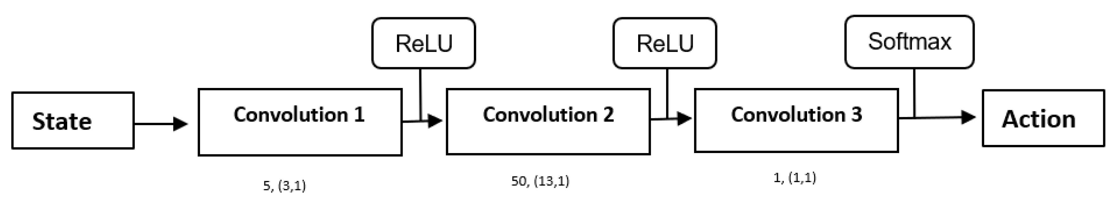
where $\alpha$ is the learning rate. The ANN agent model consists of three convolutional layers and is significantly inspired by the EIIE-method [19]. The structure used fits well for large-scale market data analysis due to the scalability permitted by the shared parameters. The first network layer includes small filters for extracting very basic level patterns from the data. The second network layer contains filters for matching shapes (exactly) with the first layer feature maps and produce feature maps of shape (1). The third network layer combines the feature maps as scalars to a vector of length n_stocks, which is placed into a softmax activation function to define the weight for each stock. Softmax is used for the final layer to produce a vector, which has a sum of 1 so that the most attractive stock gets the highest weight and all the wealth is always fully invested in assets. The basic structure of the model is represented in Figure 1.

The agent executes daily actions that determine the portfolio weights for the next day, to maximize the future risk-adjusted returns. This arrangement suggests that the stock portfolio can always be constructed with an exact set of weights. This is a simplification that is not fully realistic, since the prices of stocks vary considerably and prevent the construction of exactly weighted portfolios. In our model, this means that the agent can buy fractions of stocks to achieve precise weights. Transaction costs are taken into consideration as a daily fee that reduces the daily return.

Transaction costs are defined based on the commissions used by the Interactive Brokers 2019 prices, which is a popular broker for active trading. A fixed commission fee of 0.005 USD per a single traded stock is paid. On average the price of a stock in the data set was 60 USD, so $\frac{0.005}{60}{\displaystyle \sum }_{i=0}^n\left|w_{i,t}-a_{i,t}\right|$ a transaction cost was charged after each trade, where $w_t$ is the current portfolio weight vector. Due to the price movements affecting the portfolio weights, the portfolio weight vector $w_t$ was derived from the action vector $a_{t-1}$ by Equation (4):

$$w_t=\frac{a_{t-1}\times y_{t-1}}{a_{t-1}·y_{t-1}}$$

(4)

where $y_{t-1}$ is the stock return vector at time $t-1$. The simplification of the transaction costs does not, to the best of our understanding, cause a significant error in the analysis.

The Python programming language was used to construct the models using the TensorFlow^® library.

5. Training, Validation, and Results

This section presents the feature selection made to find the best-functioning model, the hyper-parameter selection with selection-supporting test results, the training and testing phases of the model with results, and an analysis of the model behavior.

5.1. Feature and Hyper-Parameter Selection

The first step in defining the final model used in the trading agent was to test the performance effect of four different combinations of features in three selected ANN model architectures. This means the testing of four different combinations of the financial ratios, already described above and including the total return index (TR), trading volume (Vol), dividend yield (DY), and daily earnings ratio (EP) for the stocks. The idea is to use TR and to include features that improve performance over TR alone; this is why the combinations tested were TR alone, TR and EP, TR and DY, and TR and Vol.

All of the three tested ANN model architectures included three layers, where the number of nodes in the first and the second layer was different for the three feature selection models, while the third layer used was identical. The models used in feature selection are designated A, B, and C, and the details of their layer-by-layer structure (i.e., number of filters) and the hyper-parameter values (i.e., shape of filters) used in the feature selection are visible in

Table 1. Feature selection results with the validation data set. Sharpe ratio and total return for the three models, with four feature-combinations. Legend: TR = Total Return; EP = Earnings Per Share; DY = Divided Yield; Vol = Volume

	Model	Layer 1	Layer 2	Layer 3	TR	TR, EP	TR, DY	TR, Vol
Sharpe	A	2, (2,1)	20, (14,1)	1, (1,1)	1.99	2.03	2.06	1.95
	B	3, (2,1)	50, (14,1)	1, (1,1)	2.18	2.18	2.27	1.94
	C	5, (2,1)	100, (14,1)	1, (1,1)	2.20	2.25	2.22	2.07
Total Return	A	2, (2,1)	20, (14,1)	1, (1,1)	86.38%	88.76%	72.08%	66.73%
	B	3, (2,1)	50, (14,1)	1, (1,1)	82.42%	82.11%	80.14%	68.87%
	C	5, (2,1)	100, (14,1)	1, (1,1)	87.23%	114.14%	88.02%	74.46%

. We acknowledge that the choice of using only three model architectures limits the reliability of the results; however, we feel that for the purposes of this research (to determine whether a feature contributes or not to the performance) it is sufficient.

The agent model was trained using mini-batches (b = 50, d = 15, n = 20, f = 1…4), where b is the batch length, d is the length of observation days, n is the amount of randomly selected stocks to the single batch, and f is the number of features used to train the model. The training was done in epochs of 500 mini-batches, and after each epoch, the model performance was evaluated with the validation data. To improve the model’s performance, normally distributed noise, with a standard deviation of 0.001 was added to the training data before feeding each batch to the model; this was in the same vein as Liang et al. (2018).

The feature selection model C had the most complex structure of the three models tested. It had the best performance in all cases measured in total return and in two out of three cases measured with the Sharpe ratio. The model B was best when measured with the Sharpe ratio and with the feature set TR and DY. Model A was the least complex (lowest number of filters) and had a performance that was inferior to model C across the board, while it outperformed model B and measured with total returns with two combinations. We note that [19] used a model structure that corresponds in complexity to that of Model A in their research on cryptocurrency trading. Table 1 shows the results received from the three feature selection models obtained with the validation data set.

The highest performance in terms of Sharpe ratio was achieved using TR and DY, but also the combination TR and EP improved the model’s performance slightly compared to using only TR. The results indicate that the combination of TR and Vol returned lower performances than TR alone. Based on the results, the features EP and DY were selected to be included in addition to TR in the final model.

Hyper-Parameter Selection

Hyper-parameter selection in this context means choosing the number of convolutional layers, the number of filters, and the shape of the filters used. To find a set of good hyper-parameters for a final model, ten initial “hyper-parameter selection models” with different hyper-parameter combinations were created based on the feature selection results and the fact that the most complex model (model C) used outperformed the simpler models. This means that the hyper-parameters for the ten initial models were selected semi-randomly using a higher complexity model structure as a starting point. The performance results for the initial ten models are visible in

Table 2. Performance of the ten initial and five-second-round hyper-parameter selection models. Model parameters given as number of filters, (filter shape). Model 14 (highlighted) had the best performance and was selected to be the final model version.

	Layer 1	Layer 2	Layer 3	Layer 4	Sharpe	Total Return
Model 1	3, (2,1)	50, (14,1)	1, (1,1)	-	2.15	80.85%
Model 2	4, (2,1)	100, (14,1)	1, (1,1)	-	2.34	99.07%
Model 3	3, (3,1)	50, (13,1)	1, (1,1)	-	2.25	105.44%
Model 4	5, (2,1)	100, (14,1)	1, (1,1)	-	2.21	79.83%
Model 5	5, (3,1)	70, (13,1)	1, (1,1)	-	2.11	115.84%
Model 6	10, (2,1)	100, (14,1)	1, (1,1)	-	2.40	104.73%
Model 7	20, (2,1)	200, (14,1)	1, (1,1)	-	2.26	88.84%
Model 8	3, (1,1)	3, (2,1)	50, (14,1)	1, (1,1)	2.15	84.02%
Model 9	3, (1,1)	4, (2,1)	100, (14,1)	1, (1,1)	2.14	69.54%
Model 10	3, (2,1)	5, (2,1)	100, (13,1)	1, (1,1)	2.19	88.62%
Model 11	8, (2,1)	80, (14,1)	1, (1,1)	-	2.24	101.04%
Model 12	8, (3,1)	80, (13,1)	1, (1,1)	-	2.25	83.89%
Model 13	5, (3,1)	100, (13,1)	1, (1,1)	-	2.32	99.23%
Model 14	5, (3,1)	50, (13,1)	1, (1,1)	-	2.43	118.06%
Model 15	10, (3,1)	100, (13,1)	1, (1,1)	-	2.26	79.95%

and indicated as models 1 through 10. Model 6 achieved the best validation performance in terms of the Sharpe ratio (2.40), while Model 5 achieved the highest total return (115.84%).

After the results from testing the ten initial hyper-parameter selection models, another five models were created based on the hyper-parameters from the best two initial round models. These five models are nominated models 11 through 15, and their hyper-parameter details and test results are visible in Table 2. Of the five second-round models, model 14 had the best performance measured with both metrics. Based on this two-tier hyper-parameter selection, model 14’s architecture was chosen as the final model architecture to be used in the trading agent.

The different models were trained for 300 epochs each. The results are presented as maximum 10 day rolling average Sharpe ratios and total returns. The rolling average was used to account for the possible problems with the unbalanced performance that may return extremely good “outlier” results that would nevertheless be non-representative of average model performance.

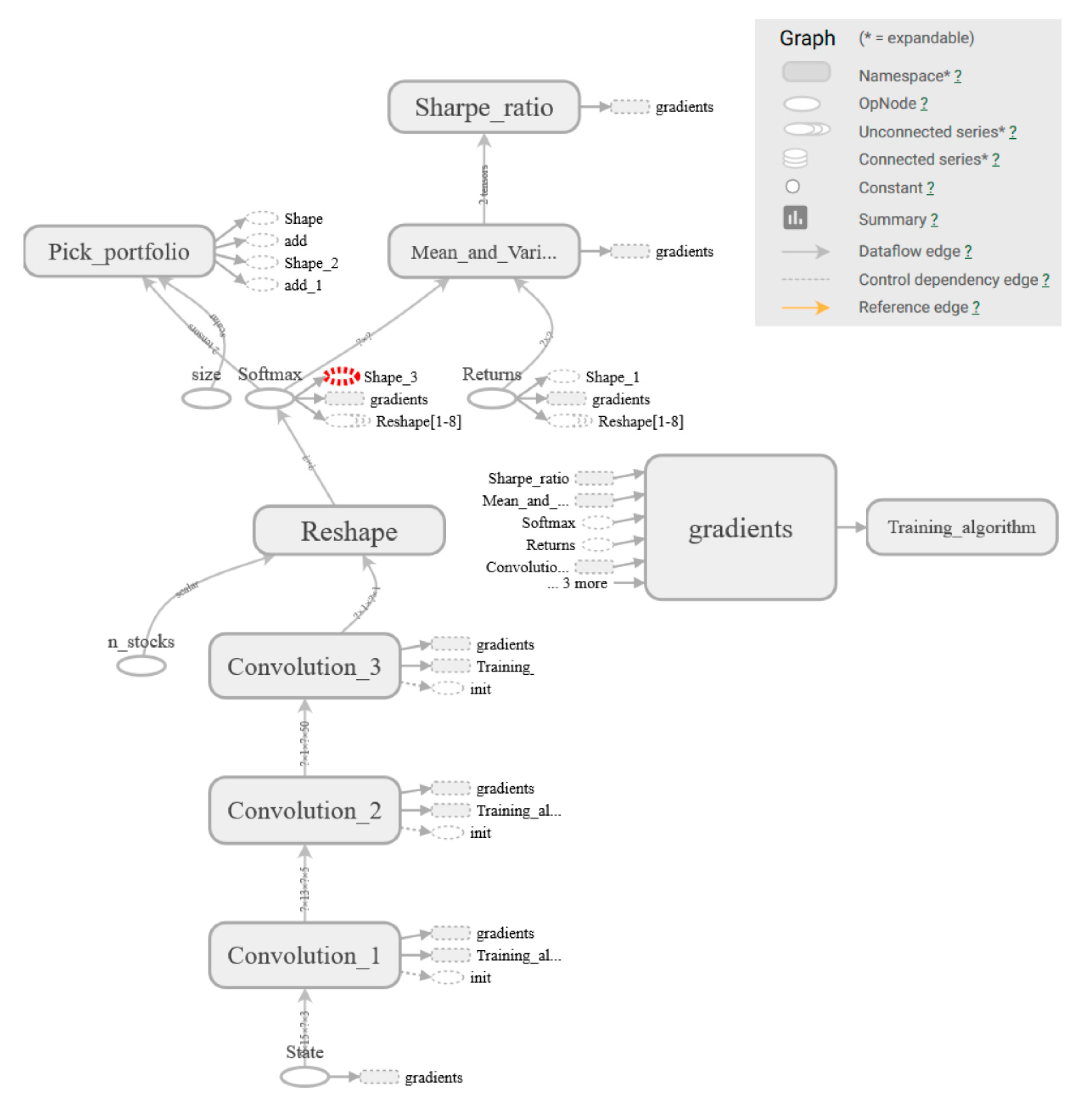
All models tested learned useful factors from the pure daily return data, which conflicts with the efficient market hypothesis. This suggests that the stock prices might not follow a “pure” random walk but, instead, may contain learnable patterns in them. The learning effect existed despite altering the hyper-parameters. Another interesting finding is the level of complexity of the highest performing models, which is not very high compared to what is known about the complexity of models used in image recognition. The final model selected contained three convolutional layers (see Appendix A, Figure A1 for illustration) and a few feature maps including “only” 3375 parameters. If this complexity is compared with, for example, the complexity of the ImageNet by Krizhevsky et al. [29] that contains five layers and 60 million parameters in total, the model is not very complex. We note that the tested models with four layers (models 8–10) started to over-fit very early when they were tested with the training data; this indicated that the three-layer architecture (with less complexity) is more suitable and robust for the problem at hand.

5.2. Results and Performance

The final model performance was tested using a 20 stock portfolio throughout the test period of 1255 days. In this part, transaction costs for the portfolio were included. The performance was evaluated against three different portfolios: S&P 500 Index, an optimal Markowitz mean-variance portfolio, and the best stock in terms of the Sharpe ratio indicated by the pre-test data. A Markowitz mean-variance portfolio was created by selecting 20 stocks with the highest expected return, discovered with the pre-test data, optimizing their (starting) weights by randomly generating 500,000 differently weighted portfolios, and selecting the one with the highest Sharpe ratio. The weights were then changed based on the difference in the stock returns. The results are illustrated in

Table 3. Model performance against selected benchmarks. Legend: SD = Standard Deviation

	Total Return	Sharpe	Daily SD
Final model	328.9%	0.91	2.9%
S&P 500 Index	54.9%	0.73	0.8%
Optimal portfolio	83.3%	0.78	1.1%
Best stock (Monster)	114.2%	0.64	2.0%

.

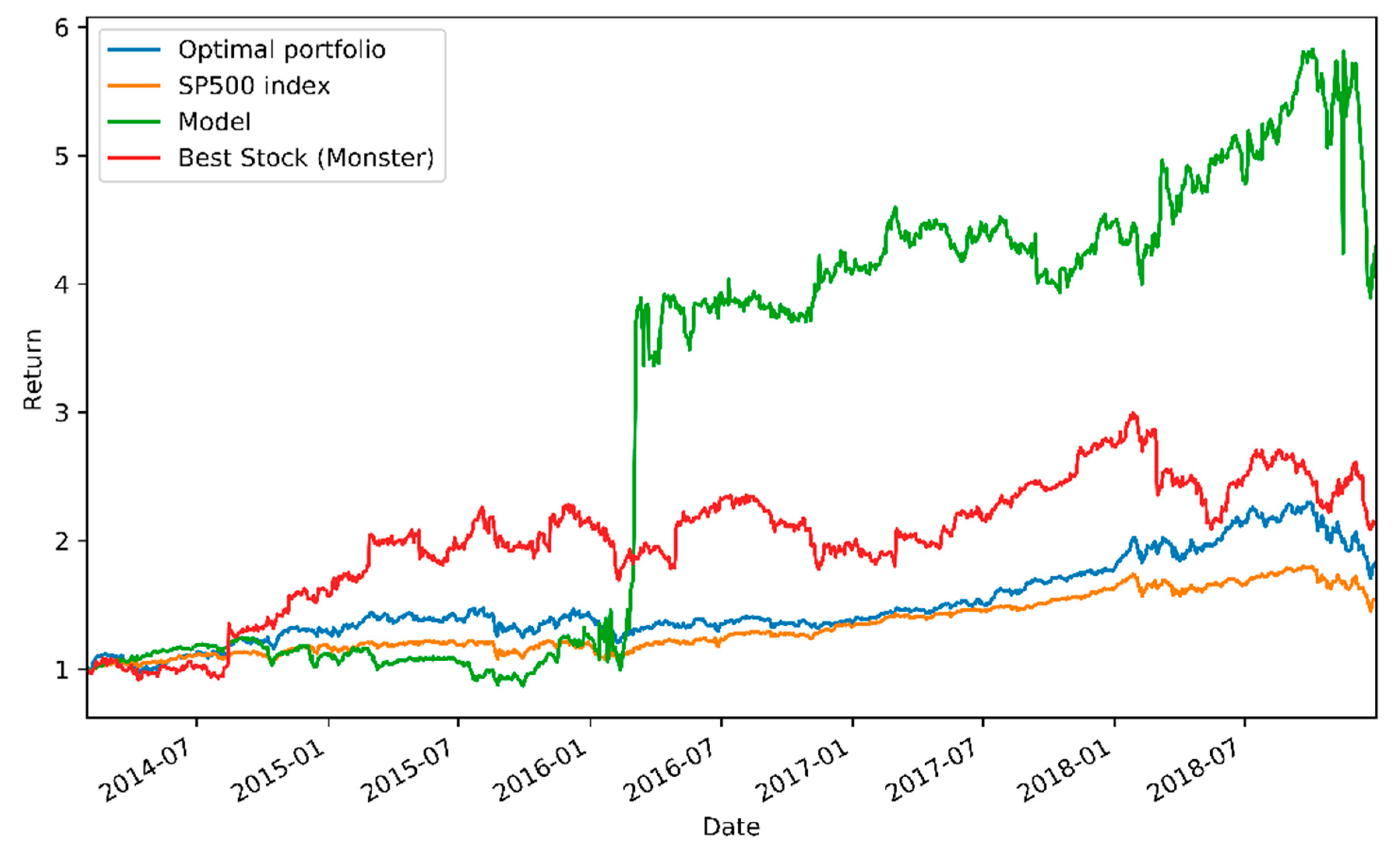
Out of the tested benchmarks, the model achieved distinctly the highest total return (328.9%) for the test period. Although the total return for the model was overwhelming, its risk-adjusted performance measured with the Sharpe ratio suggests only a slight superiority of the model. Daily standard deviation measures the riskiness of the portfolios, and it can be noted that the portfolio controlled by the model possesses the highest risk of all the portfolios, exceeding even the single-stock portfolio. To refine the insights further, the relative performances of the tested models are plotted as a function of time in Figure 2, where the high volatility of the model’s performance can be clearly seen.

From Figure 2, it can be observed that during the first 21 months, the model failed to generate excess returns and lost in performance to the benchmarks. However, during 22–28 months, the model generated rapidly very high returns and was after that able to beat the market index until the general market collapse appeared at the end and the model suffered a severe breakdown in returns.

Statistical Significance of the Results

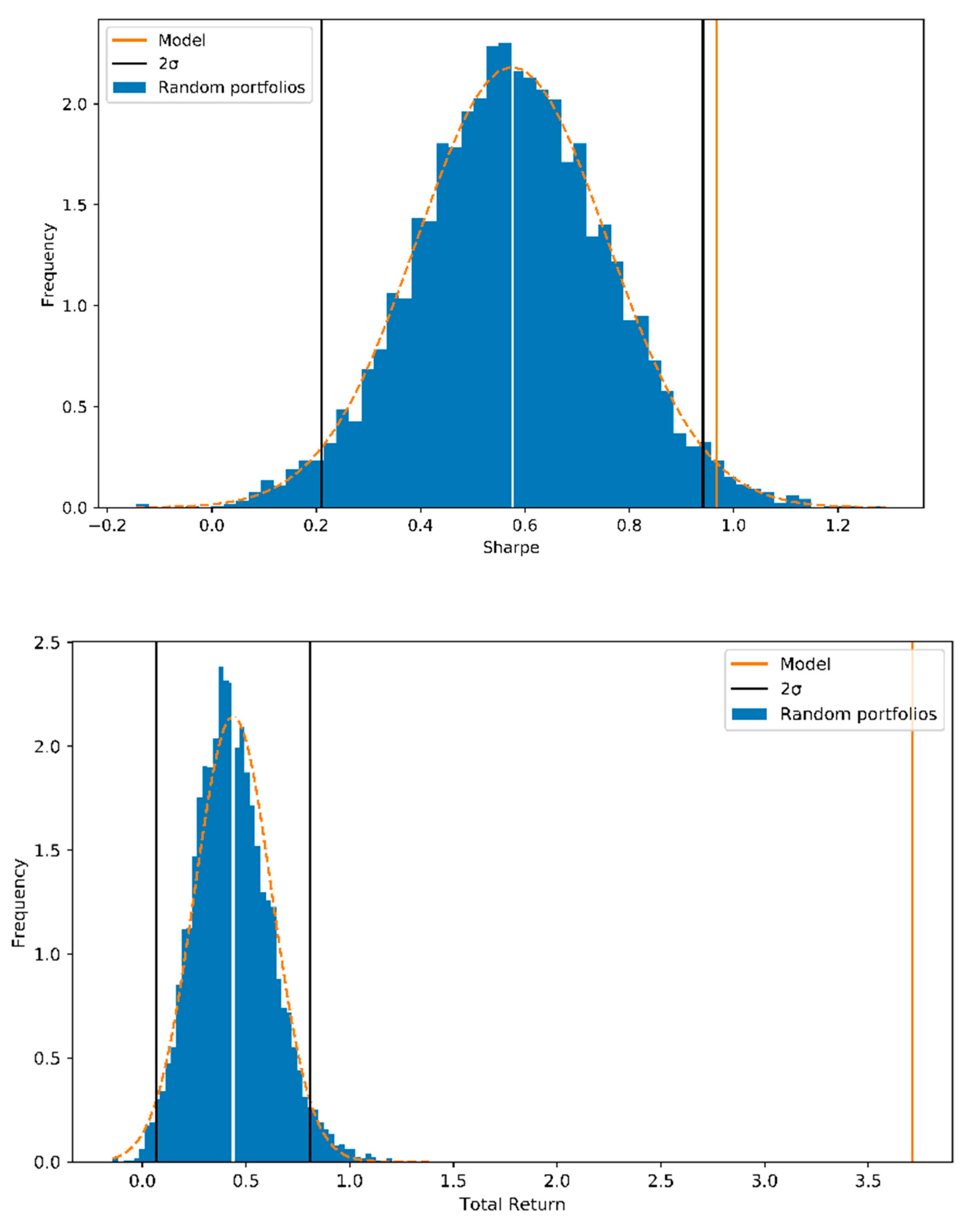
The agent model performance was statistically tested by comparing the achieved Sharpe ratio and total return to 5000 random portfolios with similar risk levels as the test portfolio. The test was conducted with a full 415 stock portfolio to minimize the effect of randomness on the portfolio performance. The random portfolios were generated to hold a similar risk profile than the trained model by allocating approximately 95% of wealth to the 200 most attractive stocks of which 11% was allocated to the most attractive stock. Figure 3 shows the performance of random weight portfolios with a full set of 415 stocks compared to the final model performance. The model achieves a Sharpe of 0.96 with the test set, and the performance exceeded the average random portfolio performance by slightly more than two standard deviations (2*σ).

The total return of the model during the test period was 370%, which exceeded the average of the random portfolios by over 16 sigma. The model improved the portfolio’s performance in a statistically significant way.

Statistical significance of the generated alpha against the S&P 500 Index was tested with linear regression and the results are displayed in

Table 4. Regression results: agent model versus S&P 500.

	Daily Returns				Monthly Returns
	Coefficient	Standard Error	t-Test	p-Value	Coefficient	Standard Error	t-Test	p-Value
Alpha	0.00117	0.00076	1.52936	0.12643	0.01747	0.02823	0.61898	0.53827
Beta	1.28613	0.09129	14.08837	0.00000	3.03349	0.80152	3.78466	0.00036

. A regression to explain the model’s returns with the market returns was executed on a daily and a monthly level. Both regressions suggest a low alpha coefficient for the model which, however, was not statistically significant since the p-values from the t-tests for both regressions exceeded the 5% risk level. Analyses indicated a high beta for the agent model.

5.3. Analysis of the Model’s Behavior

By looking at the contents of the portfolios, it can be observed that the agent did not hold all of the stocks equitably, but instead it favored certain stocks which it bought and held very frequently. Furthermore, the position taken by the agent with these favored stocks was often very close to the all-in position. To better understand this rather hazardous behavior of the agent, the states leading to the most aggressive actions by the agent were further analyzed.

It was observed that the agent preferred very volatile stocks, in which both high positive and negative returns were interpreted as a buy signal. Another and very surprising note from the states is that the agent was taking high positions to stocks with unnaturally low EP ratios, occurring mostly after an extraordinary collapse in the stock price. The performance of the agent is largely explained by this bias towards extremely low EP stocks during the test period. Clearly, this adopted strategy possessed a very high risk. The riskiness was confirmed, for example, by the fact that two of the three highest positions led to very high negative returns and, in general, the selected portfolio experienced very high positive and negative returns throughout the test period. The daily standard deviation of 3% shows that the agent practically failed to manage the risk in the portfolio and mainly focused on the very high returns while maximizing the Sharpe ratio.

During a six-month period from January 2016 to June 2016, the agent’s performance suddenly increased vastly. During this period, the agent took several all-in positions to a few different low-EP and highly volatile stocks and was able to benefit from these risky actions enormously. It was remarkable that the agent generated a major part of its profits during this six-month period.

A key explanatory factor for this risky behavior seems to be the survival bias in the training set of the S&P 500 stocks used in this study. Since the data set included companies belonging to the S&P 500 index in 2013, it excluded companies that went into bankruptcy or were excluded from the index due to the fact of weak performance before 2013. Therefore, the agent only observed companies during the training part that were able to get over the losses (of the previous crash) and to grow enough to be a constituent of the S&P 500 Index in 2013. Thus, the agent did not consider the extremely low EP ratio as a warning signal but instead as a chance for very high positive returns in the future.

In this study, the size of the portfolio picked by the agent was constrained to twenty stocks. Managing a portfolio of this size might not be the optimal way to maximize future returns, since the continuously changing portfolio was impairing the returns due to the transaction costs. The practicality of the agent could be improved by reducing the portfolio size to, for example, one stock only, and investing the rest of the wealth into the stock index.

6. Summary and Conclusions

This paper explored the applicability of machine learning models to active portfolio management using models based on deep reinforcement learning. The agent developed in this study was able to self-generate a trading policy that led to an impressive 328.9% return and a 0.91 Sharpe ratio during a five-year test period. The agent outperformed the benchmarks and was proven to improve the Sharpe ratio and total return of the stock portfolio in a statistically significant way. However, the alpha generated by the agent against the S&P 500 index was not shown to statistically differ from zero; thus, it cannot be stated that the agent model used can surpass the market return statistically significantly. The trading policy was found to possess high risks and to be very opportunistic by generating high profits with individual trades rather than by beating the index daily (and consistently). The results suggest the applicability of deep reinforcement learning models to portfolio management and thus are in a line with the results of several previous studies [18,19,20,24] that indicate the usefulness of deep learning models in this area of finance.

It was observed that a relatively simple convolutional neural network model can achieve good performance in the case of automated investing based on historical financial data. This suggests that, from a machine learning point of view, financial data are not impossible to handle, and the results of this research indicate that the patterns in the data are not very complex, if compared to, for example, image data. Financial data are noisy, and it may be the reason why using supervised learning methods have not been very successful in the past.

The results of this study are limited by the survival bias of the applied S&P 500 data set, as the companies that underwent bankruptcy during 1998–2012 were excluded from the data set and, thus, encouraged the opportunistic behavior of the agent built. Another limitation and explanatory factor for the results was the size limitation of the agents’ portfolio, which was defined in the range of zero to twenty stocks. Other issues include the length of data—21 years in this study—and which might be unnecessarily long for a single model. The importance of overall market behavior twenty years ago may be questioned when considering the current market behavior. We point out and acknowledge that the results attained in this research are tied to the market data the agent model was fitted with. Generally speaking, the agent can be used on any market data, but the results depend on the data.

To deal with the specific issues of using long-term data, the model could be trained and tested with multiple, shorter periods to determine if it benefits from more recent training data; this would possibly give a different point-of-view with regards to the robustness of the model presented and perhaps would give a different perspective about the abilities of the model as a whole. A need for further testing with shorter periods was highlighted by the model’s behavior during the rather short period during which the model was the most successful and during which the “gamble” the model took payed off. It would be most interesting to find out the market circumstances in which the model was able to produce the best results and, contrarily, where it failed to perform well.

Furthermore, future research should consider a more structured approach for both feature selection and hyper-parameter selection. These were not done exhaustively in this research; exhaustive optimization-oriented parameter selection demands a lot of computing power and requires the construction of an automated system for running multiple parameter combinations to find the overall best parameters.

As a final note, since the stock market is an extremely noisy environment, the trader agent could benefit from a lower trading frequency that lengthens the holding period of a single stock and, thus, protects the model from drawing wrong conclusions in the short term. Relaxing these above assumptions and running a larger sensitivity analysis is left for future study.