1. Introduction
The Traveling Salesman Problem (TSP) is one of the most classic NP-complete graph search problems (Non-deterministic Polynomial time problems) with many real life applications, particularly, in transport and logistics. The Time-Dependent Traveling Salesman Problem (TD TSP) is an extension of the classic TSP towards more realistic traffic conditions [
1]. The total cost of any salesman’s (round) trip consists of two main elements: Costs proportional to transit distances (as in the original TSP) and costs added by increasing transit times (caused by traffic jams occurring in rush hour periods in certain areas of the route). Although the physical distances and, thus, the theoretical costs between a pair of nodes (cities, shops, etc.) can be considered as constant, the real transit times are subject to external and environmental factors, such as weather conditions, traffic circumstances, unexpected factors like road construction and accidents, etc. So, they should be treated as time dependent but also as uncertain variables, in particular, as time-dependent fuzzy cost coefficients. However, in the original model of the TD TSP, the edges are basically assigned fixed weights (costs), which are either multiplied or not by a “rush hour factor”, depending on whether they are traveled within the specific traffic jam region(s) and during the fixed rush hour period(s).
Even though this is more real-life style than the basic, abstract TSP, this representation is still far from the full reality, because of the following two phenomena.
The different traffic regions might (partially) overlap. Usually, they do not have any crisp, well-defined borders and it is never known if any nondeterministic outside effect does not modify the actual cost, which all point at the fact that a rather complex and ambiguous time-dependent cost value is associated with each edge. This problem is obviously not addressed properly in the classic TD TSP model proposed by Schneider [
1], a clear justification for further extensions of the existing model.
Similarly, the effects of the rush hour(s) are presented by simple crisp numbers and they are taken into consideration only during certain fixed time intervals (a single interval in the original model cf. [
1]), which is far from the complexity of real-life situations. Rush hours have a dynamic nature; they usually build up gradually and also disappear gradually, although they can occur quite fast due to a random road accident or because of the start of a road construction. (This problem is one of the classic examples that Prof. Zadeh often mentioned in his plenary lectures by the question “How much time does it take from my Berkeley home to San Francisco Airport?”). Thus, it seems a rather reasonable approach to look at jam regions and rush hours as uncertain areas (of space and time) and represent them by additional cost components, and to represent those using fuzzy numbers and fuzzy sets.
2. An Overview of the Literature of the Extensions of the TD TSP
In the research of the TD TSP group, there have been several attempts to efficiently quantify the contribution of the jam regions and the rush hours to the cost in an actual road trip. We categorized those efforts in two groups: Non-fuzzy extensions and fuzzy model-based extensions, where our main contribution belongs.
2.1. Non-Fuzzy-Based TD TSP Extensions and New Algorithms
In 2016, Taş et al. proposed a variant of the Traveling Salesman Problem with time-dependent service times [
2]. The mathematical formulation of the model was extended with sub-tour elimination constraints and was solved by using IBM ILOG CPLEX 12.5. The tests were carried out only on smaller instances up to 45 nodes. Even for these relatively small graphs, in quite many cases the optimal solutions were not found within the time limit set by the authors (7200 s).
In 2016, Hurkała proposed a new algorithm for the TD TSP with multiple time windows and compared it with three well-known and often efficient heuristic methods (simulated annealing, list-based threshold accepting algorithm, and variable neighborhood search) [
3]. The main drawback of these results is that the methods mentioned were tested on even smaller instances, up to 23 nodes only, although these heuristic approaches were able to handle larger instances, as it was shown in a multitude of other papers reporting on meta-heuristic solutions of various other TSP-related graph search tasks.
In 2018, Vu et al. presented an integer programming formulation for solving the TD TSP with time windows. However, this approach was again only able to solve small instances, up to 40 nodes [
4].
In 2018, our team also published a novel (non-fuzzy) approach, where a parameter-adapted version of the rather generally applicable (say, “universal”), efficient, and efficacious method called discrete bacterial memetic evolutionary algorithm (DBMEA) was applied for solving the problem, first, for the reason of possible comparison, on Schneider’s instances. The proposed meta-heuristics clearly outperformed previous attempts for the solution of this problem, and, by adding a number of new, larger instances, it was also shown that DBMEA did not have restrictions concerning the size of the graph (rather, when knowing the size, a good prediction of obtaining a good approximate solution could be obtained).
In 2019, Ban proposed a two-phase meta-heuristic algorithm [
5] for Schneider’s version of the Time-Dependent Traveling Salesman Problem, but it did not outperform the earlier published DBMEA approach [
6].
Also in 2019, Vu et al. proposed an integer programming approach which was based on an integer programming formulation of the problem on a time-expanded network. This novel technique outperformed the best-known methods on the benchmark instances [
7] and, thus, this may be considered now as “best practice” in a certain sense. However, while Vu’s algorithm is a clear competitor of the DBMEA concerning speed and accuracy, it is still a tailor-made technique with a very narrow applicability scope that cannot easily be adapted to any extension or generalization of the original problem and, thus, it may not be considered as universal (generally applicable). Also, the (rather important) predictability of the expected run time for optimizing a given size problem is not good. In the attempt of extending the model towards more complex, fuzzy, etc. graphs and searching for an efficient algorithm for acceptably good approximate solutions of instances of this extended model, it was obviously important to have some generally applicable approach that promised good results even for new, more general problem classes with unknown, potentially unexpected behavior (For the investigations concerning the general applicability, called universality, of the DBMEA algorithm family, cf. [
8]).
The extensions mentioned above are more general and more realistically applicable compared to the original TSP. However, these models do not take into account the inherited uncertainty involved in real life situations as mentioned above (such as the uncertainty of the distances (costs) between the pairs of nodes, the uncertainty of the time-dependence periods, the uncertainty of the geographic extensions of the traffic jam areas, or the uncertainty of the time windows (TW) in the further extended TD TSP TW).
Finally, it should be mentioned that several further meta-heuristic alternatives for solving the TD TSP have been proposed which yield generally efficient approaches. The most promising one was proposed by Roy et al. [
9], but it has a serious disadvantage than applying the original genetic algorithm for the base of the memetic approach, which has been shown in numerous investigations to be inferior to the bacterial evolutionary algorithm, being considerably slower and less accurate [
10].
2.2. Fuzzy Model-Based TD TSP Extensions
Despite the promising results achieved so far by various researchers in determining the minimal overall tour cost for the TD TSP, a major drawback is the simplification in representing all factors connected with the phenomenon of potential traffic jams and other nondeterministic effects and the neglecting of uncertain issues influencing the actual costs between nodes originally modeled by crisp singleton values. We propose that this pitfall was overcome to various extents in all three of our novel fuzzy-based approaches for the TD TSP with jam regions and rush hours. Indeed, in each of the three models we introduced, we moved gradually one step forward in representing the uncertain circumstances in the jam regions and during the rush hours more precisely.
2.2.1. The Triple Fuzzy TD TSP (3FTD TSP)
In the
Triple Fuzzy (3FTD TSP) model, the costs of the edges between the pairs of nodes depend in an uncertain and nondeterministic way on the time and location; and those vague values are expressed by fuzzy sets [
11]. In the practical model, these uncertainties were represented by simple trapezoidal fuzzy numbers. Jam regions were also defined as fuzzy regions within the metric space, where the graph was embedded. On the other hand, the rush hour times were considered as bimodal normal fuzzy sets (one for each jam region), based on data coming from real traffic measurement databases. We claim that the 3FTD TSP model expressed well the uncertain costs influenced by the traffic jam situations and ultimately calculated the overall tour length quantitatively, but with all the mentioned uncertainties being taken into consideration. We are convinced this first fuzzy TD TSP model simulated real-life situations more adequately than the original crisp one [
11].
2.2.2. The Intuitionistic Fuzzy TD TSP (IFTD TSP)
Further consideration of the uncertainty factors was done when we proposed the
Intuitionistic Fuzzy TDSP (IFTD TSP) model [
12]. The concept of intuitionistic fuzzy sets (IFS) was introduced by Atanassov [
13] as another type of generalization of the concept of fuzzy sets since, in reality, it is not always true that the degree of nonmembership of an element in a fuzzy set is equal to one minus the membership degree, because there may be some hesitation degree. That concept is well addressed in IFS that incorporates the degree of hesitation, which is defined as one minus the sum of membership and nonmembership degrees. Adding a hesitation part to either the membership value or to the nonmembership value (or to both) assigned to the local and temporal embedding of the cost factors allowed a higher level involvement of the complex nature of uncertainty, say, the secondary uncertainty originating from the subjectivity and partly the random sampling of cost-influencing factors [
13]. Let
A be an IFS in
X, an object having the form
where
.
The amount is called the hesitation part, which may cater to either the membership value or to the nonmembership value or to both. The underlying main concept behind the IFTD TSP model was conducted using the IFS theory to represent the uncertainty of jam regions and rush hours in a tour. In brief, let X and Y be two IFSs. An intuitionistic fuzzy relation (IFR) R from to Y is an IFS over Y characterized by the membership function and nonmembership function . An IFR R from X to Y will be denoted by . If the state of the edge E is described in terms of an IFS A of J (over the universe X). Then E is assumed to be the assigned cost expressed by IFS B of C (over the universe X) through an IFR R from J to C, which translates the jam degrees of association and non-association according to geographical areas on the destination cities and the extent (membership) to which each one is included in the jam region. This will be translated to the degrees of association and non-association, respectively, between jam regions and costs as follows.
For
n edges
,
i = 1, 2, …
n in a tour (from the starting node to the destination node) and
, let
R be an IFR
and construct an IFR
from the set of edges
E to the set of jam factors
J as
. The max-min-max composition [
14]
T of IFRs
R and
Q is used to calculate the cost for each edge from
E to
C, given by the membership function
and the nonmembership function given by
The use of intuitionistic, instead of traditional fuzzy, sets provided an even more sensitive and realistic cost estimate for the tours, influenced by the jam factors and rush hours, thus simulating real-life scenarios of the TD TSP problem.
2.2.3. The Interval-Valued Intuitionistic Fuzzy TD TSP (IVIFTD TSP)
Despite the essential extension of the original abstract model and the inclusion of uncertainties, the previously mentioned IFTD TSP approach has some drawbacks, namely, the properties of the max-min-max composition that was used in Equations (2) and (3), when determining the ultimate costs of the rush hours and jam regions of a tour (explained
Section 2.2.2). The result of this composition operation is only affected by the extreme values and ignores the smaller values of the jam regions and the rush hours, which might be considered problematic. In fact, the cost calculation using this operation leads to quite conservative results because it does not cater for all the jam regions and rush hours costs. On the contrary, it takes into consideration only the largest values and neglects the rest, leading to more information loss. A mathematically more adequate solution would be aggregating the traffic jam factors by a strictly monotonic operation and applying a corresponding relational operation as well, rather than executing the max-min-max composition. Such a new approach seems to offer more interpretable results. This last observation was the main turning point in proposing the present new IVIFTD TSP model. But first we will go through some preliminary definitions and how the model was built.
3. Interval-Valued Type-2 Fuzzy Sets
Here, a brief overview of the tool kit used in this model will be given. Since Zadeh [
15] introduced fuzzy sets in 1965, there have been many approaches and theories introduced to treat imprecision and uncertainty more adequately. Generally, classical, type-1 fuzzy sets are not able to directly model complex uncertainties adequately, because their membership functions assign crisp values to the membership degrees and, thus, the measure of uncertainty is “rigid”. On the other hand, type-2 fuzzy sets model uncertainties more efficiently, because their membership functions assign degrees which are fuzzy themselves [
16]. The membership functions of type-2 fuzzy sets are (
n + 2)-dimensional, while membership functions of type-1 fuzzy sets are only (
n + 1)-dimensional (assuming that the universe of discourse has
n dimensions). Thus, type-2 fuzzy sets allow more degrees of freedom in representing uncertainty.
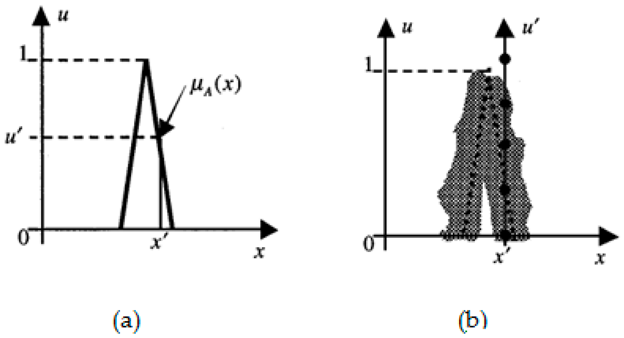
To illustrate, as Mendel explained in his work [
16], if we blur type-1 membership function (see
Figure 1a) by shifting the points on the triangle left or right we get the membership function in
Figure 1b. Then, to a specific element of the universe, no longer is a single value assigned as membership degree; instead, the membership function assumes all values where the “vertical” line intersects the blur. (In the figure, we have given those values equal weight as explained in the numerical example later.) This additional degree of freedom conveys new information (see
Figure 2), which offers more control on the effects of uncertainties and vagueness in rule-based fuzzy systems and, thus, makes it possible to directly model uncertainties [
16], which, in turn, will allow a more adequate simulation of any phenomenon that contains a considerable amount of vagueness and/or inconsistency. This is very useful when uncertainties affect the nature of specific problems and provides better performance [
16], especially, in modeling real-life situations. A prime example may be modeling the traffic conditions in urban areas for the TD TSP. The uncertainty of the membership function in type-2 set
in Equation (4) consists of a rounded region called “footprint of uncertainty” (FOU), the union of all primary memberships.
FOUs emphasize the distribution that sits on top of the primary membership function of the type-2 fuzzy set. The shape of this distribution depends on the secondary grades. When they all equal 1, the resulting type-2 fuzzy sets are called interval type-2 fuzzy sets that take the form as in Equation (5).
Indeed, due to the increased computational complexity of applying general type-2 fuzzy sets, a compromise is often accepted to reduce computational needs, namely, the application of
interval type-2 fuzzy sets. This simplification of the third dimension of the membership function makes mathematical operations more manageable. Since TD TSP is known as an NP hard problem itself [
1], modeling it by general type-2 fuzzy sets will just increase the complexity further. Thus, it is more manageable from the complexity point of view to apply interval type-2 and, in addition, interval type-2 fuzzy sets offer a quite practical and tractable model while the double uncertainty feature is still preserved [
16,
17].
4. The Interval-Valued Intuitionistic Type-2 Fuzzy Sets Model (IVIFTD TSP) and the Optimization Approach
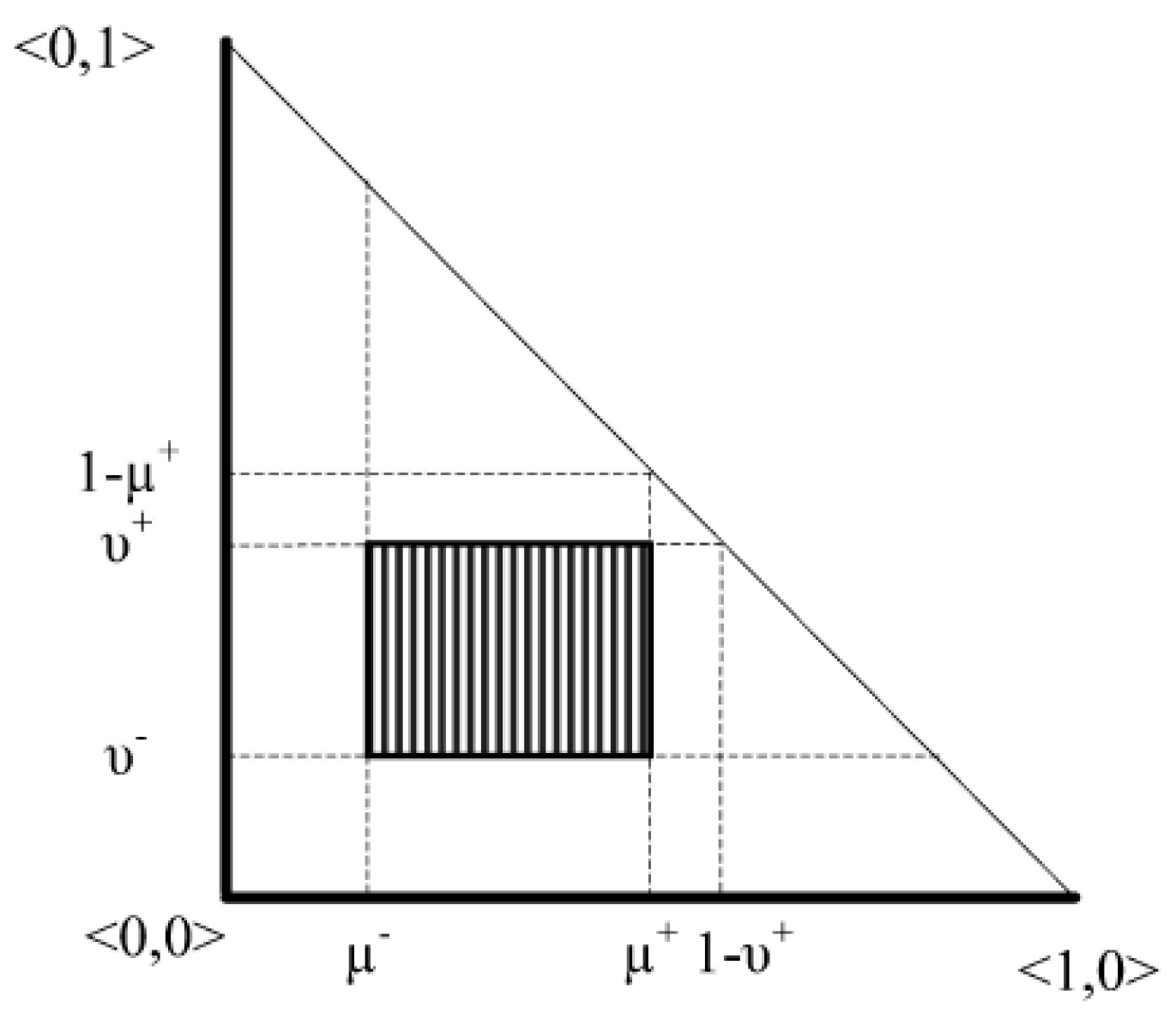
Atanassov and Gargov [
13] defined the concept of interval-valued intuitionistic fuzzy sets (IVIFS), as well, in 1989, which is a further generalization of the definition of the IFS [
14]. Each IVIFS is characterized by a pair of a membership function and a nonmembership function whose values are intervals rather than real numbers. The IVIFS (
Figure 3) is more powerful in dealing with multiple and complex vagueness and uncertainty than the plain IFS, because it incorporates the hesitation degree (hesitation margin) in calculating the membership function by using the new, third dimension of type-2 fuzzy sets, thus combining the two powerful features of IFS and IVFS. Modeling problems with high uncertainty and hesitation via IVIFS look more promising in terms of capturing the intangible vagueness factors and their numerical effects. Also, IVIFSs decrease the information loss that comes from using IFSs solely. Indeed, IVIFSs have received much attention from researchers concerning how to deal with the interval-valued intuitionistic fuzzy numbers (IIFNs), which is the basic point of using IVIFS. In the literature, many ideas were presented to address the definition of some proper interval-valued intuitionistic fuzzy aggregation operators. Xu and Chen [
18,
19] proposed several arithmetic aggregation operators for IVIFSs, such as the interval-valued intuitionistic fuzzy weighted arithmetic mean aggregation (IIFWA), the interval-valued intuitionistic fuzzy ordered weighted mean aggregation (IIFOWA), and the interval-valued intuitionistic fuzzy hybrid aggregation (IIFHA). Xu and Chen [
20,
21] also introduced the interval-valued intuitionistic fuzzy weighted geometric mean (IIFWG), the interval-valued intuitionistic fuzzy ordered weighted geometric mean (IIFOWG), and the interval-valued intuitionistic fuzzy hybrid geometric mean (IIFHG) operators. In our model, it was convenient to apply the IIFWA definition (see Equation (8)), to accumulatively calculate the jam region and rush hours’ costs assigned to the edges.
For a universal set
X, an IVIFS
A is an object having the form as in Equations (6) and (7).
where
represent the degree of membership and nonmembership, respectively, and
Let any n IVIFSs
be a collection of interval-valued intuitionistic fuzzy degrees. Then, an IIFWAA operator is defined in Equation (8)
where
are the weight vectors of
A. Further,
and
(In our simple model, we gave equal weights to all the jam factors by
).
Lastly, for finding the final jam factor cost, we used a measure based on Park’s distance between IVIFS. Finding the distance between IFS has attracted many researchers as an alternative to the max-min-max composition. Park et al. [
22] proposed new distance measures between IVFSs based on the Hamming distance. We adopted the normalized Hamming distance considering the hesitation part as in Equation (9).
For any
and
)
where
H is the hesitation part.
In the IVIFTD TSP, the jam factor costs of the edges in a tour were represented as fuzzy relations between the jam factors and the predicted edge assigned costs (delays caused by the traffic jam phenomena). Let
,
and
denote the sets of jam factors, costs, and edges, respectively. We will introduce two fuzzy relations:
Q that is defined over set
Equation (10), and
R that is defined over set
as in Equation (11).
where
indicates the degree to which jam factor
j affects edge
e, while
indicates the degree to which jam factor
j does
not affect edge
e. Similarly,
and
are the relationships between jam factors and the respective costs. (This is what we refer to as
confirmability degree in the coming sections). Thus,
and
represent the degrees to which jam factor
j confirms and does not confirm the presence of cost
c, respectively. Since
Q is defined over set
and
R over set
, the composition
T of
R and
Q (
) for prediction of the cost for a specific edge can be represented by
FR from
E to
C, given the membership function in Equation (12) and nonmembership function in Equation (13).
for all
.
In
Section 4.2 we apply the proposed approach on a real-life TD TSP cost problem, taking into consideration the gradual buildup of rush hours and the uncertain geographical extent of the jam regions. The approach consists of four stages:
Stage 1. Calculate a prediction for the rush hours and jam regions of the edges, in the sense that if the trip between the two cities happens during the rush hours and within the jam regions, both will be taken into consideration and none of the factors will be neglected.
Table 1 identifies the cost of each jam factor, which is supposed to be predefined by experts in this domain, according to the rush hours and the jam regions of the city of study.
Stage 2. Calculate the interval-valued intuitionistic fuzzy weighted arithmetic average (IIFWAA) of the confirmability and nonconfirmability degrees of the edges using aggregation in Equation (8). Normally, jam regions and rush hours affect different edges within a tour simultaneously, but in different degrees. In this case, we need to aggregate the interval-valued intuitionistic fuzzy information corresponding to the degrees for the edge jam factors and the confirmability degrees.
Stage 3. Calculate Park’s distance between the IFSs using the IIFWAA obtained in Step 2. (See Equation (9).)
Stage 4. Determine the final jam factor costs (caused by the rush hours and jam regions) based on the measured Park’s distance in the third stage (The weights can be assigned according to the topography and importance of the routes. In our case we simply assumed equal weights for all factors).
4.1. A Simple IVIFTD TSP Application Case Study
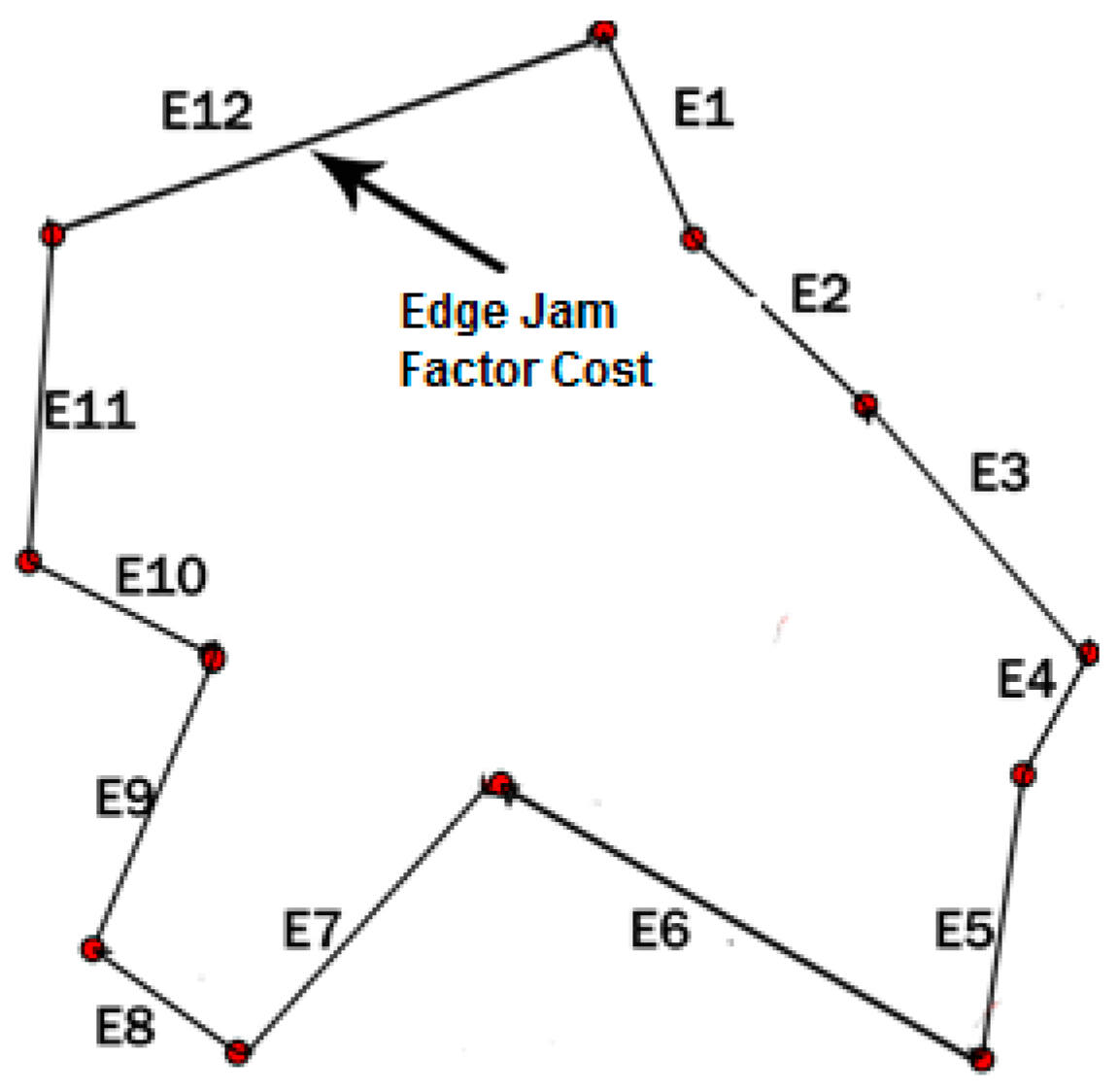
In this section, we present an example to illustrate how to apply the proposed new model on a simple TD TSP case study with double uncertain jam regions and rush hours. Let us consider that
E1 is the first edge of a tour, as in
Figure 4. In the case study, there are four different traffic factors assumed (which may be jam regions and/or rush hour periods) affecting
E1 simultaneously. In the illustration we use
estimated by domain experts who were able to define the degree on how a jam factor
j affects edge
e, as in Equation (10), and the nonconfirmability degree, as in Equation (11). The jam factors of
E1 affecting that edge in the example are (1.1, 1.2, 1.3, 1.4, 2.1, and 2.2), which are all related to a specific cost (delay), as shown in
Table 1.
Table 2 shows the jam factors assigned to edge 1 (
E1).
Table 3 gives the confirmability and nonconfirmability degrees with jam factors (1.1, 1.2, 1.3, 1.4, 2.1, and 2.2), according to their degrees of belonging to the rush hour periods and jam regions (referred to from here as “traffic factors”, as a generalized term).
Table 3 gives confirmability degrees for
E1, which is extracted from the general knowledge base represented in
Table 1.
Step 1. Based on
Table 2 and
Table 3, we calculate the results in
Table 4 and
Table 5 by applying the IIFWAA operator on
,
in
Table 3 (see Equation (8)). For example, [0.61, 0.71], an IIFWAA
of
Table 5, is calculated as follows (
bolded in the first two columns of
Table 3): The confirmability membership degrees of the edge jam factors (1.1, 1.2, 1.3, and 1.4) are ([0.6, 0.7], [0.6,0.7], [0.5, 0.6], and [0.7, 0.8]), and here the first edge is affected by four jam factors,
and so the distributed weight is calculated as
as follows
in
Table 5 is calculated as follows: Take the confirmability values for the nonmembership degrees of the jam factors [0.1, 0.2] [0.2, 0.3] [0.1, 0.2] [0.1, 0.2] and apply IIFWAA, as below
Step 2. Calculate Park’s distance by applying Equation (9), taking values from
Table 4 and
Table 5.
Step 3. Find the lowest distance between IVIFS, because it points out the jam factor that is causing the highest delay and, thus, the one worth considering (in our case this is 0.16, as shown in
Table 6). As a result, we can infer that
E1 is affected preferentially by cost1 (0.16) and, hence, causing the largest delay in that edge. If we carry on with the same calculations for all the edges, we reach the data presented in
Table 7 that shows all the jam factor costs for the edges, depending on their respective confirmabilities.
After observing the results in
Table 7 from the numerical example, we may notice that applying the IVIFTD TSP with rush hours and jam regions was done by aggregating the information of the degrees of belonging and not belonging of a specific node. Thus, all jam factors were taken into consideration and none of the factors’ effects were neglected. In addition, using Park’s distance of IVFS data to reduce the loss of information led to more accurate calculations compared to our previous approach with considering less complex uncertainty, namely, the IF TD TSP [
12]. The IVIFTD TSP approach can be applied in many related areas with similar time-dependent traffic conditions, especially in logistics and transportation, like single and multiple vehicles routing (VRP) and industrial supply chain planning.
4.2. Advantages of the IVFTD TSP Model
The modeling of complex uncertainty by applying Interval-Valued (Type-2) Intuitionistic Fuzzy Sets may lead to a rather realistic and adaptable model that offers several advantages:
This model is suitable for real-life situations when cost is uncertain and unpredictable due to the influence of unknown and nondeterministic circumstances in many day-to-day situations in transport and logistics. Another major advantage is that if we want to find the optimal solution for such problems, we must compare a large number of other methods. Nevertheless, if the newly proposed model gives a good enough solution in an efficient manner, then it may definitely be considered as a good extension of the TD TSP
The prediction for the rush hours and jam regions is done by aggregating the information on the degree of belonging and not belonging of a specific node to the jam regions or rush hours, i.e., if the trip between the two cities is happening during the rush hours and within one of the jam regions, both will be taken into consideration according to their weights and none of the uncertainty elements will be neglected.
Using the concept of Park’s distance of IVFS data in order to reduce the loss of information takes into consideration all jam factors and rush hours that might affect an edge in a specific period of time (not only the extreme values of those factors).
The preliminary information knowledge base proposed in the model about the main regions for rush hours and jam regions (which allow deciding whether a particular edge belongs to that area or not) makes this approach easily applicable in practice and automated through a computer program module.
5. Computational Results
Schneider tested his simulated annealing algorithm only on the bier127 instance, however, with various jam factors. Li et al. also examined their record-to-record travel algorithm on the bier127 problem [
23]. As a continuation of this effort, in order to have some directly comparable results, we also tested Schneider’s simulated annealing approach for solving the interval-valued intuitionistic fuzzy model. We have taken cost factors that represent the shortest distances for a tour (as explained in
Section 4.1). Although the simulated annealing was very fast (because it is not a population-based method, it works by improving one single candidate solution), the DBMEA [
6] found considerably better solutions for the IVIFTD TSP. As mentioned before, the DBMEA is a combination of the bacterial evolutionary algorithm [
24,
25] as global search and a sped-up version of 2-opt with subsequent 3-opt as local search [
6]. The local search usually improves the performance significantly, in terms of algorithm speed and accuracy.
Table 8 shows the test results of the DBMEA and the simulated annealing approaches on the bier127benchmark problem with various jam factors. The results demonstrate the effectiveness of the DBMEA algorithm. Comparing the DBMEA results with the simulated annealing, in all cases the DBMEA found the same tours as the simulated annealing, yet gave better performance.
6. Conclusions
In this paper, the interval-valued intuitionistic fuzzy sets’ extension was applied to construct a more accurate model of the realistic Time-Dependent Traveling Salesman Problem, where the multiple uncertainties of the jam regions and rush hour periods could be adequately included in the model. In order to be able to test and compare the new model with the original one, we developed a small repository with interval-valued type-2 fuzzy degrees based on the relations among jam regions according to closeness of city centers and rush hours during the day and their estimated costs in terms of the elapsed time (additional delay) during the passing of the sections. Those costs essentially affect the overall tour length (tour cost or time) and even the topography of the optimal tour. To efficiently combine the interval type-2 and the intuitionistic values, we utilized the interval-valued intuitionistic fuzzy weighted arithmetic average operator to aggregate interval-valued fuzzy information resulting from the various jam-related factors. We also proposed a measure based on Park’s distance between IVIFS for the TD TSP cost under such circumstances. The results of the example indicated that the new model is effective while it simulates real-life conditions and successfully quantifies the traffic-related effects without essential loss of information. We expect that this model will give more tangible treatment of such uncertain factors and, thus, it offers better modeling accuracy and flexibility than all previous models in the literature. In the past, we worked on various level realistic extensions of the TD TSP and proposed two fuzzy model-based methods: The Triple Fuzzy Model for the Time-Dependent Traveling Salesman Problem and The Intuitionistic Fuzzy Model for the Time-Dependent Traveling Salesman Problem. Continuing this research, in this paper an even more advanced approach was introduced: Interval-Valued Intuitionistic Fuzzy Model for the Time-Dependent Traveling Salesman Problem.
Future work will focus on testing the model on larger instances and more complex transportation problems with various jam areas and rush hour conditions. However, the successful optimization of even TD TSP instances orders of magnitude larger, even though of less complex uncertainty, is very promising and we are convinced that the “universality” of the optimization meta-heuristics will guarantee quality results even for these higher complexity problem.


