Introduction
In paper [
1] we analyzed the numerical solution of the first order Ordinary Differential Equation (ODE),
associated with the initial condition:
where
is a
function on its domain and
is assigned. In particular, we considered the numerical solution of Hamiltonian problems which in canonical form can be written as follows:
with
where
and
are the generalized coordinates and momenta,
is the Hamiltonian function and
stands for the identity matrix of dimension
ℓ. Note that the flow
associated with the dynamical system (
3) is symplectic; this means that its Jacobian satisfies:
We recall that a one-step numerical method
with stepsize
h is symplectic if the discrete flow
satisfies:
Two numerical methods
are conjugate to each other if there exists a global change of coordinates
, such that:
with
uniformly for
varying in a compact set and ∘ denoting a composition operator [
2]. A method which is conjugate to a symplectic method is said to be conjugate symplectic, this is a less strong requirement than symplecticity, which allows the numerical solution to have the same long-time behavior of a symplectic method. A more relaxed property, shared by a wider class of numerical schemes, is a generalization of the conjugate-symplecticity property, introduced in [
3]. A method
of order
p is conjugate-symplectic up to order
, with
, if a global change of coordinates
exists such that
, with the map
satisfying
A consequence of property (
7) is that the method
nearly conserves all quadratic first integrals and the Hamiltonian function over time intervals of length
(see [
3]).
Recently, the class of Euler–Maclaurin Hermite–Obreshkov (EMHO) methods for the solution of Hamiltonian problems has been analyzed in [
4] where the conjugate symplecticity up to order
of the
p-th order methods was proven. In this paper, we fix Theorem 1 of [
1] related to symmetric one-step BS Hermite–Obreshkov (BSHO) methods, proving that the conjugate-symplecticity property is satisfied by the
R-th one-step symmetric Hermite–Obreshkov method up to order
.
Let
be an assigned partition of the integration interval
, and let us denote by
an approximation of
. We consider one-step symmetric BSHO method as follows, setting
where
,
, and
, for
denotes the
-th Lie derivative of
computed at
,
where
is the identity operator and
is defined as the
k-th total derivative of
computed at
where for the computation of the total derivative it is assumed that
satisfies the differential equation in (
1). Thus for example
where
is the
Jacobian matrix of
Note that we use the subscript to define the Lie operator to avoid confusion with the same order classical derivative operator in the following denoted as
With this clarification on the definition of
following the lines of the proof given in [
4], we can actually prove that the
R-th one-step symmetric BSHO method is conjugate symplectic up to order
.
We show that the map associated with the BSHO method is such that , where is a suitable conjugate symplectic B-series integrator.
Theorem 1. The mapassociated with the one-step method (8) admits a B-series expansion and is conjugate to a symplectic B-series integrator up to order.
Proof. The existence of a
B-series expansion for
is directly deduced from [
5], where a
B-series representation of a generic multi-derivative Runge-Kutta method has been obtained. By defining the two characteristic polynomials of the trapezoidal rule:
and the shift operator
the
R-th method described in (
8) reads,
We now consider a function
, a stepsize
h and the shift operator
, and we look for a continuous function
that satisfies (
10) in the sense of formal series (a series where the number of terms is allowed to be infinite), using the relation
where
is the classical derivative operator,
By multiplying both sides of the previous equation by
, we obtain:
Now, since Bernoulli numbers define the Taylor expansion of the function
and
and
for the other odd
we have:
Thus, we can write (
11) as
Adding and subtracting terms involving the classical derivative operator
, we get
that we recast as
Since
, due to the regularity conditions on the function
, we see that
and hence the solution
of (
12) is
-close to the solution of the following initial value problem
with:
that has been derived from (
12) by neglecting the sums containing the derivatives
. Observe that
for
since the method is of order
(see [
2], Theorem 3.1, page 340). We may interpret (
13) as the modified equation of a one-step method
, where
is evidently the time-
h flow associated with (
13). Expanding the solution of (
13) in Taylor series, we get the modified initial value differential equation associated with the numerical scheme by coupling (
13) with the initial condition
. Thus,
is a B-series integrators. The proof of the conjugated symplecticity of
follows exactly the same steps of the analogous proof in Theorem 1 of [
4]. Since
and
is conjugate-symplectic, the result follows using the same global change of coordinates
associated to
. □
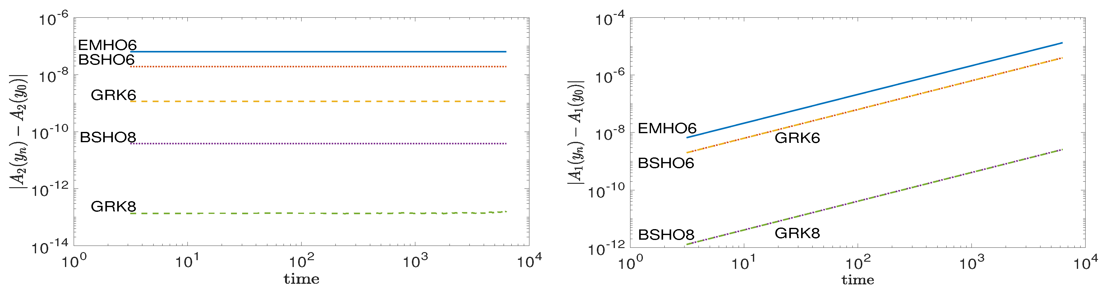
We report in
Figure 1 the bottom-rigth picture of Figure 2 of [
1], related to the Kepler problem, where we noticed that the error in the second component of the Lenz vector was not correctly computed, for completness
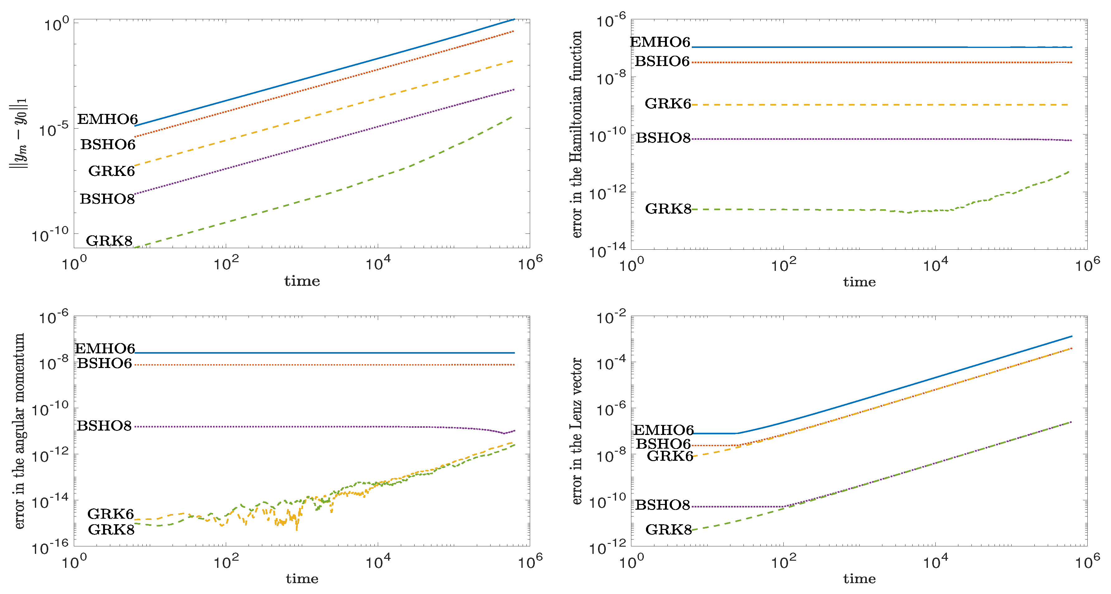
Figure 1 also reports the error in the first component of the Lenz vector. To stress that the methods show a good long time behavior for Hamiltonian problems, we report also, in
Figure 2 the results using a longer integration interval of
periods and all the other parameters unchanged. In the pictures we report the maximum error in each period for the Hamiltonian function, the angular mument and the Lenz vector. The results remain consistent, showing a linear grows in the error and in the Lenz vector and a near conservation of the Hamiltonian and of the angular moment.
All the other results in the paper do not change.


