Article

Accurate Approximations for a Nonlinear SIR System via an Efficient Analytical Approach: Comparative Analysis

Department of Mathematics, Faculty of Science, University of Tabuk, P.O. Box 741, Tabuk 71491, Saudi Arabia
Axioms 2024, 13(3), 167; https://doi.org/10.3390/axioms13030167
Submission received: 16 December 2023 / Revised: 30 January 2024 / Accepted: 6 February 2024 / Published: 4 March 2024
(This article belongs to the Special Issue Differential Equations and Related Topics)

Abstract

:
The homotopy perturbation method (HPM) is one of the recent fundamental methods for solving differential equations. However, checking the accuracy of this method has been ignored by some authors in the literature. This paper reanalyzes the nonlinear system of ordinary differential equations (ODEs) describing the SIR epidemic model, which has been solved in the literature utilizing the HPM. The main objective of this work is to obtain a highly accurate analytical solution for this model via a direct technique. The proposed technique is mainly based on reducing the given system to a single nonlinear ODE that can be easily solved. Numerical results are conducted to compare our approach with the previous HPM, where the Runge–Kutta numerical method is chosen as a reference solution. The obtained results reveal that the current technique exhibits better accuracy over HPM in the literature. Moreover, some physical properties are introduced and discussed in detail regarding the influence of the transmission rate on the behavior of the SIR model.

1. Introduction

Modeling the outbreak and spread of diseases has a long history. John Graunt [1] may have been the first to quantify causes of death systematically. However, the first mathematical model describing an infectious disease was proposed by Daniel Bernoulli [2] in 1760. Moreover, McKendrick and Kermack introduced a simple deterministic (compartmental) model describing the behavior of epidemic outbreaks in 1927 [3], known as the Susceptible–Infected–Recovered (SIR) model. Based on these works, a number of mathematical models have been developed and established under various conditions and situations [4,5]. In addition, some authors used the basic idea of the SIR model to formulate several mathematical models [6,7,8,9] to predict the behavior of COVID-19, which is an infectious disease caused by the SARS-CoV-2 virus. Various ISR models have been implemented to investigate the progress of COVID-19 in different countries [10,11,12,13,14], while other mathematical models have been developed to include different factors [15,16].
As usual, the proposed models in the literature are governed by systems of linear/nonlinear ordinary differential equations. There is no doubt that obtaining accurate solutions for such mathematical models leads to better interpretation and prediction of the pandemic future. However, checking the accuracy of the obtained solution has been ignored in some studies in the literature. For example, the authors of [7] considered the following nonlinear SIR/COVID-19 model:
d R d τ = I ( τ ) ,
d I d τ = σ 1 R ( τ ) I ( τ ) I ( τ ) I ( τ ) ,
where τ = t / T (t represents the time in days and T is the time of transmission of the virus, which changes from 2–4 weeks). I ( t ) denotes the infected individuals who are carrying the virus, R ( t ) represents the recovered individuals, S ( t ) stands for susceptible individuals with S ( t ) = 1 R ( t ) I ( t ) , and σ is the physical contact number between susceptible and infected individuals.
At the initial time t = 0 of the outbreak, the initial number of infected people and the initial recovered people are regularly zero. However, these initial numbers of infected and the recovered people may be assumed in the general forms R ( 0 ) = A and I ( 0 ) = B , respectively, where A and B are the real constants. Hence, the current model is solved under the initial conditions (ICs):
R ( 0 ) = A , I ( 0 ) = B .
There are numerous analytical methods that can be effectively used to deal with nonlinear models (1)–(3), such as the differential transform method (DTM) [17], the homotopy analysis method (HAM) [18,19], the homotopy perturbation method (HPM) [20,21], and the Adomian decomposition method (ADM) [22].
However, each of these methods has its own difficulties when applied to solve nonlinear systems. So, the main incentive of this work is to introduce a simple analytical approach that directly obtains the desired accurate approximate solution. Although the authors of [7] applied HPM to solve nonlinear models (1–2) under ICs (3), there are some remarks on the accuracy of their approximate solution.
The main objective of this work is to obtain accurate approximate solution of the present nonlinear COVID-19 model. The proposed approach suggests combining the governing Equations (1) and (2) to formulate a new single nonlinear equation in R ( τ ) . The new single equation in R ( τ ) will be solved using two degrees or orders of approximations. The first-order and the second-order approximate analytical solutions are denoted as FOAS and SOAS, respectively. It will be proven that the FOAS and SOAS exhibit a better accuracy when compared with the homotopy perturbation method (HPM) [7]. The present results will be validated via performing various comparisons with the numerical results using the Runge–Kutta method. In addition, the effectiveness and efficiency of the present approach over the HPM in the literature will be discussed. Furthermore, the impact of the contact number σ (transmission rate of the virus) on the number of infected individuals and recovered individuals will be explained and interpreted. Moreover, the features and advantages of the current analysis will be addressed.

2. Reduced Model

This section indicates that models (1–3) can be reduced to a new form with a single unknown. The proposed approach is based on combining the two ordinary differential equations (ODEs) (1) and (2). This approach leads to a single 2nd-order ODE in only R ( τ ) , which can be easily converted to a 1st-order nonlinear ODE in R ( τ ) . Before continuing to the main target of this section, we rewrite systems (1–2) as follows
R ( τ ) = I ( τ ) ,
I ( τ ) = σ 1 R ( τ ) I ( τ ) I ( τ ) I ( τ ) .
The primes denote the derivative with respect to τ . Differentiating Equation (4) once with respect to τ yields
R ( τ ) = I ( τ ) .
Substituting Equations (4) and (6) into Equation (5) provides
R ( τ ) = σ 1 R ( τ ) R ( τ ) R ( τ ) R ( τ ) .
which is a 2nd-order nonlinear ODE and it is subjected to the ICs:
R ( 0 ) = A , R ( 0 ) = B .
Assume that
ψ ( τ ) = R ( τ ) + R ( τ ) .
Then, Equation (7) becomes
ψ ( τ ) 1 ψ ( τ ) = σ R ( τ ) .
Integrating both sides with respect to τ implies
ψ ( τ ) = 1 + c e σ R ( τ ) ,
where c is a constant of integration to be determined later. From Equations (9) and (11), we obtain
R ( τ ) = 1 R ( τ ) + c e σ R ( τ ) .
Applying ICs (8) to (12) provides
c = e σ A ( B + A 1 ) .
In the next section, the 1st-order nonlinear ODE (12) will be solved to derive the solution for R ( τ ) via two different analytical approximations.

3. Analytical Approximations

In this section, two different approximate solutions are determined for the reduced model. Once the solution of the reduced model is evaluated for R ( τ ) , the approximate solution of the original systems (1)–(3) is established. In addition, the accuracy of such approximations will be validated in a subsequent section by performing several comparisons with the Runge–Kutta numerical method.

3.1. First-Order Approximate Solution (FOAS)

Expanding e σ R and using its first-order approximation leads to
R ( τ ) + ( 1 + c σ ) R ( τ ) = c + 1 .
It should be noted that the constant c in Equation (14) does not have the same value in Equation (13). In addition, the constant c in Equation (14) can be directly determined through applying the ICs (8) and this provides
c = B + A 1 1 A σ .
The exact solution of the 1st-order linear ODE (14) can be obtained as
R ( τ ) = A e ( 1 + c σ ) τ + c + 1 c σ + 1 1 e ( 1 + c σ ) τ .
Hence, we have
I ( τ ) = c + 1 A ( c σ + 1 ) e ( 1 + c σ ) τ ,
by taking the derivative of Equation (16). By inserting the value of c in the expressions above and simplifying, we obtain
R ( τ ) = A e σ ( B 1 ) + 1 1 A σ τ + B + ( 1 σ ) A σ ( B 1 ) + 1 1 e σ ( B 1 ) + 1 1 A σ τ ,
and
I ( τ ) = B e σ ( B 1 ) + 1 1 A σ τ .

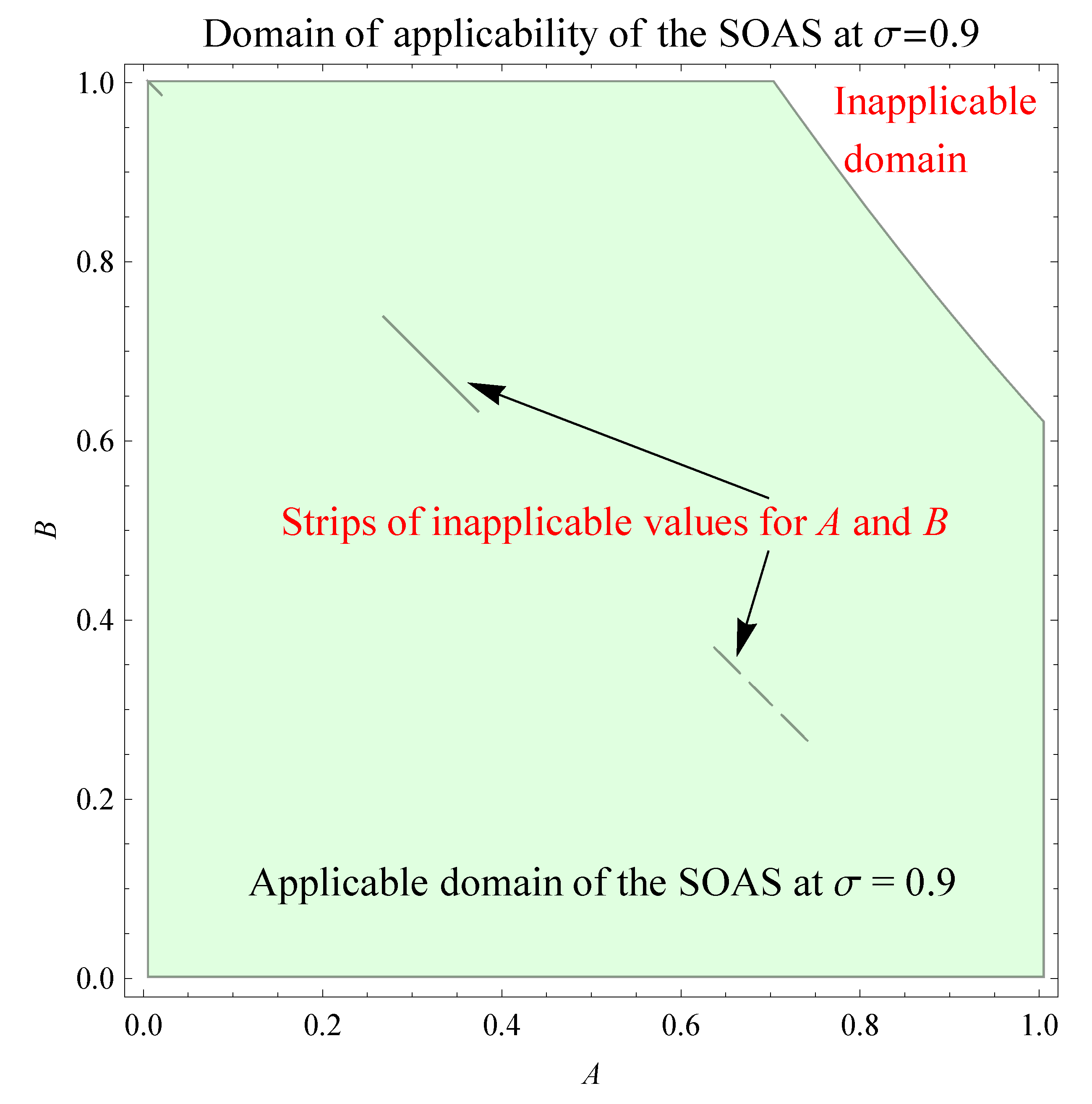
3.2. Second-Order Approximate Solution (SOAS)

Extracting the second-order approximation from the expansion of e σ R and substituting it into Equation (12), we obtain
R ( τ ) = c + 1 ( 1 + c σ ) R ( τ ) + c σ 2 2 R 2 .
Applying ICs (8) to Equation (20) provides c as
c = R ( 0 ) + R ( 0 ) 1 1 σ R ( 0 ) + σ 2 2 R 2 ( 0 ) ,
or
c = 2 ( B + A 1 ) 1 + ( 1 σ A ) 2 .
Equation (20) can be written as
R ( τ ) = c σ 2 2 R 2 2 ( 1 + c σ ) c σ 2 R + 2 ( 1 + c ) c σ 2 ,
or
R ( τ ) = c σ 2 2 R 1 + c σ c σ 2 2 + 2 ( 1 + c ) c σ 2 1 + c σ c σ 2 2 ,
i.e.,
R ( τ ) = c σ 2 2 R ( τ ) β 2 ρ 2 ,
where
β = 1 + c σ c σ 2 , ρ 2 = β 2 2 ( 1 + c ) c σ 2 .
Using the separation of the variable method, Equation (25) can be rewritten as
d R ( τ ) R ( τ ) β 2 ρ 2 = c σ 2 2 d τ .
Integrating both sides, we obtain
1 ρ tan h 1 R ( τ ) β ρ + 1 ρ tan h 1 R ( 0 ) β ρ = c σ 2 2 τ .
i.e.,
1 ρ tan h 1 R ( τ ) β ρ + 1 ρ tan h 1 A β ρ = c σ 2 2 τ ,
which can be written as
R ( τ ) = β + ρ tan h tan h 1 A β ρ c ρ σ 2 2 τ .
Expanding the right side of the last equation provides
R ( τ ) = β + ρ A β ρ tan h c ρ σ 2 2 τ ρ ( A β ) tan h c ρ σ 2 2 τ .
It can be seen from this solution that it satisfies IC R ( 0 ) = A . Further, Solution (31) can be verified by direct substitution into Equation (20). In addition, the solution of the infected cases can be evaluated by differentiating R ( τ ) , thus
I ( τ ) = c ρ 2 σ 2 ( A β ) 2 ρ 2 sec h 2 c ρ σ 2 2 τ 2 ρ ( A β ) tan h c ρ σ 2 2 τ 2 .
This expression can be simplified by employing the relation:
c σ 2 2 A β 2 ρ 2 = B ,
which can be obtained from (25) through inserting ICs R ( 0 ) = A and R ( 0 ) = B . Hence, the soultion of the infected cases is provided in the final form:
I ( τ ) = B ρ 2 sec h 2 c ρ σ 2 2 τ ρ ( A β ) tan h c ρ σ 2 2 τ 2 ,
where c is already provided in (22). At first glance of the solution, one can see that it satisfies the IC I ( 0 ) = B . Moreover, it should be noted that the above expressions for R ( τ ) and I ( τ ) are valid when ρ is real.

4. Features and Behaviors

Normally, it is expected that the value of the infected individuals reduces over time, while the number of recovered individuals reaches a certain constant value at a prescribed interval of time, which may be large or short depending on the nature or data of each country. Equation (12) can be used directly to obtain an accurate prediction of the recovered individuals after a relatively or sufficiently large amount of time τ (say). After this time, i.e., τ > τ , no variation is expected in the number of the recovered individuals, i.e., R ( τ ) = 0 for all τ > τ . Mathematically, one can consider R ( τ ) 0 as τ . Accordingly, the number of recovered individuals, τ , denoted by R , can be predicted through solving the transcendental equation:
1 R + c e σ R = 0 ,
where c is already provided in Equation (13) in terms of σ , A, and B. The above transcendental equation can be solved numerically using software. Moreover, approximate values of R can be estimated from the solutions obtained in the previous section. In this regard, FOAS (18) estimates R as
R = lim τ R ( τ ) = B + ( 1 σ ) A σ B + 1 σ .
It must be noted that the value R in the last equation is restricted by
σ ( B 1 ) + 1 1 σ A > 0 ,
so that solution I ( τ ) in (19) of the infected individuals satisfies the condition:
lim τ I ( τ ) = 0 .
The possible ranges of initial values for A and B, provided that Condition (37) is satisfied, are shown in Figure 1 and Figure 2 at σ = 0.9 and σ = 1 , respectively. Figure 1 indicates that FOAS is valid in the entire ranges of A and B when σ = 0.9 . However, Figure 2 reveals that FOAS is valid in certain domains of A and B when σ = 1 .
On the other hand, SOAS determines R as
R = β + ρ lim τ A β ρ tan h c ρ σ 2 2 τ ρ ( A β ) tan h c ρ σ 2 2 τ = β + ρ = 1 + c σ c σ 2 1 + c σ c σ 2 2 2 ( 1 + c ) c σ 2 ,
where c = 2 ( B + A 1 ) 1 + ( 1 σ A ) 2 < 0 for all A and B, such that 0 < A + B < 1 . Note that Expression (39) for R is valid when ρ is real. This requires discussing the domain of applicability for the involved parameters. From Equation (26), we note that ρ is real if the following condition is satisfied:
1 + c σ c σ 2 2 2 ( 1 + c ) c σ 2 > 0 .
Inserting the constant c = 2 ( B + A 1 ) 1 + ( 1 σ A ) 2 into this condition and performing simplifications, then
( 2 σ B + 2 ( 1 σ ) + σ 2 B 2 ) 2 σ 2 ( 1 A B ) 2 1 2 ( A + B ) ( 1 σ A ) 2 σ 2 ( 1 A B ) > 0 .
Figure 3 and Figure 4 depict the applicable and inapplicable domains of A and B for the validity of SOAS at σ = 0.9 and σ = 1 , respectively.
Regarding the accuracy of the current approximate solutions, Table 1 shows several comparisons between FOAS, SOAS, and the numerical solution using MATHEMATICA for the values of R . It can be seen that the values of R via FOAS are close to the numeric ones when 0.1 σ 0.6 . In addition, SOAS provides better estimations for R , as follows. The results in the SOAS column are identical to the numerical results when σ = 0.1 , σ = 0.2 , and σ = 0.3 (which can be viewed as exact answers at these cases of σ ). Moreover, the values of SOAS agree with the numerical results to six decimal places when σ = 0.4 and σ = 0.5 . For σ = 0.6 , SOAS’s value agrees with the numerical result to five decimal places. For σ = 0.7 and σ = 0.8 , the present values agree with the numerical results to four decimal places. For σ = 0.9 and σ = 1 , the current results agree with the numerical ones to three and two decimal places, respectively. It is important to note that if the exact solution of the nonlinear SIR model is not available, the numerical solution is considered as an optimal solution for the purpose of estimating the accuracy of the present results.

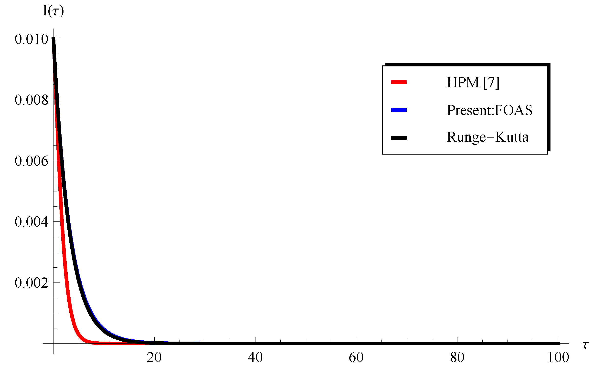
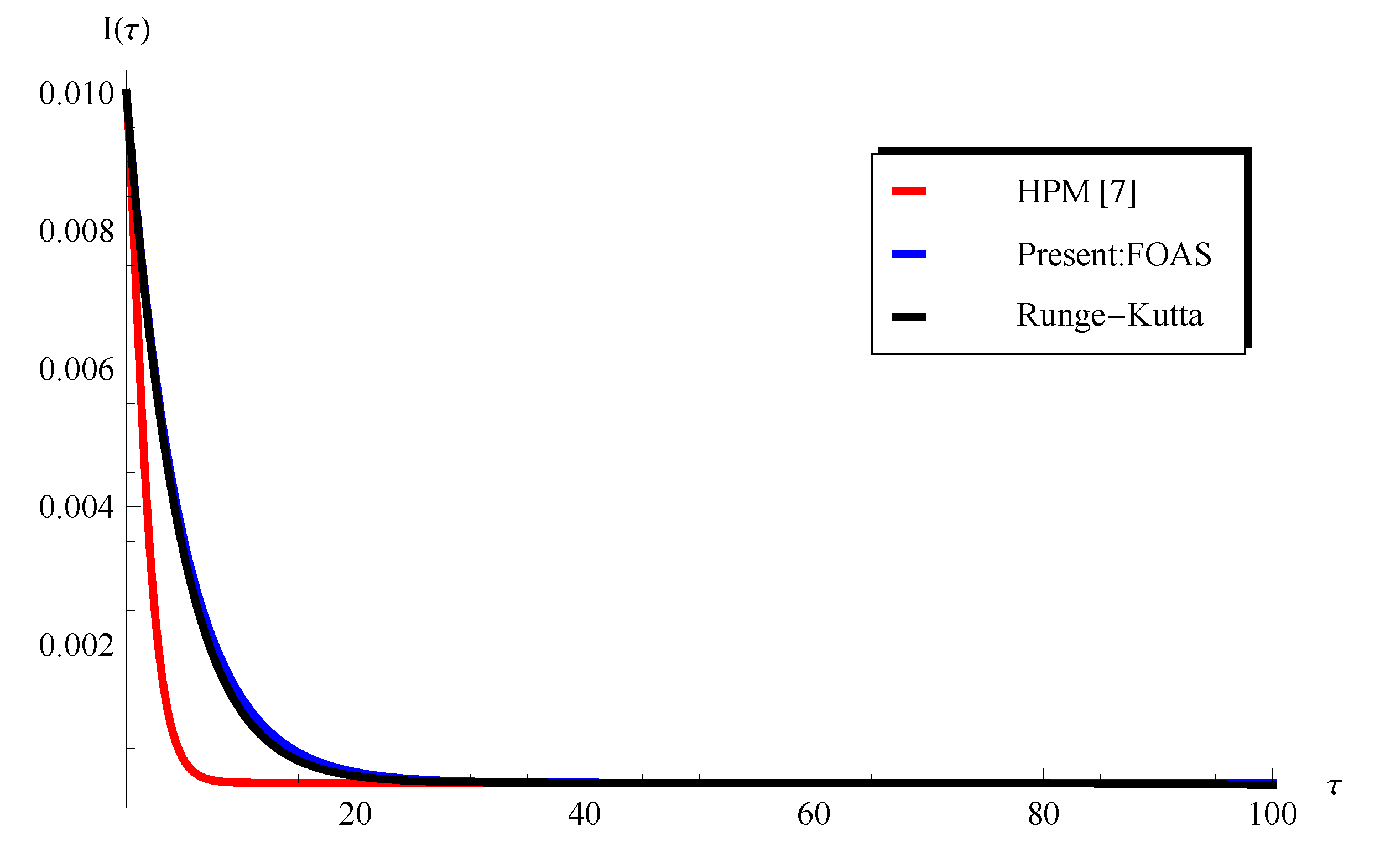
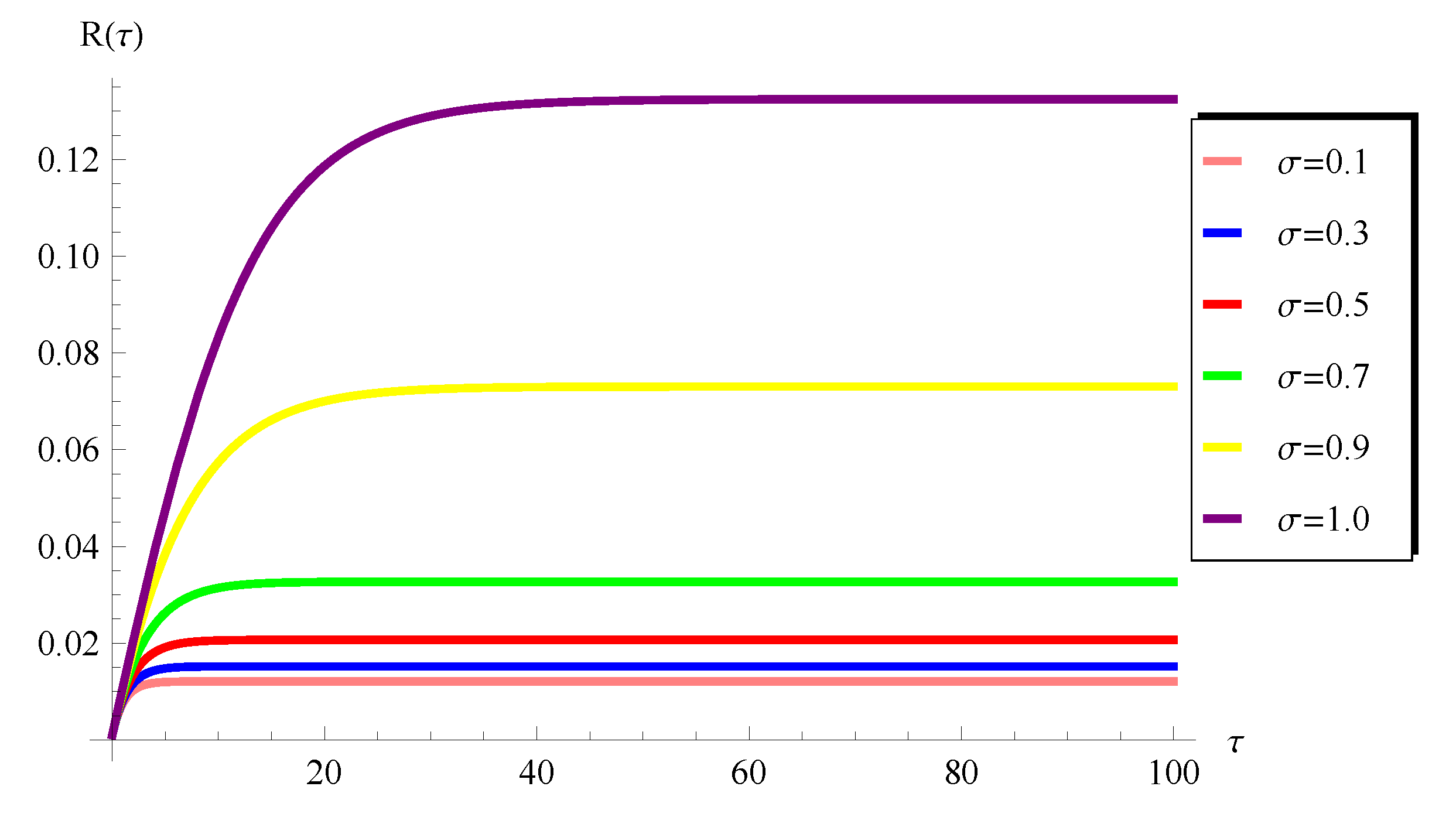
5. Numerical Results and Comparisons with Other Methods

In Ref. [7], the authors applied HPM to systems (1–3) to obtain the following approximate solutions:
R ( t ) = A B e τ + B + σ B B τ e τ e τ 1 2 B e 2 τ + B e τ τ e τ e τ σ B 3 2 B 1 ,
I ( t ) = B e τ + e τ σ B B τ B e τ τ σ B 2 1 2 σ B e τ ( 4 σ B 2 2 σ B + 2 B ) 1 2 σ B e τ [ 4 σ B 2 τ e τ + 6 σ B 2 e τ 2 σ B 2 e 2 τ σ B 2 τ 2 2 σ B 2 τ 2 σ B e τ + 2 σ B τ + 2 σ B τ 2 4 σ B τ e τ + 2 B τ 2 B e τ σ τ 2 ] .
The comparisons between the present FOAS, HPM [7], and numerical solution (Runge–Kutta) are displayed in Figure 5 and Figure 6 for the instantaneous R ( τ ) and I ( τ ) , respectively, for the initial recovered individuals A = 0.001 , initial infected individuals B = 0.01 , and transmission rate σ = 0.5 . The results in these figures show the agreement of the present FOAS with the numerical solution, while HPM [7] deviates; hence, it may need revision. Figure 7 and Figure 8 also indicate the superiority of the present FOAS over HPM [7]; however, the accuracy of FOAS is slightly affected by the small increase in σ ( σ = 0.7 ). Figure 9 and Figure 10 confirm this conclusion that the increase in σ ( σ = 0.8 ) leads to a slight deviation between the present FOAS and the numerical solution; however, the accuracy of FOAS is still better than HPM [7].
Although the FOAS provides accurate solutions in a short range of the transmission rate parameter σ , one can see in Figure 11, Figure 12, Figure 13 and Figure 14 that SOAS is in full agreement with the numerical solution, even for higher values of σ , σ = 0.9 (Figure 11 and Figure 12) and σ = 1 (Figure 13 and Figure 14). This leads to the conclusion that the present SOAS represents an accurate solution for the current COVID-19 model for all values of σ in the range of 0 < σ 1 while HPM [7] does not. Finally, the variations in recovered individuals R ( τ ) and infected individuals I ( τ ) are plotted in Figure 15 and Figure 16 at various values of the transmission rate σ .
As the main point is to compare the solution between different methods, the absolute difference between the present approximations FOAS/SOAS and the Runge–Kutta method is plotted in Figure 17 for the recovered individuals, while the absolute difference between the HPM [7] and Runge-Kutta method is displayed in Figure 18. It can be seen from these two figures that the accuracy of the approximation FOAS is slightly better than HPM [7]. However, the approximation SOAS displayed a better accuracy than HPM [7]. This conclusion can also be confirmed or observed in Figure 19 and Figure 20.

6. Conclusions

In this paper, two different approximate solutions were obtained for a nonlinear COVID-19 model. The obtained approximate solutions were expressed explicitly in terms of exponential and hyperbolic functions. It was shown that the current two approximate solutions displayed many advantages over the HPM solution in the literature [7]. The numerical comparisons between our approximations and the Runge–Kutta method were declared. Moreover, it was proven that the present approximations were more accurate compared with HPM [7], where the Runge–Kutta numerical method was taken as a reference method. Furthermore, the values of the recovered individuals at a sufficiently large time were derived analytically through the two approximations that were obtained. The numerical results reveal that our approach is straightforward and efficient compared with the previous study [7].

Funding

This research received no external funding.

Data Availability Statement

Data are contained within the article.

Conflicts of Interest

The author declares no conflict of interest.

References

  1. Graunt, J. Natural and Political Observations Made Upon the Bills of Mortality; Tho. Roycroft for John Martin, James Allestry, and Tho. Dicas: London, UK, 1662. [Google Scholar]
  2. Bernoulli, D. Essai d’une nouvelle analyse de la mortalite causee par la petite verole et des avantages de l’inoculation pour la prevenir. Mem. Math. Phys. Acad. Roy. Sci. Paris 1760, 1. [Google Scholar]
  3. Kermack, W.O.; McKendrick, A.G. Contribution to the mathematical theory of epidemics. Proc. Roy. Soc. Lond. A 1927, 115, 700–721. [Google Scholar]
  4. Murray, J.D. Mathematical Biology: I. An Introduction; Springer: New York, NY, USA; Berlin/Heidelberg, Germany, 2002. [Google Scholar]
  5. Brauer, F.; van den Driessche, P.; Wu, J. (Eds.) Lecture Notes in Mathematical Epidemiology; Springer: Berlin/Heidelberg, Germany, 2008. [Google Scholar]
  6. De Abajo, J.G. Simple mathematics on COVID-19 expansion. MedRxiv 2020. [Google Scholar]
  7. Gepreel, K.A.; Mohamed, M.S.; Alotaibi, H.; Mahdy, A.M.S. Dynamical Behaviors of Nonlinear Coronavirus (COVID-19) Model with Numerical Studies. Comput. Mater. Contin. 2021, 67, 675–686. [Google Scholar] [CrossRef]
  8. Comunian, A.; Gaburro, R.; Giudici, M. Inversion of a SIR-based model: A critical analysis about the application to COVID-19 epidemic. Phys. D Nonlinear Phenom. 2020, 413, 132674. [Google Scholar] [CrossRef] [PubMed]
  9. Kudryashov, N.A.; Chmykhov, M.A.; Vigdorowitsch, M. Analytical features of the SIR model and their applications to COVID-19. Appl. Math. Model. 2021, 90, 466–473. [Google Scholar] [CrossRef] [PubMed]
  10. Zhou, J.C.; Salahshour, S.; Ahmadian, A.; Senu, N. Modeling the dynamics of COVID-19 using fractal-fractional operator with a case study. Results Phys. 2022, 33, 105103. [Google Scholar] [CrossRef] [PubMed]
  11. Sarkar, K.; Khajanchi, S.; Nieto, J.J. Modeling and forecasting the COVID-19 pandemic in India. Chaos Solitons Fractals 2020, 139, 110049. [Google Scholar] [CrossRef] [PubMed]
  12. Martelloni, G.; Martelloni, G. Modelling the downhill of the SARS-CoV-2 in Italy and a universal forecast of the epidemic in the world. Chaos Solitons Fractals 2020, 139, 110064. [Google Scholar] [CrossRef] [PubMed]
  13. Zhu, W.J.; Shen, S.F. An improved SIR model describing the epidemic dynamics of the COVID-19 in China. Results Phys. 2021, 25, 104289. [Google Scholar] [CrossRef] [PubMed]
  14. Ghosh, K.; Ghosh, A.K. Study of COVID-19 epidemiological evolution in India with a multi-wave SIR model. Nonlinear Dyn. 2022, 109, 47–55. [Google Scholar] [CrossRef] [PubMed]
  15. Ala’raj, M.; Majdalawieh, M.; Nizamuddin, N. Modeling and forecasting of COVID-19 using a hybrid dynamic model based on SEIRD with ARIMA corrections. Infect. Dis. Model. 2021, 6, 98–111. [Google Scholar] [CrossRef] [PubMed]
  16. Margenov, S.; Popivanov, N.; Ugrinova, I.; Hristov, T. Mathematical Modeling and Short-Term Forecasting of the COVID-19 Epidemic in Bulgaria: SEIRS Model with Vaccination. Mathematics 2022, 10, 2570. [Google Scholar] [CrossRef]
  17. Ebaid, A. A reliable aftertreatment for improving the differential transformation method and its application to nonlinear oscillators with fractional nonlinearities. Commun. Nonlin. Sci. Numer. Simul. 2011, 16, 528–536. [Google Scholar] [CrossRef]
  18. Liao, S. Beyond Perturbation: Introduction to the Homotopy Analysis Method; CRC Press: Boca Raton, FL, USA, 2003. [Google Scholar]
  19. Chauhan, A.; Arora, R. Application of homotopy analysis method (HAM) to the non-linear KdV equations Astha Chauhan and Rajan Arora. Commun. Math. 2023, 31, 205–220. [Google Scholar] [CrossRef]
  20. Ayati, Z.; Biazar, J. On the convergence of Homotopy perturbation method. J. Egypt. Math. Soc. 2015, 23, 424–428. [Google Scholar] [CrossRef]
  21. Bayat, M.; Pakar, I.; Bayat, M. Approximate analytical solution of nonlinear systems using homotopy perturbation method. Proc. Inst. Mech. Eng. Part E J. Process Mech. Eng. 2016, 230, 10–17. [Google Scholar] [CrossRef]
  22. Adomian, G. Solving Frontier Problems of Physics: The Decomposition Method; Kluwer Academy: Boston, MA, USA, 1994. [Google Scholar]
Figure 1. Applicable domain for the validity of FOAS at σ = 0.9 .
Axioms 13 00167 g001
Figure 2. Applicable and inapplicable domains for the validity of FOAS at σ = 1 .
Axioms 13 00167 g002
Figure 3. Applicable and inapplicable domains for the validity of SOAS at σ = 0.9 .
Axioms 13 00167 g003
Figure 4. Applicable and inapplicable domains for the validity of SOAS at σ = 1 .
Axioms 13 00167 g004
Figure 5. Comparison between the present FOAS, HPM [7], and numerical solution (Runge–Kutta) at A = 0.001 , B = 0.01 , and σ = 0.5 for R ( τ ) .
Axioms 13 00167 g005
Figure 6. Comparison between the present FOAS, HPM [7], and numerical solution (Runge–Kutta) at A = 0.001 , B = 0.01 , and σ = 0.5 for I ( τ ) .
Axioms 13 00167 g006
Figure 7. Comparison between the present FOAS, HPM [7], and numerical solution (Runge–Kutta) at A = 0.001 , B = 0.01 , and σ = 0.7 for R ( τ ) .
Axioms 13 00167 g007
Figure 8. Comparison between the present FOAS, HPM [7], and numerical solution (Runge–Kutta) at A = 0.001 , B = 0.01 , and σ = 0.7 for I ( τ ) .
Axioms 13 00167 g008
Figure 9. Comparison between the present FOAS, HPM [7], and numerical solution (Runge–Kutta) at A = 0.001 , B = 0.01 , and σ = 0.8 for R ( τ ) .
Axioms 13 00167 g009
Figure 10. Comparison between the present FOAS, HPM [7], and numerical solution (Runge–Kutta) at A = 0.001 , B = 0.01 , and σ = 0.8 for I ( τ ) .
Axioms 13 00167 g010
Figure 11. Comparison between the present SOAS, HPM [7], and numerical solution (Runge–Kutta) at A = 0.001 , B = 0.01 , and σ = 0.9 for R ( τ ) .
Axioms 13 00167 g011
Figure 12. Comparison between the present SOAS, HPM [7], and numerical solution (Runge–Kutta) at A = 0.001 , B = 0.01 , and σ = 0.9 for I ( τ ) .
Axioms 13 00167 g012
Figure 13. Comparison between the present SOAS, HPM [7], and numerical solution (Runge–Kutta) at A = 0.001 , B = 0.01 , and σ = 1 for R ( τ ) .
Axioms 13 00167 g013
Figure 14. Comparison between the present SOAS, HPM [7], and numerical solution (Runge–Kutta) at A = 0.001 , B = 0.01 , and σ = 1 for I ( τ ) .
Axioms 13 00167 g014
Figure 15. Variation in the present SOAS for recovered individuals R ( τ ) at different values of transmission rate σ when A = 0.001 and B = 0.01 .
Axioms 13 00167 g015
Figure 16. Variation in the present SOAS for infected individuals I ( τ ) at different values of transmission rate σ when A = 0.001 and B = 0.01 .
Axioms 13 00167 g016
Figure 17. The absolute error of the present approximations of SOAS and SOAS for recovered individuals R ( τ ) at σ = 0.9 when A = 0.001 and B = 0.01 .
Axioms 13 00167 g017
Figure 18. The absolute error of HPM [7] for recovered individuals R ( τ ) at σ = 0.9 when A = 0.001 and B = 0.01 .
Axioms 13 00167 g018
Figure 19. The absolute error of the present approximations for SOAS and SOAS for infected individuals I ( τ ) at σ = 0.9 when A = 0.001 and B = 0.01 .
Axioms 13 00167 g019
Figure 20. The absolute error of HPM [7] for infected individuals I ( τ ) at σ = 0.9 when A = 0.001 and B = 0.01 .
Axioms 13 00167 g020
Table 1. Comparisons between the approximate values of R (the expected final number of the recovered cases) using the present FOAS and SOAS with the numerical results at different values of contact number σ (transmission rate) for initial infected individuals A = 0.01 and initial recovered individuals B = 0.001 .
σ R (FOAS) R (SOAS) R (Numerical)
0.10.01209770.01209690.0120969
0.20.01346630.01346190.0134619
0.30.01522050.01520590.0152059
0.40.01754970.01750960.0175097
0.50.02079210.02068760.0206879
0.60.02561580.02533480.0253362
0.70.03355050.03270690.0327130
0.80.04903850.04584240.0458764
0.90.09266060.07305300.0733310
1.01.00000000.13245650.1352252
Disclaimer/Publisher’s Note: The statements, opinions and data contained in all publications are solely those of the individual author(s) and contributor(s) and not of MDPI and/or the editor(s). MDPI and/or the editor(s) disclaim responsibility for any injury to people or property resulting from any ideas, methods, instructions or products referred to in the content.

