New Results Achieved for Fractional Differential Equations with Riemann–Liouville Derivatives of Nonlinear Variable Order

Abstract

This paper proposes new existence and uniqueness results for an initial value problem (IVP) of fractional differential equations of nonlinear variable order. Riemann–Liouville-type fractional derivatives are considered in the problem. The new fundamental results achieved in this work are obtained by using the inequalities technique and the fixed point theory. In addition, uniform stability criteria for the solutions are derived. The accomplished results are new and complement the scientific research in the field. A numerical example is composed to show the efficacy and potency of the proposed criteria.

1. Introduction

Differential equations having fractional-order derivatives can be used as models of processes that generally possess boundless memory, which finds an advantage over integer-order differential equations. Indeed, it is known that the heredity properties of processes and materials are better represented by fractional-order derivatives. In addition, fractional-order derivatives and integrals provide more degrees of freedom to the model represented. As such, differential equations in terms of fractional derivatives have been extensively investigated during the last several decades as a technique for precisely describing real systems investigated in numerous fields of science, engineering and medicine [1,2,3,4,5,6,7].

Note that, historically, the first introduced derivatives and integrals in noninteger order were those of the Riemann–Liouville type [8,9]. It is also known that although a Caputo-type derivative of zero is zero, this is not true for the Riemann–Liouville-type fractional derivatives. The last fact leads to some complications in the investigation of fractional differential equations in terms of Riemann–Liouville-type derivatives. However, the excellent suggestions of the physical meaning of initial conditions for Riemann–Liouville fractional differential equations (see, for example, [10]) put these equations into a preferred modeling tool in various fields of science [2,5,11,12,13].

As an extension of the classical fractional differential systems, the type of differential systems with variable order of fractional derivatives has been also studied by numerous researchers using a variety of analytical and numerical methodologies. The fundamental idea that led to such an extension is to replace the constant $\beta$ by a function $\beta (·)$. The basic notion of variable order derivatives has been first proposed by Samko and Ross in [14]. Since then, the investigations of variable order fractional operators in different forms and their applications have attracted more and more attention. For some excellent contributions to the theory of fractional differentiable systems with variable order derivatives we will refer to [15,16,17,18] and the corresponding references. The fractional variable order generalization makes the fractional differential systems in terms of variable order derivatives a more flexible apparatus in modeling various processes and natural phenomena. Hence, there has been an increasing research activity in the theory of such equations [19,20,21,22,23,24], including recently studied applications [25,26,27,28,29] which demonstrated the flexibility of this modeling approach. In fact, fractional differential equations in terms of variable order fractional derivatives have proven to be suitable in modeling numerous phenomena such as anomalous diffusion [28,30], tumor modeling [29], petroleum engineering [31], viscoelastic mechanics [32] and many others [17,25,26,27]. In addition, it has been shown [33] that variable order fractional calculus is a potential candidate to provide an accurate mathematical framework for efficient characterization of complex physical processes and systems.

Even though the substitution of a constant fractional order with a variable fractional order in the fractional derivatives seems simple, there are numerous difficulties in the mathematical investigations of differential systems in terms of variable order fractional derivatives. One of them is related to the absence of the semigroup property [19]. Another mathematical characterization of fractional variable order calculus which is problematic is the circumstance that a fractional derivative of variable order is not necessarily a left-inverse of the corresponding integral [21]. All these complications are reasons for an incomplete evolution of the theory of variable-order fractional differential systems.

Recently, Souid et al. have intensively contributed to this field [34,35,36,37,38,39,40,41,42]. A series of papers is concerned with the questions of the existence and uniqueness of solutions of different classes of differential systems with fractional derivatives of variable order [34,36,37,38,39,40,41,42]. Some of our research papers are devoted to the qualitative analysis of such problems. See, for example, ref. [35] and some of the references therein. In our studies, we apply different techniques such as fixed point theorem, a measure of noncompactness, upper–lower solution methods, piecewise constant functions and some others. The variety of problems investigated includes fractional differential systems with variable order derivatives of Caputo type, Hadamard type and Riemann–Liouville type as well as multiterm fractional boundary value problems of variable order.

In this paper, motivated by the above related works in this regard, we investigate the the following initial value problem (IVP) for fractional differential equations (FDE) with nonlinear variable order (NVO) derivatives of Riemann–Liouville type, defined as follows:

$$\left\{\begin{array}{ccc}{D}_{0^{+}}^{\beta (t,y(t\left)\right)}y\left(t\right)=\psi (t,y\left(t\right)),t\in \mathsf{\Delta }:=(0,M],0<M<\infty ,\hfill & \left(A\right)\hfill & \\ & & \left(\mathrm{IVPFDENVO}\right)\\ y\left(0\right)=0,\hfill & \left(B\right)\hfill & \end{array}\right.$$

where $D_{0^{+}}^{\beta (t,y(t\left)\right)}$ stands for the Riemann–Liouville fractional derivative of the variable order $\beta (t,y(t\left)\right)$, $\psi$ is a given function and $\beta$ satisfies $0<{\beta }_{*}\le \beta (t,y\left(t\right))\le {\beta }^{*}<1$.

Note that, although differential equations with nonlinear variable-order fractional derivatives are already applied as models of numerous problems investigated in science and engineering, the results related to such equations are limited. Hence, the development of the area requires the establishment of new existence and stability results.

The main contributions of our paper are stated as follows:

(1) an IVPFDENVO is defined, which extends some existing problems for fractional-order systems with Riemann–Liouville fractional derivatives of variable order investigated in the literature;

(2) new inequalities are proved for fractional integrals and derivatives of nonlinear variable order;

(3) new criteria for the existence and uniqueness of the solutions to the introduced problem are proposed;

(4) we consider two different Banach spaces of functions to which we apply the inequalities technique and fixed points theorems;

(5) novel uniform stability results are established via an inequalities technique.

The body of the manuscript is organized in the following manner. In Section 2 we present notations, definitions and lemmas that will be necessary to carry out our study. Section 3 is devoted to new existence results for solutions of the IVPFDENVO. A Banach-type fixed point theorem is applied to two different spaces of functions. In Section 4, uniform stability criteria are derived. Section 5 represents numerical applications and simulations. Finally, conclusion remarks are presented in Section 6.

2. Preliminaries

Some preliminary results will be presented in this section together with the related notations and definitions.

We consider the Banach space of all real-valued continuous functions $x:\mathsf{\Delta }\to \mathbb{R}$, $\mathbb{R}=(-\infty ,\infty )$, with the norm

$${\parallel x\parallel }_{\infty }=sup\left\{\left|x\right(t\left)\right|:t\in \mathsf{\Delta }\right\}$$

which we will denoted by $C(\mathsf{\Delta },\mathbb{R})$.

The Banach space of all functions $x:\mathsf{\Delta }\to \mathbb{R}$ such that

$$0<\gamma <1\mathrm{and}{t}^{\gamma }x\left(t\right)\in C(\mathsf{\Delta },\mathbb{R})$$

with the norm

$${\parallel x\parallel }_{\gamma }=sup\{t^{\gamma }\left|x\left(t\right)\right|:t\in \mathsf{\Delta }\}$$

will be denoted by the symbol $C_{\gamma }(\mathsf{\Delta },\mathbb{R})$.

The symbol $L^p(\mathsf{\Delta },\mathbb{R})$ represents the Banach space of all functions $x:\mathsf{\Delta }\to \mathbb{R}$ which are Lebesgue measurable such that

$$p\ge 1\mathrm{and}{\int }_0^M{\left|x\left(s\right)\right|}^{p}ds<\infty$$

with the norm

$${\parallel x\parallel }_p=:{\left({\int }_0^M{\left|x\left(s\right)\right|}^{p}ds\right)}^{{\displaystyle \frac{1}{p}}}.$$

Remark 1.

The following observations are made to make our study easy in the sequel:

(1)

if $0<M\le 1$ then $M^{\beta (s,y(s\left)\right)-1}\le M^{{\beta }_{*}-1}$.

(2)

if $1<M$ then $M^{\beta (s,y(s\left)\right)-1}\le 1$.

Set

$${\mathsf{\Lambda }}^{*}=max\{1,M^{{\beta }_{*}-1}\}.$$

(1)

(3)

The function $\mathsf{\Gamma }\left(\beta \right(t,f\left(t\right)\left)\right)$ is continuous as a composition of two continuous functions, hence we can set:

$$M_f=\underset{t\in [0,M]}{max}\left|\frac{1}{\mathsf{\Gamma }\left(\beta \right(t,f\left(t\right))}\right|.$$

(2)

Let us consider two continuous functions $\beta :\mathsf{\Delta }\times \mathbb{R}\to (0,{\beta }^{*}]$ and $\alpha :\mathsf{\Delta }\times \mathbb{R}\to (0,{\alpha }^{*}]$. Let $f\left(t\right)\in C(\mathsf{\Delta },\mathbb{R})$.

Definition 1

([14,16,18]). The left Riemann–Liouville type integral of fractional variable order β, $\beta =\beta (t,f(t\left)\right)$ for $f\left(t\right)$ is

$$I_{a_1^{+}}^{\beta (t,f(t\left)\right)}f\left(t\right)={\int }_{a_1}^t\frac{{(t-s)}^{\beta (s,f(s\left)\right)-1}}{\mathsf{\Gamma }\left(\beta \right(s,f\left(s\right)\left)\right)}f\left(s\right)ds,t>a_1,$$

(3)

where $\mathsf{\Gamma }(·)$ denotes the Gamma function and $a_1\in \mathsf{\Delta }$.

If $\beta (t,y(t\left)\right)$ is a constant β, then (3) will be reduced to the standard Riemann–Liouville fractional integral of a constant fractional order given by [2,3,5]

$$I_{a_1^{+}}^{\beta }f\left(t\right)=\frac{1}{\mathsf{\Gamma }\left(\beta \right)}{\int }_{{\beta }_{*}}^t{(t-s)}^{\beta -1}f\left(s\right)ds,t>a_1.$$

(4)

Definition 2

([14,16,18]). The left Riemann–Liouville type derivative of fractional variable order α, $\alpha =\alpha (t,f(t\left)\right)$ for a function $f\left(t\right)$ is given by

$$D_{a_1^{+}}^{\alpha (t,f(t\left)\right)}f\left(t\right)=\frac{d}{dt}{I}_{a_1^{+}}^{1-\alpha (t,f(t\left)\right)}f\left(t\right)=\frac{d}{dt}{\int }_{a_1}^t\frac{{(t-s)}^{-\alpha (s,f(s\left)\right)}}{\mathsf{\Gamma }(1-\alpha (s,f\left(s\right)\left)\right)}f\left(s\right)ds,t>a_1.$$

(5)

If $\alpha (t,y(t\left)\right)$ is a constant α, then (5) will become

$$D_{a_1^{+}}^{\alpha }f\left(t\right)=\frac{d}{dt}{I}_{a_1^{+}}^{1-\alpha }f\left(t\right)=\frac{d}{dt}{\int }_{a_1}^t\frac{{(t-s)}^{-\alpha }}{\mathsf{\Gamma }(1-\alpha )}f\left(s\right)ds,t>a_1,$$

(6)

which represents the Riemann–Liouville derivative of a constant fractional order α [2,3,5].

For more characteristics of the integrals and derivatives of fractional constant orders we refer to [2,3,5], and about the integrals and derivatives of fractional variable orders, see [14,16,19].

Remark 2.

It is observed that the semigroup property is not always fulfilled for general functions $\beta (t,y(t\left)\right)$, $\alpha (t,y(t\left)\right)$; i.e., it is possible

$$I_{a_1^{+}}^{\beta (t,f(t\left)\right)}{I}_{a_1^{+}}^{\alpha (t,f(t\left)\right)}f\left(t\right)\ne I_{a_1^{+}}^{\beta (t,f(t\left)\right)+\alpha (t,f(t\left)\right)}f\left(t\right).$$

For more details, see [23,38,43].

We will present some specifications of the fractional integrals of the Riemann–Liouville type of constant orders which will be used in the coming lemmas.

Lemma 1

([3]). If $\gamma \in \mathbb{R}$, then the Riemann–Liouville type integral of fractional constant order is bounded in $C_{\gamma }(\mathsf{\Delta },\mathbb{R})$ and we have for $f\in C_{\gamma }(\mathsf{\Delta },\mathbb{R})$

$$\parallel I_{0^{+}}^{\alpha }{f\parallel }_{\gamma }\le {\displaystyle \frac{M^{\alpha }\mathsf{\Gamma }(1-\gamma )}{\mathsf{\Gamma }(1+\alpha -\gamma )}}{\parallel f\parallel }_{\gamma },\alpha >0$$

(7)

Lemma 2

([3]). If $\gamma \in \mathbb{R}$, then the Riemann–Liouville type fractional integral is bounded in $L^p(\mathsf{\Delta },\mathbb{R})$ and we have for $f\in L^p(\mathsf{\Delta },\mathbb{R})$

$$\parallel I_{0^{+}}^{\alpha }{f\parallel }_p\le {\displaystyle \frac{M^{\alpha }}{\alpha \mathsf{\Gamma }\left(\alpha \right)}}{\parallel f\parallel }_p,\alpha >0.$$

(8)

On the base of Lemmas 1 and 2, we will prove similar inequalities for fractional integrals of nonlinear variable order of Riemann–Liouville type.

Lemma 3.

If $\beta :\mathsf{\Delta }\times \mathbb{R}\to (0,1]$ is a continuous function, such that $0<{\beta }_{*}\le \beta (t,f\left(t\right))\le {\beta }^{*}<1$, then $I_{0^{+}}^{\beta (t,y(t\left)\right)}f\left(t\right)\in C_{\gamma }(\mathsf{\Delta },\mathbb{R})$ for $f\in C_{\gamma }(\mathsf{\Delta },\mathbb{R})$. Moreover, we have:

(i)

$$\parallel I_{0^{+}}^{\beta (t,f(t\left)\right)}{f\parallel }_{\gamma }\le {\displaystyle \frac{M\mathsf{\Gamma }(1-\gamma )\mathsf{\Gamma }\left({\beta }_{*}\right)M_f{\mathsf{\Lambda }}^{*}}{\mathsf{\Gamma }(1+{\beta }_{*}-\gamma )}}{\parallel f\parallel }_{\gamma }.$$

(9)

(ii) For $f,g\in C_{\gamma }(\mathsf{\Delta },\mathbb{R})$, we have

$$\parallel I_{0^{+}}^{\beta (t,f(t\left)\right)}f-I_{0^{+}}^{\beta (t,g(t\left)\right)}{g\parallel }_{\gamma }\le \frac{4MB\mathsf{\Gamma }\left({\beta }_{*}\right){\mathsf{\Lambda }}^{*}\mathsf{\Gamma }(1-\gamma )}{\mathsf{\Gamma }(1+{\beta }_{*}-\gamma )}{\parallel f-g\parallel }_{\gamma },$$

(10)

where $B=max\left\{M_f,M_g\right\}$, ${\mathsf{\Lambda }}^{*}$ is defined by Equation (1) and $M_f$ and $M_g$ are defined by Equation (2).

Proof. 

(i) Let $f\in C_{\gamma }(\mathsf{\Delta },\mathbb{R})$. From Equation (3) we have

$$\begin{array}{cc}{\displaystyle |I_{0^{+}}^{\beta (t,f(t\left)\right)}f\left(t\right)|}\hfill & {\displaystyle \le M_f{\int }_0^t{(t-s)}^{\beta (s,f(s\left)\right)-1}\left|f\left(s\right)\right|ds}\hfill \\ \\ \hfill & {\displaystyle \le M_f{\int }_0^t{M}^{\beta (s,f(s\left)\right)-1}{\left({\displaystyle \frac{t-s}{M}}\right)}^{\beta (s,f(s\left)\right)-1}\left|f\left(s\right)\right|ds}\hfill \\ \\ \hfill & {\displaystyle \le \frac{M_f{\mathsf{\Lambda }}^{*}}{M^{{\beta }_{*}-1}}{\int }_0^t{(t-s)}^{{\beta }_{*}-1}\left|f\left(s\right)\right|ds}\hfill \\ \\ \hfill & {\displaystyle \le \frac{\mathsf{\Gamma }\left({\beta }_{*}\right)M_f{\mathsf{\Lambda }}^{*}}{M^{{\beta }_{*}-1}}{I}_{0^{+}}^{{\beta }_{*}}\left|f\left(t\right)\right|.}\hfill \end{array}$$

(11)

The above estimate implies

$$\parallel I_{0^{+}}^{\beta (t,f(t\left)\right)}{f\parallel }_{\gamma }\le {\displaystyle \frac{\mathsf{\Gamma }\left({\beta }_{*}\right)M_f{\mathsf{\Lambda }}^{*}}{M^{{\beta }_{*}-1}}}\parallel I_{0^{+}}^{{\beta }_{*}}{\left|f\right|\parallel }_{\gamma }.$$

We apply (7) to obtain

$$\parallel I_{0^{+}}^{\beta (t,f(t\left)\right)}{f\parallel }_{\gamma }\le {\displaystyle \frac{M\mathsf{\Gamma }(1-\gamma )\mathsf{\Gamma }\left({\beta }_{*}\right)M_f{\mathsf{\Lambda }}^{*}}{\mathsf{\Gamma }(1+{\beta }_{*}-\gamma )}}{\parallel f\parallel }_{\gamma }.$$

(ii) For $f,g\in C_{\gamma }(\mathsf{\Delta },\mathbb{R})$, we have

$$\begin{array}{cc}\left|I_{0^{+}}^{\beta (t,f(t\left)\right)}f\left(t\right)-I_{0^{+}}^{\beta (t,g(t\left)\right)}g\left(t\right)\right|\hfill & {\displaystyle =\left|{\int }_0^t\frac{{(t-s)}^{\beta (s,f(s\left)\right)-1}}{\mathsf{\Gamma }\left(\beta \right(s,f\left(s\right)\left)\right)}f\left(s\right)ds-\frac{{(t-s)}^{\beta (s,g(s\left)\right)-1}}{\mathsf{\Gamma }\left(\beta \right(s,g\left(s\right)\left)\right)}g\left(s\right)ds\right|}\hfill \\ \\ \hfill & {\displaystyle \le 2B{\mathsf{\Lambda }}^{*}{\int }_0^t\left({\left(\frac{t-s}{M}\right)}^{\beta (s,f(s\left)\right)-1}+{\left(\frac{t-s}{M}\right)}^{\beta (s,g(s\left)\right)-1}\right)}\hfill \\ \\ \hfill & \times \left|f\right(s)-g(s\left)\right|ds\hfill \\ \\ \hfill & {\displaystyle \le \frac{4B{\mathsf{\Lambda }}^{*}}{M^{{\beta }_{*}-1}}{\int }_0^t\left({(t-s)}^{{\beta }_{*}-1}\right)|f\left(s\right)-g\left(s\right)|ds}\hfill \\ \\ \hfill & {\displaystyle \le \frac{4B\mathsf{\Gamma }\left({\beta }_{*}\right){\mathsf{\Lambda }}^{*}}{M^{{\beta }_{*}-1}}{I}_{0^{+}}^{{\beta }_{*}}|f\left(s\right)-g\left(s\right)|,}\hfill \end{array}$$

(12)

which, after the application of (7), implies

$$\parallel I_{0^{+}}^{\beta (t,f(t\left)\right)}f-I_{0^{+}}^{\beta (t,g(t\left)\right)}{g\parallel }_{\gamma }\le \frac{4MB\mathsf{\Gamma }\left({\beta }_{*}\right){\mathsf{\Lambda }}^{*}\mathsf{\Gamma }(1-\gamma )}{\mathsf{\Gamma }(1+{\beta }_{*}-\gamma )}{\parallel f-g\parallel }_{\gamma }.$$

□

Lemma 4.

If $\beta :\mathsf{\Delta }\times \mathbb{R}\to (0,1]$ is a continuous function, such that $0<{\beta }_{*}\le \beta (t,f\left(t\right))\le {\beta }^{*}<1$, then $I_{0^{+}}^{\beta (t,f(t\left)\right)}f\left(t\right)\in L^p(\mathsf{\Delta },\mathbb{R})$ for $f\in L^p(\mathsf{\Delta },\mathbb{R})$. Moreover, we have:

(i)

$$\parallel I_{0^{+}}^{\beta (t,f(t\left)\right)}{f\parallel }_p\le \frac{M{M}_f{\mathsf{\Lambda }}^{*}}{{\beta }_{*}}{\parallel f\parallel }_p.$$

(13)

(ii) For $f,g\in L^p(\mathsf{\Delta },\mathbb{R})$ we have

$$\parallel I_{0^{+}}^{\beta (t,f(t\left)\right)}f-I_{0^{+}}^{\beta (t,g(t\left)\right)}{g\parallel }_p\le \frac{4MB{\mathsf{\Lambda }}^{*}}{{\beta }_{*}}{\parallel f-g\parallel }_p.$$

(14)

Proof. 

(i) Using (9), we obtain

$$\parallel I_{0^{+}}^{\beta (t,f(t\left)\right)}{f\parallel }_p\le {\displaystyle \frac{\mathsf{\Gamma }\left({\beta }_{*}\right)M_f{\mathsf{\Lambda }}^{*}}{M^{{\beta }_{*}-1}}}\parallel I_{0^{+}}^{{\beta }_{*}}{\left|f\right|\parallel }_p.$$

Now, we apply Equation (8) to obtain

$$\parallel I_{0^{+}}^{\beta (t,f(t\left)\right)}{f\parallel }_p\le \frac{M{M}_f{\mathsf{\Lambda }}^{*}}{{\beta }_{*}}{\parallel f\parallel }_p.$$

(ii) We combine Equation (12) with the Hölder’s inequality to obtain

$$\begin{array}{cc}|I_{0^{+}}^{\beta (t,f(t\left)\right)}f\left(t\right)-I_{0^{+}}^{\beta (t,g(t\left)\right)}{g\left(t\right)|}^p\hfill & {\displaystyle \le {\left[\frac{4B\mathsf{\Gamma }\left({\beta }_{*}\right){\mathsf{\Lambda }}^{*}}{M^{{\beta }_{*}-1}}{I}_{0^{+}}^{{\beta }_{*}}|f\left(s\right)-g\left(s\right)|\right]}^p}\hfill \\ \\ \hfill & {\displaystyle \le {\left[\frac{4B\mathsf{\Gamma }\left({\beta }_{*}\right){\mathsf{\Lambda }}^{*}}{M^{{\beta }_{*}-1}}\right]}^p{\left(I_{0^{+}}^{{\beta }_{*}}|f\left(s\right)-g\left(s\right)|\right)}^p.}\hfill \end{array}$$

(15)

Integrating both sides of (15) on $[0,M]$ and take $\frac{1}{p}$-root on both sides, we obtain

$$\parallel I_{0^{+}}^{\beta (t,f(t\left)\right)}f-I_{0^{+}}^{\beta (t,g(t\left)\right)}{g\parallel }_p\le \frac{4MB{\mathsf{\Lambda }}^{*}}{{\beta }_{*}}{\parallel f-g\parallel }_p.$$

The proof of (12) is completed. □

The following lemma will also be useful.

Lemma 5

([44]). Let Θ be a nonempty, bounded Banach space and $F:\mathsf{\Theta }⟶\mathsf{\Theta }$ be a mapping such that for some $n\in \mathbb{N}$, $F^n$ is a contraction, where $F^n=F\circ F\circ \dots \circ F$ n times. Then F has a unique fixed point in Θ.

3. Achieved Existence Results

Definition 3.

A function $y\in C_{\gamma }(\mathsf{\Delta },\mathbb{R})$ or $y\in L^p(\mathsf{\Delta },\mathbb{R})$ is said to be a solution for (IVPFDENVO) if and only if it verifies (IVPFDENVO(A)) and (IVPFDENVO(B)), simultaneously.

In order to present our new existence results in the Banach spaces $C_{\gamma }(\mathsf{\Delta },\mathbb{R})$ and $L^p(\mathsf{\Delta },\mathbb{R})$, we will analyze an equivalent integral form of the IVPFDENVO(A).

Lemma 6.

Let y be an element of $C_{\gamma }(\mathsf{\Delta },\mathbb{R})$ or $L^p(\mathsf{\Delta },\mathbb{R})$. Then, equation (IVPFDENVO(A)) is equivalent to

$$I_{0^{+}}^{1-\beta (t,y(t\left)\right)}y\left(t\right)={\int }_0^t\frac{{(t-s)}^{-\beta (s,y(s\left)\right)}}{\mathsf{\Gamma }(1-\beta (s,y\left(s\right)\left)\right)}y\left(s\right)ds={\int }_0^t\psi (s,y\left(s\right))ds,t\in \mathsf{\Delta }.$$

(16)

Proof. 

Let $y\in C_{\gamma }(\mathsf{\Delta },\mathbb{R})$ or $y\in L^p(\mathsf{\Delta },\mathbb{R})$. Then, for equation (IVPFDENVO(A)) we have the following representation

$$D_{0^{+}}^{\beta (t,y(t\left)\right)}y\left(t\right)=\frac{d}{dt}{\int }_0^t\frac{{(t-s)}^{-\beta (s,y(s\left)\right)}}{\mathsf{\Gamma }(1-\beta (s,y\left(s\right)\left)\right)}y\left(s\right)ds=\psi (t,y\left(t\right)).$$

(17)

Then, both sides of (17) can be integrated from $[0,t]$, to obtain

$${\int }_0^t\frac{{(t-s)}^{-\beta (s,y(s\left)\right)}}{\mathsf{\Gamma }(1-\beta (s,y\left(s\right)\left)\right)}y\left(s\right)ds=c_0+{\int }_0^t\psi (s,y\left(s\right))ds.$$

(18)

Evaluating (18) at $t=0$ gives us $c_0=0$.

Conversely, differentiating both sides of (16) to reach

$$\frac{d}{dt}{\int }_0^t\frac{{(t-s)}^{-\beta (s,y(s\left)\right)}}{\mathsf{\Gamma }(1-\beta (s,y\left(s\right)\left)\right)}y\left(s\right)ds=\psi (t,y\left(t\right)),$$

(19)

from which we obtain (IVPFDENVO(A)).

The proof is concluded. □

The following assumptions will be essential in our analysis.

(A1)

The function $\beta :\mathsf{\Delta }\times \mathbb{R}\to (0,{\beta }^{*}]$ is continuous on its domain.

(A2)

The function $\psi :\mathsf{\Delta }\times \mathbb{R}\to \mathbb{R}$ is a continuous function with respect to its first variable and satisfies:

$$\left|\psi (s,{\chi }_1)-\psi (s,{\chi }_2)\right|\le k|{\chi }_1-{\chi }_2|,\forall {\chi }_1,{\chi }_2\in \mathbb{R}$$

for $t\in \mathsf{\Delta }$ and $k>0$.

3.1. Existence Result in $C_{\gamma }(\mathsf{\Delta },\mathbb{R})$

The first obtained result is based on Lemma 5.

Theorem 1.

Assume that (A1) and (A2) are satisfied. Then the (IVPFDENVO) has a unique solution in $C_{1-{\beta }^{*}}(\mathsf{\Delta },\mathbb{R})$.

Proof. 

Let us consider $\gamma =1-{\beta }^{*}$ and the set of elements $\mathsf{\Theta }$ in the space $C_{\gamma }(\mathsf{\Delta },\mathbb{R})$ such that $y\left(0\right)=0$. Define the following operator

$$\mathsf{\Pi }:\mathsf{\Theta }\to \mathsf{\Theta },$$

where

$$\left(\mathsf{\Pi }y\right)\left(t\right)=y\left(t\right)+I_{0^{+}}^{1-\beta (t,y(t\left)\right)}y\left(t\right)-{\int }_0^t\psi (s,y\left(s\right))ds.$$

(20)

First, for two $x,y:\mathsf{\Delta }\to \mathbb{R}$ using (A2), we have

$$\left|{\int }_0^t\left[\psi (s,x(s\left)\right)-\psi (s,y(s\left)\right)\right]ds\right|\le k{t}^{-\gamma }\left|\right|y-{x\left|\right|}_{\gamma }.$$

Then, from (18) we can obtain the following estimation

$$\begin{array}{cc}\left|\right(\mathsf{\Pi }x\left)\right(t)-(\mathsf{\Pi }y\left)\right(t\left)\right|\hfill & {\displaystyle \le |y\left(t\right)-x\left(t\right)|+|I_{0^{+}}^{1-\beta (t,x(t\left)\right)}x\left(t\right)-I_{0^{+}}^{1-\beta (t,y(t\left)\right)}y\left(t\right)|}\hfill \\ \\ \hfill & {\displaystyle +\left|{\int }_0^t\left[\psi (s,x(s\left)\right)-\psi (s,y(s\left)\right)\right]ds\right|}\hfill \\ \\ \hfill & {\displaystyle \le t^{-\gamma }\left|\right|y-{x\left|\right|}_{\gamma }+|I_{0^{+}}^{1-\beta (t,x(t\left)\right)}x\left(t\right)-I_{0^{+}}^{1-\beta (t,y(t\left)\right)}y\left(t\right)|+k{t}^{-\gamma }\left|\right|y-{x\left|\right|}_{\gamma }.}\hfill \end{array}$$

(21)

We multiply both sides of Equation (21) with $t^{\gamma }$ and take the sup of both sides to obtain

$$\left|\right|\mathsf{\Pi }x-{\mathsf{\Pi }y\left|\right|}_{\gamma }\le \left|\right|y-{x\left|\right|}_{\gamma }+\left|\right|I_{0^{+}}^{1-\beta (t,x(t)}x-I_{0^{+}}^{1-\beta (t,y(t)}{y\left|\right|}_{\gamma }+k\left|\right|y-{x\left|\right|}_{\gamma }.$$

Using Equation (10) we obtain

$$\left|\right|\mathsf{\Pi }x-{\mathsf{\Pi }y\left|\right|}_{\gamma }\le \left|\right|y-{x\left|\right|}_{\gamma }+\frac{4MB\mathsf{\Gamma }{\left({\beta }^{*}\right)}^2{\mathsf{\Lambda }}^{*}}{\mathsf{\Gamma }\left(2{\beta }^{*}\right)}{\parallel y-x\parallel }_{\gamma }+k\left|\right|y-{x\left|\right|}_{\gamma }.$$

If we set ${\displaystyle \zeta =\left(1+\frac{4MB\mathsf{\Gamma }{\left({\beta }^{*}\right)}^2{\mathsf{\Lambda }}^{*}}{\mathsf{\Gamma }\left(2{\beta }^{*}\right)}+k\right),}$ then we have

$$\left|\right|\mathsf{\Pi }x-{\mathsf{\Pi }y\left|\right|}_{\gamma }\le \zeta \left|\right|y-{x\left|\right|}_{\gamma }.$$

By induction, it is trivial to prove that

$$\left|\right|{\mathsf{\Pi }}^{n}x-{\mathsf{\Pi }}^n{y\left|\right|}_{\gamma }\le \frac{{\zeta }^n}{n!}\left|\right|y-{x\left|\right|}_{\gamma },$$

where ${\mathsf{\Pi }}^n=\mathsf{\Pi }\circ \mathsf{\Pi }\circ \dots \circ \mathsf{\Pi }$ n times.

Since $\frac{{\zeta }^n}{n!}$ is the general term of the convergent exponential series $e^{\zeta }$, it approaches zero as n approaches infinity, and so for n sufficiently large we have

$$\frac{{\zeta }^n}{n!}<1.$$

Lemma 5 asserts that the operator $\mathsf{\Pi }$ has a unique fixed point in $\mathsf{\Theta }$.

This implies that

$$I_{0^{+}}^{1-\beta (t,y(t\left)\right)}y\left(t\right)={\int }_0^t\psi (s,y\left(s\right))ds$$

(22)

with $y\left(0\right)=0$

Finally, from Lemma 6, we obtain

$$D_{0^{+}}^{\beta (t,y(t\left)\right)}y\left(t\right)=\psi (t,y\left(t\right))withy\left(0\right)=0.$$

(23)

This concludes our proof. □

3.2. Existence Result in $L^p(\mathsf{\Delta },\mathbb{R})$

Theorem 2.

Under the assumptions (A1) and (A2), the (IVPFDENVO) has a unique solution in the Banach space $L^p(\mathsf{\Delta },\mathbb{R})$.

Proof. 

We consider the set $\mathsf{\Theta }$ as an element in $L^p(\mathsf{\Delta },\mathbb{R})$ such that $y\left(0\right)=0$, and the operator

$$\mathsf{\Pi }:\mathsf{\Theta }\to \mathsf{\Theta },$$

where

$${\displaystyle \left(\mathsf{\Pi }y\right)\left(t\right)=y\left(t\right)+I_{0^{+}}^{1-\beta (t,y(t\left)\right)}y\left(t\right)-{\int }_0^t\psi (s,y\left(s\right))ds.}$$

Then, we have from (A2) that for $x,y:\mathsf{\Delta }\to \mathbb{R}$,

$$\left|{\int }_0^t\psi (s,x\left(s\right))-\psi (s,y\left(s\right))ds\right|\le k{M}^{1/p}\left|\right|y-{x\left|\right|}_p$$

and

$$\begin{array}{cc}{|\left(\mathsf{\Pi }x\right)\left(t\right)-\left(\mathsf{\Pi }y\right)\left(t\right)|}^p\hfill & {\displaystyle \le 2^p\left({|y\left(t\right)-x\left(t\right)|}^p+|I_{0^{+}}^{1-\beta (t,x(t\left)\right)}x\left(t\right)-I_{0^{+}}^{1-\beta (t,y(t\left)\right)}y\left(t\right){\left)\right|}^p\right.}\hfill \\ \\ \hfill & {\displaystyle +\left.{\left|{\int }_0^t\psi (s,x\left(s\right))-\psi (s,y\left(s\right))ds\right|}^p\right)}\hfill \\ \\ \hfill & {\displaystyle \le 2^p\left({|y\left(t\right)-x\left(t\right)|}^p+{|I_{0^{+}}^{1-\beta (t,x(t\left)\right)}x\left(t\right)-I_{0^{+}}^{1-\beta (t,y(t\left)\right)}y\left(t\right)|}^p\right.}\hfill \\ \\ \hfill & +\left.k^{p}M\left|\right|y-{x\left|\right|}_p^p\right).\hfill \end{array}$$

(24)

Integrating Equation (24) on $[0,M]$, we obtain

$$\left|\right|\mathsf{\Pi }x-{\mathsf{\Pi }y\left|\right|}_p^p\le 2^p\left(\left|\right|y-{x\left|\right|}_p^p+\left|\right|I_{0^{+}}^{1-\beta (t,x(t\left)\right)}x-I_{0^{+}}^{1-\beta (t,y(t\left)\right)}{y\left|\right|}_p^p+k^p{M}^2\left|\right|y-{x\left|\right|}_p^p\right).$$

Using Equation (14) from Lemma 4, we obtain

$$\begin{array}{cc}\left|\right|\mathsf{\Pi }x-{\mathsf{\Pi }y\left|\right|}_p^p\hfill & {\displaystyle \le 2^p\left(\right||y-{x\left|\right|}_p^p+{\left[\frac{4MB{\mathsf{\Lambda }}^{*}}{1-{\beta }^{*}}\right]}^p{\parallel y-x\parallel }_p^p+k^p{M}^2\left|\right|y-{x\left|\right|}_p^p)}\hfill \\ \\ & {\displaystyle \le 2^p\left(1+{\left[\frac{4MB{\mathsf{\Lambda }}^{*}}{1-{\beta }^{*}}\right]}^p+k^p{M}^2\right)\left|\right|y-{x\left|\right|}_p^p.}\hfill \end{array}$$

If we denote $\zeta =2{\left(1+{\left[\frac{4MB{\mathsf{\Lambda }}^{*}}{1-{\beta }^{*}}\right]}^p+k^p{M}^2\right)}^{\frac{1}{p}},$ then the assertion of the theorem can be proved analogously to the final part of the proof of Theorem 1.

This concludes our proof. □

Remark 3.

Since the operators involved in the description of fractional differential equations of variable nonlinear fractional order have complex properties, the research results in this direction are still limited [23,34,36,37,38,39,40,41,42,43]. With the proposed new criteria in Theorems 1 and 2, we complement and extend the existence of theoretical results for such initial value problems. The delivered results are obtained by using fixed point theory and are presented in two different Banach spaces.

Remark 4.

The criteria presented in this section are also extensions and generalizations of some announced results that are considered initial value problems for fractional constant-order differential equations to the variable order case [45,46,47,48]. In fact, the consideration of nonlinear variable orders leads to the definition of more complex and generalized problems that can be used in the applications.

Remark 5.

Different from the existing results for differential systems with fractional derivatives of variable order, in this study, we consider fractional derivatives of Riemann–Liouville types of order $\beta :\mathsf{\Delta }\times \mathbb{R}\to (0,1]$. Instead of the approaches introduced in [23,43], such as piecewise continuous functions and the Picard scheme, we apply the operator approach and a Banach-type fixed point theorem, which we consider as more appropriate for the considered problem from the applied perspective. The proposed strategy can be applied to similar problems considering delays and impulsive factors, which can motivate future research.

4. Uniform Stability

In this Section, the newly achieved existence and uniqueness results will be applied to derive uniform stability criteria for the solution of the (IVPFDENVO).

Consider a solution $x\left(t\right)$ of the equation IVPFDENVO(A) corresponding to an initial condition $y\left(0\right)=x_0$. Let $\overline{x}\left(t\right)$ be another solution of equation IVPFDENVO(A) corresponding to an initial condition $\overline{x}\left(0\right)={\overline{x}}_0$.

Definition 4

([49]). The solution $x\left(t\right)$ of the IVPFDENVO(A) is uniformly stable if for any $ϵ>0$, there exists $\upsilon \left(ϵ\right)>0$ such that $|x_0-{\overline{x}}_0|\le \upsilon \left(ϵ\right)$ implies

$$\parallel x-\tilde{x}{\parallel }_{\infty }\le ϵ.$$

Note that we will apply Definition 4 for the (IVPFDENVO), i.e., we will consider the unique solution $y\left(t\right)$ which satisfies the zero initial condition IVPFDENVO(B). Also, in the proof, we will use functions from the class $C_{1-{\beta }_{*}}(\mathsf{\Delta },\mathbb{R})$.

Theorem 3.

Assume that (A1)–(A2) are satisfied and, in addition,

$$\left(\frac{4MB\mathsf{\Gamma }{\left({\beta }^{*}\right)}^2{\mathsf{\Lambda }}^{*}}{\mathsf{\Gamma }\left(2{\beta }^{*}\right)}+k\right)<1.$$

(25)

Then, the unique solution of IVPFDENVO is uniformly stable.

Proof. 

Theorem 1 guarantees that the IVPFDENVO has a unique solution $y\left(t\right)$. Consider a solution $\overline{y}\left(t\right)$ of the IVPFDENVO(A) which corresponds to an initial condition $\overline{y}\left(0\right)={\overline{y}}_0$.

For the solution $y\left(t\right)$, we have from Lemma 6,

$$I_{0^{+}}^{1-\beta (t,y(t\left)\right)}y\left(t\right)={\int }_0^t\psi (s,y\left(s\right))ds,t\in \mathsf{\Delta }.$$

(26)

Similarly, for $\overline{y}\left(t\right)$, from (16) we obtain

$$I_{0^{+}}^{1-\beta (t,\overline{y}\left(t\right))}\overline{y}\left(t\right)={\overline{y}}_0+{\int }_0^t\psi (s,\overline{y}\left(s\right))ds,t\in \mathsf{\Delta }.$$

(27)

Hence,

$$\begin{array}{cc}|y\left(t\right)-\overline{y}\left(t\right)|\hfill & {\displaystyle \le |{\overline{y}}_0|+\left|I_{0^{+}}^{1-\beta (t,y(t\left)\right)}y-I_{0^{+}}^{1-\beta (t,\overline{y}\left(t\right))}\overline{y}\right|+\left|{\int }_0^t\psi (s,y\left(s\right))-\psi (s,\overline{y}\left(s\right))ds\right|}\hfill \\ \\ \hfill & {\displaystyle \le |{\overline{y}}_0|+\left|I_{0^{+}}^{1-\beta (t,y(t\left)\right)}y-I_{0^{+}}^{1-\beta (t,\overline{y}\left(t\right))}\overline{y}\right|+k{t}^{-\gamma }\left|\right|y-\overline{y}{\left|\right|}_{\gamma }.}\hfill \end{array}$$

(28)

Using Equation (10) for $\gamma =1-{\beta }^{*}$, we obtain

$$\left|\right|y-\overline{y}{\left|\right|}_{\gamma }\le M^{1-{\beta }^{*}}|{\overline{y}}_0|+\frac{4MB\mathsf{\Gamma }{\left({\beta }^{*}\right)}^2{\mathsf{\Lambda }}^{*}}{\mathsf{\Gamma }\left(2{\beta }^{*}\right)}\parallel y-\overline{y}{\parallel }_{\gamma }+k\left|\right|y-\overline{y}{\left|\right|}_{\gamma }.$$

Thus

$$\left|\right|y-\overline{y}{\left|\right|}_{\gamma }\le M^{1-{\beta }^{*}}{\left(1-\frac{4MB\mathsf{\Gamma }{\left({\beta }^{*}\right)}^2{\mathsf{\Lambda }}^{*}}{\mathsf{\Gamma }\left(2{\beta }^{*}\right)}-k\right)}^{-1}\left|{\overline{y}}_0\right|.$$

Therefore, if $|{\overline{y}}_0|=|y\left(0\right)-{\overline{y}}_0|<\upsilon \left(ϵ\right)$, then $\left|\right|y-\overline{y}{\left|\right|}_{\infty }<ϵ$, which completes the proof of the theorem. □

Remark 6.

Theorem 3 presents criteria for uniform stability of in $C_{1-{\beta }_{*}}(\mathsf{\Delta },\mathbb{R})$. A similar uniform stability result can be proved using the norm in $L^p(\mathsf{\Delta },\mathbb{R})$.

Remark 7.

Stability results for fractional differential systems with derivatives of variable order have been considered in the existent literature [20,35,38,40]. Hence, the proposed new stability criteria are a contribution to the development of the stability theory of such equations. Different from all existing studies which mainly considered Ulam–Hyers stability, we establish a uniform stability result. Also, the obtained qualitative result shows the applicability of the derived fundamental results in the previous section.

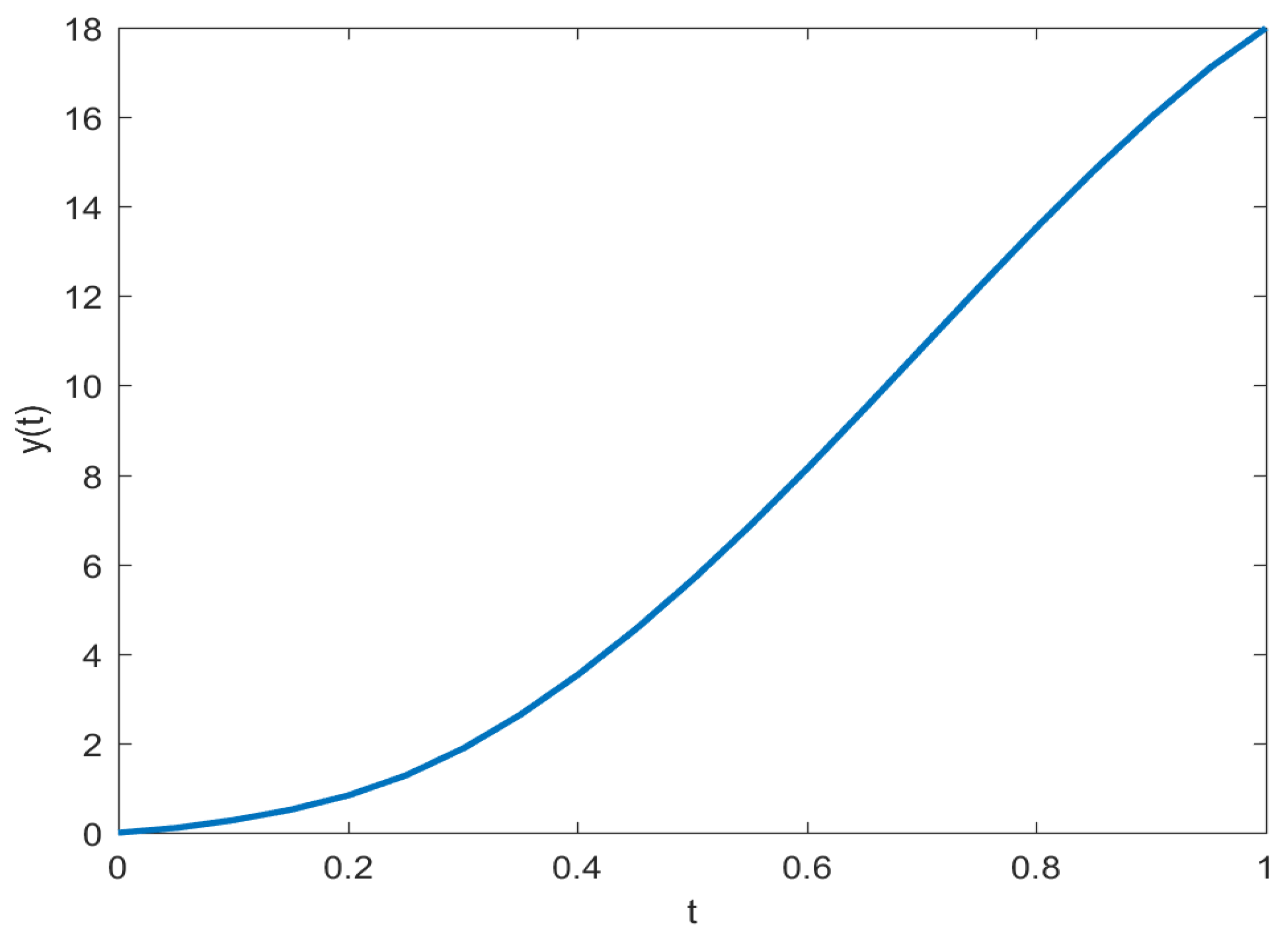
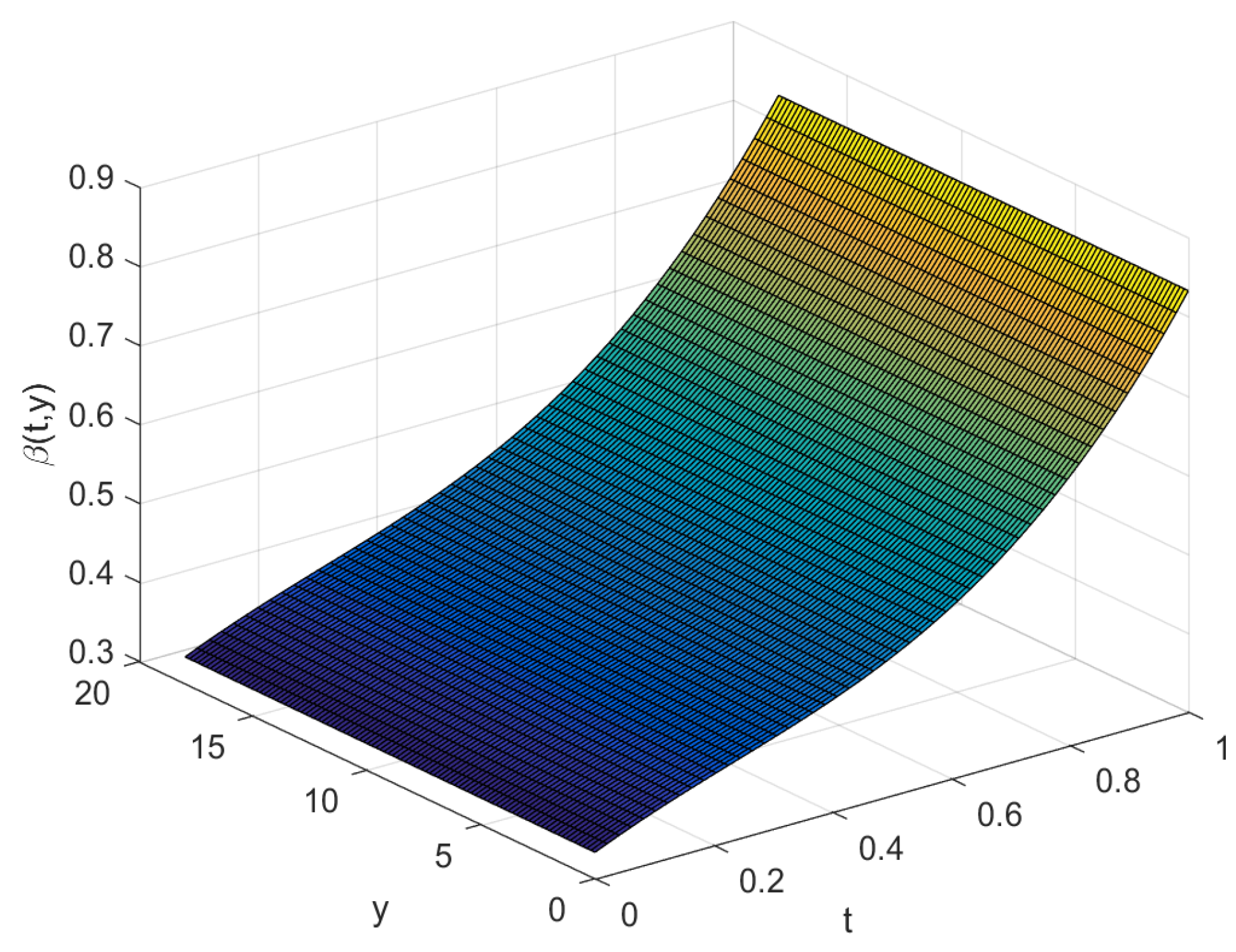
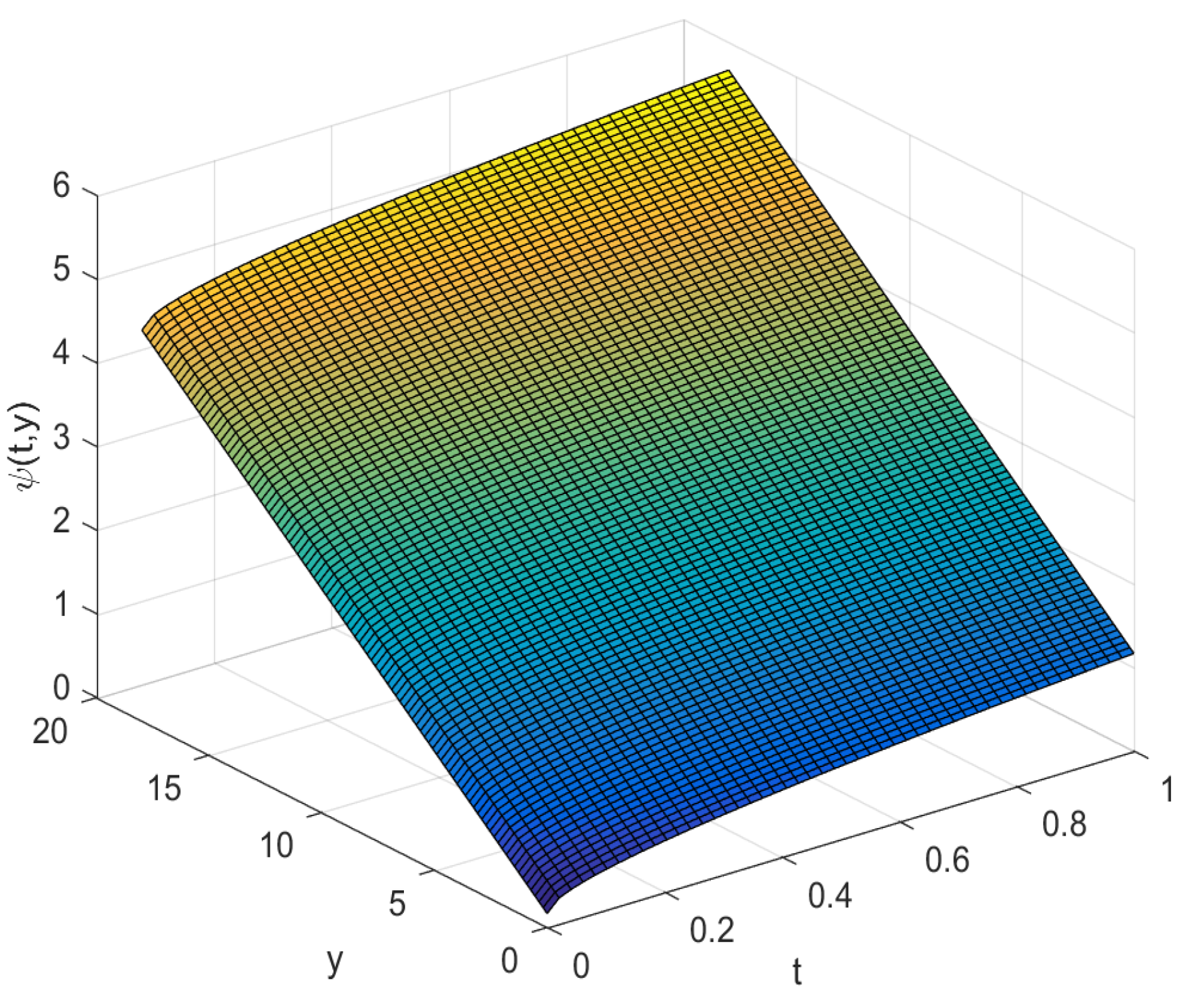
5. Approximate Numerical Applications

Example 1.

Let us consider the following fractional initial value problem

$$\left\{\begin{array}{ccc}{D}_{0^{+}}^{\beta (t,y(t\left)\right)}y\left(t\right)=\psi (t,y\left(t\right)),t\in \mathsf{\Delta }:=[0,1],\hfill & \left(A\right)\hfill & \\ & & \left(\mathrm{IVPNFDEVO}\right)\\ y\left(0\right)=0,\hfill & \left(B\right)\hfill & \end{array}\right.$$

with

$$\beta (t,y)=\frac{1}{4}\sqrt{t}+{\displaystyle \frac{1}{4(1+2y^3)}}$$

and

$$\psi (t,y\left(t\right))=\frac{e^{-t}\mid y\left(t\right)\mid }{(4+e^{2t})(1+\mid y\left(t\right)\mid )}.$$

We have that β is a continuous function on $\mathsf{\Delta }\times \mathbb{R}$ and $0<\beta (t,s)<1$.

Also,

$$\begin{array}{cc}\left|\psi \right(t,x)-\psi (t,y\left)\right|\hfill & {\displaystyle \le {\displaystyle \frac{e^{-t}}{(4+e^{2t})}}\left|\frac{x}{1+x}-\frac{y}{1+y}\right|}\hfill \\ \\ & {\displaystyle \le {\displaystyle \frac{e^{-t}|x-y|}{(4+e^{2t})(1+x)(1+y)}}}\hfill \\ \\ & {\displaystyle \le {\displaystyle \frac{e^{-t}}{(4+e^{2t})}}|x-y|}\hfill \\ \\ & {\displaystyle \le \frac{1}{5}|x-y|,}\hfill \end{array}$$

It is easy to check that for the given choice of nonlinear functions β and ψ Assumptions (A1) and (A2) are satisfied. Therefore, by Theorems 1 and 2, the problem (IVPNFDEVO) has a unique solution.

Example 2.

Let us consider the following fractional initial value problem

$$\left\{\begin{array}{ccc}{D}_{0^{+}}^{\beta (t,y(t\left)\right)}y\left(t\right)=\psi (t,y\left(t\right)),t\in \mathsf{\Delta }:=[0,1],\hfill & \left(A\right)\hfill & \\ & & \left(\mathrm{IVPNFDEVO}\right)\\ y\left(0\right)=0,\hfill & \left(B\right)\hfill & \end{array}\right.$$

with

$$\beta (t,y)=\frac{t^3}{3}+\frac{t}{3}+\frac{1}{3(y^2+1)}$$

and

$$\psi (t,y\left(t\right))=\frac{\mid y\left(t\right)\mid }{4}+\frac{1}{6}+\sqrt{t},t\in \mathsf{\Delta }.$$

We have that β is a continuous function on $\mathsf{\Delta }\times \mathbb{R}$ and $0<\beta (t,y)<1$.

Also,

$$\begin{array}{cc}\left|\psi \right(t,x)-\psi (t,y\left)\right|\hfill & {\displaystyle \le \left|\frac{\mid x\mid }{4}+\frac{1}{6}+\sqrt{t}-\left(\frac{\mid y\mid }{4}+\frac{1}{6}+\sqrt{t}\right)\right|}\hfill \\ \\ & {\displaystyle \le \left|\frac{\mid x\mid }{4}-\frac{\mid y\mid }{4}\right|}\hfill \\ \\ & {\displaystyle \le \frac{1}{4}|x-y|,x,y\in \mathbb{R}.}\hfill \end{array}$$

Hence, for the given choice of nonlinear functions β and ψ Assumptions (A1) and (A2) are satisfied. Therefore, by Theorems 1 and 2, the problem (IVPNFDEVO)) has a unique solution.

In the remaining part, some numerical applications are demonstrated.

The approximate solution $y\left(t\right)$ for ${\displaystyle \beta (t,y)=\frac{t^3}{3}+\frac{t}{3}+\frac{1}{3(y^2+1)}}$ with $t\in [0,1]$ is represented in Figure 1.

On the other hand, Figure 2 and Figure 3 present the graphs of the functions $\beta (t,y)$ and $\psi (t,y)$.

In

Table 1. Some values of $y\left(t\right)$ and $\beta (t,y)$ for $t\in [0,1]$.

t	0.1	0.2	0.3	0.4	0.5	0.6	0.7	0.8	0.9	1.0
$y\left(t\right)$	0.23	0.72	1.6	3.1	5.15	7.7	10.5	13.32	15.9	18
$\beta (t,y(t\left)\right)$	0.35	0.3	0.20	0.2	0.22	0.3	0.35	0.44	0.54	0.7

, we present our $\beta (t,y)$ and $y\left(t\right)$ with different value of $t\in [0,1]$.

6. Conclusions

In this study, we introduce an initial value problem for a class of nonlinear differential equations with fractional Riemann–Liouville-type derivative of variable nonlinear order. The existence and uniqueness of the solution are investigated in two different Banach spaces and new criteria are achieved. A Banach-type fixed point theorem is applied as a proof technique. In addition, a uniform stability result is established for the solution of the investigated problem which shows the efficiency of the existence criteria. The newly achieved outcomes complement results for different classes of variable-order fractional differential equations and provide an extension of the theory of such problems. Numerical applications are also elaborated. The introduced problem and the achieved results can be developed. Some directions of the future expansion of the topic include considering delay terms, reaction-diffusion terms and impulsive effects.

References

1. Baleanu, D.; Diethelm, K.; Scalas, E.; Trujillo, J.J. Fractional Calculus: Models and Numerical Methods, 1st ed.; World Scientific: Singapore, 2012; ISBN 978-981-4355-20-9. [Google Scholar]
2. Magin, R. Fractional Calculus in Bioengineering, 1st ed.; Begell House: Redding, CA, USA, 2006; ISBN 978-1567002157. [Google Scholar]
3. Kilbas, A.; Srivastava, H.M.; Trujillo, J.J. Theory and Applications of Fractional Differential Equations, 1st ed.; Elsevier: New York, NY, USA, 2006; ISBN 9780444518323. [Google Scholar]
4. Petráš, I. Fractional-Order Nonlinear Systems, 1st ed.; Springer: Heidelberg, Germany; Dordrecht, The Netherlands; London, UK; New York, NY, USA, 2011; ISBN 978-3-642-18101-6. [Google Scholar]
5. Samko, S.G.; Kilbas, A.A.; Marichev, O.I. Fractional Integrals and Derivatives: Theory and Applications, 1st ed.; Gordon and Breach: Yverdon, Switzerland, 1993; ISBN 9782881248641. [Google Scholar]
6. Stamova, I.M.; Stamov, G.T. Functional and Impulsive Differential Equations of Fractional Order: Qualitative Analysis and Applications, 1st ed.; Taylor & Francis Group: Boca Raton, FL, USA, 2017; ISBN 9781498764834. [Google Scholar]
7. Tarasov, V.E. Fractional Dynamics: Application of Fractional Calculus to Dynamics of Particles, Fields and Media, 1st ed.; Springer: Beijing, China, 2015; ISBN 978-3-642-14003-7. [Google Scholar]
8. Liouville, J. Mémoire sur quelques questions de géométrie et de mécanique, et sur un nouveau genre de calcul pour résoudre ces questions. J. Ec. Polytech. 1832, 13, 1–69. [Google Scholar]
9. Liouville, J. Mémoire sur le calcul des différentielles à indices quelconques. J. Ec. Polytech. 1832, 13, 71–162. [Google Scholar]
10. Heymans, N.; Podlubny, I. Physical interpretation of initial conditions for fractional differential equations with Riemann–Liouville fractional derivatives. Rheol. Acta 2006, 45, 765–771. [Google Scholar] [CrossRef]
11. Heymans, N.; Kitagawa, M. Modelling “unusual” behaviour after strain reversal with hierarchical fractional models. Rheol. Acta 2004, 43, 383–389. [Google Scholar] [CrossRef]
12. Koeller, R.C. Applications of fractional calculus to the theory of viscoelasticity. J. Appl. Mech. 1984, 51, 299–307. [Google Scholar] [CrossRef]
13. Schiessel, H.; Blumen, A. Hierarchical analogues to fractional relaxation equations. J. Phys. A 1993, 26, 5057–5069. [Google Scholar] [CrossRef]
14. Samko, S.; Ross, B. Integration and differentiation to a variable fractional order. Integral Transform. Spec. Funct. 1993, 1, 277–300. [Google Scholar] [CrossRef]
15. Lorenzo, C.F.; Hartley, T.T. Initialization, conceptualization, and application in the generalized fractional calculus. Crit. Rev. Biomed. Eng. 2007, 35, 477–553. [Google Scholar] [CrossRef]
16. Samko, S. Fractional integration and differentiation of variable order: An overview. Nonlinear Dyn. 2013, 71, 653–662. [Google Scholar] [CrossRef]
17. Sun, H.; Chang, A.; Zhang, Y.; Chen, W. A review on variable-order fractional differential equations: Mathematical foundations, physical models, numerical methods and applications. J. Fract. Calc. Appl. 2019, 22, 27–59. [Google Scholar] [CrossRef]
18. Valerio, D.; Costa, J.S. Variable-order fractional derivatives and their numerical approximations. Signal Process. 2011, 91, 470–483. [Google Scholar] [CrossRef]
19. Almeida, R.; Tavares, D.; Torres, D.F.M. The Variable-Order Fractional Calculus of Variations, 1st ed.; Springer: Cham, Switzerland, 2019; ISBN 978-3-319-94005-2. [Google Scholar]
20. Benkerrouche, A.; Souid, M.S.; Stamov, G.; Stamova, I. On the solutions of a quadratic integral equation of the Urysohn type of fractional variable order. Entropy 2022, 24, 886. [Google Scholar] [CrossRef]
21. Garrappa, R.; Giusti, A.; Mainardi, F. Variable-order fractional calculus: A change of perspective. Commun. Nonlinear Sci. Numer. Simul. 2021, 102, 105904. [Google Scholar] [CrossRef]
22. Odzijewicz, T.; Malinowska, A.B.; Torres, D.F.M. Fractional variational calculus of variable order. In Advances in Harmonic Analysis and Operator Theory, 1st ed.; Almeida, A., Castro, L., Speck, F.O., Eds.; Birkhäuser: Basel, Switzerland, 2013; Volume 229, pp. 291–301. [Google Scholar]
23. Zhang, S.; Hu, L. The existence of solutions and generalized Lyapunov-type inequalities to boundary value problems of differential equations of variable order. AIMS Math. 2020, 5, 2923–2943. [Google Scholar] [CrossRef]
24. Zhang, S.; Sun, S.; Hu, L. Approximate solutions to initial value problem for differential equation of variable order. J. Fract. Calc. Appl. 2018, 9, 93–112. [Google Scholar]
25. Ali, U.; Ahmad, H.; Abu-Zindah, H. Soliton solutions for nonlinear variable-order fractional Korteweg–de Vries (KdV) equation arising in shallow water waves. J. Ocean Eng. Sci. 2022. [Google Scholar] [CrossRef]
26. Patnaik, S.; Hollkamp, J.P.; Semperlotti, F. Applications of variable-order fractional operators: A review. Proc. R. Soc. A 2020, 476, 20190498. [Google Scholar] [CrossRef]
27. Lu, X.; Li, H.; Chen, N. An indicator for the electrode aging of lithium-ion batteries using a fractional variable order model. Electrochim. Acta 2019, 299, 378–387. [Google Scholar] [CrossRef]
28. Sun, H.G.; Chen, W.; Chen, Y.Q. Variable-order fractional differential operators in anomalous diffusion modeling. Physica A 2009, 388, 4586–4592. [Google Scholar] [CrossRef]
29. Sweilam, N.H.; AL-Mekhlafi, S.M.; Alshomrani, A.S.; Baleanu, D. Comparative study for optimal control nonlinear variable-order fractional tumor model. Chaos Solitons Fract. 2020, 136, 1–10. [Google Scholar] [CrossRef]
30. Zhuang, P.; Liu, F.; Anh, V.; Turner, I. Numerical methods for the variable-order fractional advection-diffusion equation with a nonlinear source term. SIAM J. Numer. Anal. 2009, 47, 1760–1781. [Google Scholar] [CrossRef]
31. Obembe, A.D.; Hossain, M.E.; Abu-Khamsin, S.A. Variable-order derivative time fractional diffusion model for heterogeneous porous media. J. Petrol. Sci. Eng. 2017, 152, 391–405. [Google Scholar] [CrossRef]
32. Diaz, G.; Coimbra, C.F.M. Nonlinear dynamics and control of a variable order oscillator with application to the van der Pol equation. Nonlinear Dynam. 2009, 56, 145–157. [Google Scholar] [CrossRef]
33. Zhang, H.; Liu, F.; Phanikumar, M.S.; Meerschaert, M.M. A novel numerical method for the time variable fractional order mobile-immobile advection-dispersion model. Comput. Math. Appl. 2013, 66, 693–701. [Google Scholar] [CrossRef]
34. Benkerrouche, A.; Baleanu, D.; Souid, M.S.; Hakem, A.; Inc, M. Boundary value problem for nonlinear fractional differential equations of variable order via Kuratowski MNC technique. Adv. Differ. Equ. 2021, 365, 1–19. [Google Scholar] [CrossRef]
35. Benkerrouche, A.; Souid, M.S.; Etemad, S.; Hakem, A.; Agarwal, P.; Rezapour, S.; Ntouyas, S.K.; Tariboon, J. Qualitative study on solutions of a Hadamard variable order boundary problem via the Ulam-Hyers-Rassias stability. Fractal Fract. 2021, 5, 108. [Google Scholar] [CrossRef]
36. Benkerrouche, A.; Souid, M.S.; Karapinar, E.; Hakem, A. On the boundary value problems of Hadamard fractional differential equations of variable order. Math. Meth. Appl. Sci. 2022, 46, 3187–3203. [Google Scholar] [CrossRef]
37. Benkerrouche, A.; Souid, M.S.; Sitthithakerngkiet, K.; Hakem, A. Implicit nonlinear fractional differential equations of variable order. Bound. Value Probl. 2021, 2021, 64. [Google Scholar] [CrossRef]
38. Benkerrouche, A.; Souid, M.S.; Stamov, G.; Stamova, I. Multiterm impulsive Caputo–Hadamard type differential equations of fractional variable order. Axioms 2022, 11, 634. [Google Scholar] [CrossRef]
39. Bouazza, Z.; Souid, M.S.; Hatira Günerhan, H. Multiterm boundary value problem of Caputo fractional differential equations of variable order. Adv. Differ. Equ. 2021, 2021, 1–17. [Google Scholar] [CrossRef]
40. Bouazza, Z.; Souid, M.S.; Etemad, S.; Kaabar, M.K.A. Darbo fixed point criterion on solutions of a Hadamard nonlinear variable order problem and Ulam-Hyers-Rassias stability. J. Funct. Spaces 2022, 2022, 1769359. [Google Scholar]
41. Refice, A.; Souid, M.S.; Stamova, I. On the boundary value problems of Hadamard fractional differential equations of variable order via Kuratowski MNC technique. Mathematics 2021, 9, 1134. [Google Scholar] [CrossRef]
42. Rezapour, S.; Souid, M.S.; Etemad, S.; Bouazza, Z.; Ntouyas, S.K.; Asawasamrit, S.; Tariboon, J. Mawhin continuation technique for a nonlinear BVP of variable order at resonance via piece-wise constant functions. Fractal Fract. 2021, 5, 216–230. [Google Scholar] [CrossRef]
43. Zhang, S. Existence of solutions for two-point boundary-value problems with singular differential equations of variable order. Electron. J. Differ. Equ. 2013, 2013, 1–16. [Google Scholar]
44. Kesavan, S. Functional Analysis, 1st ed.; Hindustan Book Agency: New Delhi, India, 2009; ISBN 978-93-86279-42-2. [Google Scholar]
45. Alsaedi, A.; Ahmad, B.; Alghamdi, B.; Ntouyas, S.K. On a nonlinear system of Riemann–Liouville fractional differential equations with semi-coupled integro-multipoint boundary conditions. Open Math. 2021, 19, 760–772. [Google Scholar] [CrossRef]
46. Abbas, S.; Benchohra, M.; Graef, J.R.; Henderson, J. Implicit Fractional Differential and Integral Equations: Existence and Stability, 1st ed.; Walter de Gruyter: Berlin, Germany, 2018; ISBN 9783110553130. [Google Scholar]
47. Benchohra, M.; Bouriah, S.; Nieto, J.J. Existence and Ulam stability for nonlinear implicit differential equations with Riemann–Liouville fractional derivative. Demonstr. Math. 2019, 52, 437–450. [Google Scholar] [CrossRef]
48. Luca, R. On a system of Riemann–Liouville fractional differential equations with coupled nonlocal boundary conditions. Adv. Differ. Equ. 2021, 2021, 134. [Google Scholar] [CrossRef]
49. Corduneanu, C. Principles of Differential and Integral Equations, 2nd ed.; AMS Chelsea Publishing: Providence, RI, USA, 2008; ISBN 978-0821846223. [Google Scholar]
Figure 1. The approximate solution y ( t ) in [ 0 , 1 ] with β ( t , y ) = t 3 3 + t 3 + 1 3 ( y 2 + 1 ) .
Axioms 12 00895 g001
Figure 2. The function β ( t , y ) for t [ 0 , 1 ] and y [ 0 , 20 ] .
Axioms 12 00895 g002
Figure 3. The function ψ ( t , y ) for t [ 0 , 1 ] and y [ 0 , 20 ] .
Axioms 12 00895 g003