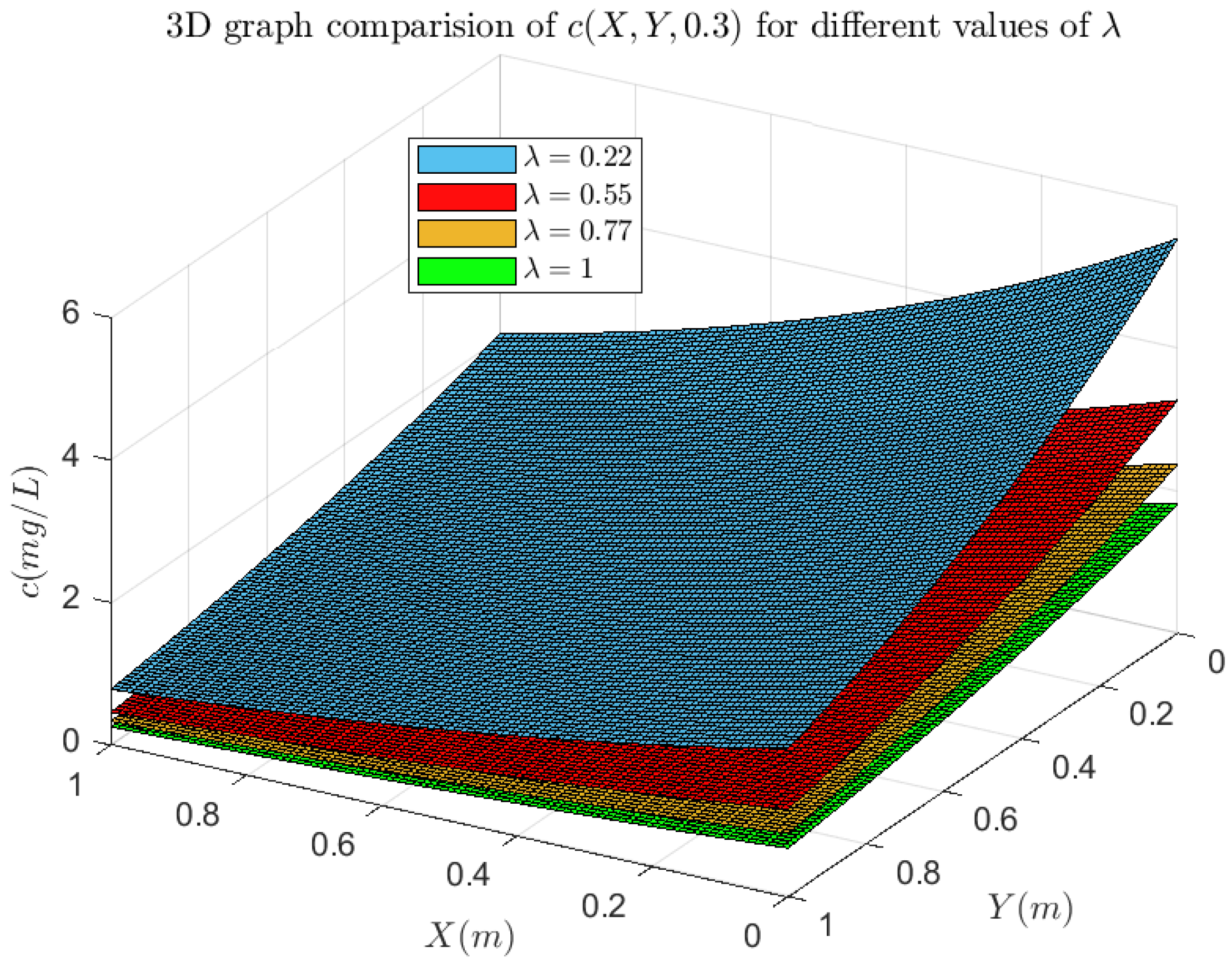
Article

Solution of Two-Dimensional Solute Transport Model for Heterogeneous Porous Medium Using Fractional Reduced Differential Transform Method

by
Manan A. Maisuria
1,
Priti V. Tandel
1,* and
Trushitkumar Patel
2
1
Department of Mathematics, Veer Narmad South Gujarat University, Surat 395007, India
2
Department of General Studies, University of the People, Pasadena, CA 91101, USA
*
Author to whom correspondence should be addressed.
Axioms 2023, 12(11), 1039; https://doi.org/10.3390/axioms12111039
Submission received: 10 October 2023 / Revised: 30 October 2023 / Accepted: 5 November 2023 / Published: 8 November 2023
(This article belongs to the Special Issue Fractional Calculus and the Applied Analysis)

Abstract

:
This study contains a two-dimensional mathematical model of solute transport in a river with temporally and spatially dependent flow, explicitly focusing on pulse-type input point sources with a fractional approach. This model is analyzed by assuming an initial concentration function as a declining exponential function in both the longitudinal and transverse directions. The governing equation is a time-fractional two-dimensional advection–dispersion equation with a variable form of dispersion coefficients, velocities, decay constant of the first order, production rate coefficient for the solute at the zero-order level, and retardation factor. The solution of the present problem is obtained by the fractional reduced differential transform method (FRDTM). The analysis of the initial retardation factor has been carried out via plots. Also, the influence of initial longitudinal and transverse dispersion coefficients and velocities has been examined by graphical analysis. The impact of fractional parameters on pollution levels is also analyzed numerically and graphically. The study of convergence for the FRDTM technique has been conducted to assess its efficacy and accuracy.

1. Introduction

Several authors have examined a space–time fractional partial differential equation. The fundamental partial differential equation may be changed by replacing the second-order space-derivative and first-order time-derivative with fractional derivatives of order β > 0 and α > 0 , respectively [1]. Authors have obtained a numerical solution of the one-dimensional fractional advection–dispersion equations with variable coefficients on a finite domain [2]. Fractional space derivatives represent anomalous diffusion or dispersion models, in which a particle plume spreads at a rate inconsistent with the classical Brownian motion model. In groundwater hydrology, fractional advection–dispersion equations represent passive tracer transfer in porous fluid flow. For a one-dimensional advection–dispersion model with constant coefficients, Fourier transform techniques provide analytical solutions [3,4].
Research on the transport of contaminants through porous media using hydraulic permeability is very significant for many technical, biophysical, and biological purposes. These include the treatment of contaminants, extraction of oil, and the management of high-level nuclear waste disposal [5]. Solute transport in disordered porous media is crucial in many scientific and engineering fields. Some of its examples are Tracer investigations in oil recovery, subsurface pollutant transfer, chemical transport in packed bed reactors, water filtering, fuel cells, and current catalyst development [6].
Several mathematical models have been created to study contaminant transport in porous media during groundwater flow, focusing on pollutant migration mechanisms. Djordjevich and Savovic have derived numerical solutions for the one-dimensional advection–diffusion equation with variable coefficients in semi-infinite media. The equation includes the dependence of flow on both time and space. The authors have used the explicit finite difference method to obtain the solution [7]. A numerical solution for two-dimensional solute transport was developed using finite difference techniques with periodic velocity in homogeneous porous media [8]. Two-dimensional solute transport was modeled mathematically in semi-infinite heterogeneous porous media. It has geographically and time-dependent coefficients for various input concentration pulses [9]. The Galerkin spectral element approach is used to provide an approximation of the Riesz space fractional in spatial directions, primarily to calculate the fractional advection–dispersion equation that applies in one and two dimensions of Riesz space [10]. For the alternative way to analyze the two-dimensional time distributed-order diffusion-wave equation, authors have also applied the Legendre–Laguerre spectral method over a semi-infinite domain [11]. The analysis of memory-based two-dimensional advection–diffusion equations inside a domain with a source located at the symmetry center of the domain is carried out by using Laplace and double sine-Fourier transformations [12].
There are multiple advantages to studying two-dimensional contaminant transport models over one-dimensional models. Two-dimensional models involve concentration gradients and contaminant transport in the orthogonal direction of the groundwater flow. Many researchers have analyzed two-dimensional models with longitudinal velocity components, neglecting the transverse velocity components. In the present problem, we have considered the dispersion coefficients as a linear multiple of spatially dependent function and seepage velocity and velocity components as the nth power of spatially dependent function. This is analyzed using the FRDTM, an advanced and effective method to identify solutions for the time-fractional two-dimensional advection–diffusion equation. Our research’s primary contribution is forecasting water behavior, which has significant implications for preserving water quality in environmental systems. We have also analyzed the effect of various factors on river pollution reduction.
In the context of modeling, fluid flow, and solute transport in porous media, the time-fractional part allows for the inclusion of subdiffusion phenomena. Subdiffusion refers to the phenomenon where the movement of fluid and solute particles is hindered, resulting in slower rates of advection and diffusion compared to classical scenarios. This hindrance may be attributed to many factors, such as obstacles or heterogeneities within the medium.
Fractional-order models provide greater flexibility in capturing complex dynamic behaviors due to their continuous nature, which can be more representative of real-world dynamics. Nonlinear fractional partial differential equations are often more challenging than linear ones. Moreover, no method gives an exact solution for the fractional-order differential equation. Hence, nonlinear PDEs of fractional order make the research more significant. They can describe systems with memory and hereditary properties more accurately. Fractional-order models explicitly capture non-local memory effects, while integer-order models assume local memory. However, there are some drawbacks to fractional-order models. They can be more mathematically complex and challenging to analyze compared to integer-order models. It requires specialized techniques to solve fractional-order differential equations.
In this paper, we have applied the latest technique, namely the FRDTM—an efficient and robust method to find the solutions of the time-fractional two-dimensional advection–dispersion equation. The FRDTM provides highly accurate numerical results for nonlinear time-fractional differential equations without spatial discretization, linearization, transformation, or perturbation. The FRDTM can be applied to derive a variety of fractional-order nonlinear problems with distinct physical structures arising in science, which is the novelty of our work.
The remainder of this paper is structured as follows: Section 2 discusses the mathematical construction of the model. Section 3 revisits several fundamental concepts and features of the FRDTM. Section 4 discusses the numerical results and their consequences. Section 5 closes with concluding comments.

2. Mathematical Construction of the Problem

The two primary mechanisms by which contaminants penetrate the subsurface are advection, which is brought on by groundwater movement, and dispersion, which results from mechanical mixing and molecular diffusion, both occurring simultaneously. The small seepage velocity precludes the investigation of molecular diffusions. The two-dimensional advection–diffusion equation can have its mathematical form provided by a parabolic partial differential equation of the second order. It is expressed as [13]
R c τ = x D x c x u c + y D y c y v c α c + β
The variable c (mg L 1 ) represents the solute concentration of the pollutant as it is transported through the medium along the flow field at any given place ( x , y ) and time τ . D x (m 2 day 1 ) and D y (m 2 day 1 ) represent the longitudinal and transverse dispersion coefficients, respectively. Additionally, the parameters u (m day 1 ) and v (m day 1 ) values represent the unstable uniform seepage velocity in the longitudinal and transverse directions, respectively. The value α (day 1 ) represents the decay constant of the first order, while the parameter β (kg m 3 day 1 ) identifies the production rate coefficient for the solute at the zero-order level which represents the production of the solute internally or externally in the medium. The dimensionless quantity known as the retardation factor is symbolized by R .
Consider the spatial and temporal dependencies of the flow domain parameters as under [13]
D x = D x 0 ( 1 + a x ) 3 ( 1 + b y ) g ( m τ ) , D y = D y 0 ( 1 + b y ) 3 ( 1 + a x ) g ( m τ ) , u = u 0 ( 1 + a x ) 2 ( 1 + b y ) g ( m τ ) , v = v 0 ( 1 + b y ) 2 ( 1 + a x ) g ( m τ ) , R = R 0 ( 1 + a x ) ( 1 + b y ) , α = α 0 ( 1 + a x ) ( 1 + b y ) g ( m τ ) , β = β 0 ( 1 + a x ) ( 1 + b y ) g ( m τ )
The parameters a and b represent heterogeneity in the longitudinal and transverse directions. The varied values of a and b reflect various levels of heterogeneity. The heterogeneity of the porous media refers to the condition where the porosity or hydraulic conductivity varies based on the specific location within the medium. Initial dispersion coefficients in the longitudinal and transverse directions are denoted by the symbols D x 0 and D y 0 , respectively. Initial unstable uniform seepage velocities in the longitudinal and lateral directions are denoted by the notation u 0 and v 0 , respectively. The parameter for unsteadiness is denoted by m. The initial decay constant of the first order and the zero-order production rate coefficient for the solute are denoted by the notations α 0 and β 0 , respectively. R 0 is the initial retardation factor. We assumed g ( m τ ) , where g ( m τ ) = 1 when τ = 0 or m = 0 . The first situation depicts a steady flow, while the second represents the initial state. g ( m τ ) is an expression without dimensions. Therefore, Equation (1) is converted into the given form.
R 0 g ( m τ ) c τ = D x 0 ( 1 + a x ) 2 2 c x 2 + D y 0 ( 1 + b y ) 2 2 c y 2 + 3 D x 0 a u 0 ( 1 + a x ) c x + 3 D y 0 b v 0 ( 1 + b y ) c y 2 ( a u 0 + b v 0 ) c α 0 c + β 0
Let us introduce new variables defined as under [13].
X = l o g ( 1 + a x ) a ,   Y = l o g ( 1 + b y ) b   and   T = 0 τ g ( m τ ) d τ .
Hence, Equation (3) transforms into the given form using the provided transformations.
R 0 c T = D x 0 2 c X 2 + D y 0 2 c Y 2 ( u 0 2 a D x 0 ) c X ( v 0 2 b D y 0 ) c Y 2 ( a u 0 + b v 0 ) c α 0 c + β 0
The initial values of the function c ( X , Y , T ) are supposed to follow a declining exponential pattern with respect to both X and Y [14].
c ( X , Y , 0 ) = e ( X + Y ) γ 0

3. Fractional Reduced Differential Transform Method (FRDTM)

Some of the basic ideas and characteristics of the theory of fractional calculus are explained in this section [15,16].
Definition 1.
The fractional derivative of the function w of order λ, in the sense of Caputo, is denoted by D λ w ( τ ) and is defined as
D λ w ( τ ) = 1 Γ ( n λ ) 0 1 ( τ t ) w n ( t ) d t , f o r n 1 < λ n , n N
Let us consider a function of three variables, denoted as ω ( ϑ , ϖ , τ ) , which can be expressed as the product of three single-variable functions, i.e., ω ( ϑ , ϖ , τ ) = s ( ϑ ) k ( ϖ ) u ( τ ) . The representation of function ω ( ϑ , ϖ , τ ) may be determined based on the characteristics of differential transform.
ω ( ϑ , ϖ , τ ) = n = 0 Ω n ( ϑ , ϖ ) τ λ n
where Ω n ( ϑ , ϖ ) is a t-dimensional spectrum function. Ω n ( ϑ , ϖ ) is the transformed function of ω ( ϑ , ϖ , τ ) . The basic definitions and operations of the FRDTM are as follows:
The R D operator signifies the reduced differential transform, whereas the R D 1 denotes the inverse reduced differential transform.
Definition 2.
Let us examine the function ω ( ϑ , ϖ , τ ) , which is assumed to possess analyticity and continuous differentiability with respect to ϑ, ϖ, and τ inside the selected domain. The definition of the reduced differential transformations for the function ω ( ϑ , ϖ , τ ) is as follows [17,18]:
R D ω ( ϑ , ϖ , τ ) Ω n ( ϑ , ϖ ) = 1 Γ ( λ n + 1 ) λ n τ λ n ω ( ϑ , ϖ , τ ) τ = 0
The symbol λ is used to denote the time-fractional-order derivative.
Definition 3.
The following is a presentation of the inverse differential transformations of the function Ω n ( ϑ , ϖ ) :
R D 1 Ω n ( ϑ , ϖ ) ω ( ϑ , ϖ , τ ) = n = 0 Ω n ( ϑ , ϖ ) τ λ n
From Equations (8) and (9), we obtain
ω ( ϑ , ϖ , τ ) = n = 0 1 Γ ( λ n + 1 ) λ n τ λ n ω ( ϑ , ϖ , τ ) τ = 0 τ λ n
In order to elucidate the fundamental principles of the FRDTM, let us examine the following nonlinear partial differential equation expressed in an operator format [19]:
L ω ( ϑ , ϖ , τ ) + H ω ( ϑ , ϖ , τ ) + W ω ( ϑ , ϖ , τ ) = f ( ϑ , ϖ , τ )
with initial condition
ω ( ϑ , ϖ , 0 ) = h ( ϑ , ϖ )
where L = λ τ λ , the linear operator H has partial derivatives, whereas the operator W ω ( ϑ , ϖ , τ ) is nonlinear, and f ( ϑ , ϖ , τ ) represents an inhomogeneous term.
Based on the principles of the FRDTM, it is possible to derive the following iteration formula:
Γ ( λ ( n + 1 ) + 1 ) Γ ( λ n + 1 ) Ω n + 1 ( ϑ , ϖ ) = F n ( ϑ , ϖ ) H Ω n ( ϑ , ϖ ) W Ω n ( ϑ , ϖ )
The functions Ω n ( ϑ , ϖ ) , H Ω n ( ϑ , ϖ ) , W Ω n ( ϑ , ϖ ) , and F n ( ϑ , ϖ ) represent the transformations of the functions ω ( ϑ , ϖ , τ ) , H ω ( ϑ , ϖ , τ ) , W ω ( ϑ , ϖ , τ ) , and f ( ϑ , ϖ , τ ) , respectively.
Based on the initial condition (12), we formulate
Ω 0 ( ϑ , ϖ ) = h ( ϑ , ϖ )
By substituting Equation (14) into Equation (13) and conducting a basic iterative computation, we get the values of Ω n ( ϑ , ϖ ) as follows. Subsequently, the inverse translation of the set of values Ω n ( ϑ , ϖ ) n = 0 k yields the k-terms approximation solution in the following manner:
ω k ( ϑ , ϖ , τ ) = n = 0 k Ω n ( ϑ , ϖ ) τ λ n
Hence, the exact answer is given by
ω ( ϑ , ϖ , τ ) = lim k ω k ( ϑ , ϖ , τ )
Theorem 1.
If ω ( ϑ , ϖ , τ ) = n = 0 Ω n ( ϑ , ϖ ) τ λ n is given series [20,21,22]:
1. 
Given series solution is convergent if 0 < α < 1 such that Ω n + 1 Ω n α .
2. 
Given series solution is divergent if α > 1 such that Ω n + 1 Ω n α .
The proof of Theorem 1, which is a particular case of Banach’s fixed point theorem, can be found in the reference.
Corollary 1.
The series solution n = 0 Ω n ( ϑ , ϖ , τ ) exhibits convergence toward the exact solution ω ( ϑ , ϖ , τ ) with the condition that 0 ξ k < 1 , where every k belongs to the whole number [20,21,22].
ξ k = Ω k + 1 Ω k , Ω k 0 0 , Ω k = 0
Table 1 presents the essential mathematical operations of the FRDTM, providing simple accessibility.

4. Results and Discussion

This part illustrates the numerical and graphical outcomes of the derived general solution, which includes several parameters. The impact of various parameters on the concentration profile has also been observed. In order to analyze this, Equation (4) was transformed into time-fractional partial differential equations, which are presented as follows:
R 0 λ c T λ = D x 0 2 c X 2 + D y 0 2 c Y 2 ( u 0 2 a D x 0 ) c X ( v 0 2 b D y 0 ) c Y 2 ( a u 0 + b v 0 ) c α 0 c + β 0
Applying the FRDTM on both sides of Equation (17), we obtain
R 0 Γ ( λ ( n + 1 ) + 1 ) Γ ( λ n + 1 ) C n + 1 = D x 0 2 C n X 2 + D y 0 2 C n Y 2 ( u 0 2 a D x 0 ) C n X ( v 0 2 b D y 0 ) C n Y 2 ( a u 0 + b v 0 ) C n α 0 C n + β 0 δ ( n λ )
C n + 1 = Γ ( λ n + 1 ) R 0 Γ ( λ ( n + 1 ) + 1 ) [ D x 0 2 C n X 2 + D y 0 2 C n Y 2 ( u 0 2 a D x 0 ) C n X ( v 0 2 b D y 0 ) C n Y 2 ( a u 0 + b v 0 ) C n α 0 C n + β 0 δ ( n λ ) ]
From the initial condition (5), we obtain
C 0 = e ( X + Y ) γ 0
From Equation (19) and (20), we obtain the general solution
c ( X , Y , T ) = C 0 ( X , Y ) + C 1 ( X , Y ) T λ + C 2 ( X , Y ) T λ 2 + = Φ 0 + Φ 1 + Φ 2 +
where
C 0 = e ( X + Y ) γ 0 C 1 = e X + Y γ 0 D x 0 + D y 0 + γ 0 u 0 + γ 0 v 0 α 0 γ 0 2 + γ 0 2 β 0 e X + Y γ 0 2 a D x 0 γ 0 2 b D y 0 γ 0 2 a γ 0 2 u 0 2 b γ 0 2 v 0 γ 0 2 R 0 Γ λ + 1 C 2 = e X + Y γ 0 α 0 + 2 a u 0 + 2 b v 0 α 0 + 2 a u 0 + 2 b v 0 β 0 e X + Y γ 0 R 0 2 Γ 2 λ + 1 + e X + Y γ 0 D x 0 + D y 0 2 γ 0 4 R 0 2 Γ 2 λ + 1 e X + Y γ 0 4 a 2 D x 0 2 8 a b D x 0 D y 0 + 8 a D x 0 u 0 + 4 a D x 0 v 0 + 4 a D y 0 u 0 4 b 2 D y 0 2 + 4 b D x 0 v 0 + 4 b D y 0 u 0 + 8 b D y 0 v 0 + 2 α 0 D x 0 + 2 α 0 D y 0 u 0 2 2 u 0 v 0 v 0 2 γ 0 2 R 0 2 Γ 2 λ + 1 + 2 e X + Y γ 0 D x 0 + D y 0 u 0 + v 0 2 a D x 0 2 b D y 0 γ 0 3 R 0 2 Γ 2 λ + 1 2 e X + Y γ 0 α 0 + 2 a u 0 + 2 b v 0 u 0 + v 0 2 a D x 0 2 b D y 0 γ 0 R 0 2 Γ 2 λ + 1
Furthermore, in order to perform a convergence analysis of a given series solution, we calculate the terms ξ k using corollary 1. ξ 0 = Φ 1 Φ 0 = 0.2057 < 1 , ξ 1 = Φ 2 Φ 1 = 0.2054 < 1 . This observation confirms that the FRDTM yields a series solution that exhibits convergence toward the exact solution. Now, we have obtained the numerical values of the concentration for fixed R 0 = 1.15 , u 0 = 1.05 , v 0 = 0.105 , α 0 = 0.01 , D x 0 = 1.25 , D y 0 = 0.125 , γ 0 = 1.02 , a = b = 0.01 and β 0 = 0.0021 [13].
Table 2, Table 3 and Table 4 give the numerical values of concentration at fixed ( Y = 0.33 , T = 0.2 ) , ( Y = 0.55 , T = 0.4 ) , and ( Y = 0.77 , T = 0.3 ) for different values of λ , respectively. We have shown a negative correlation between the change in X and the change in concentration. As Y continues to rise, the concentration will continue to fall. If there is an increase in T, there is also an increase in concentration. Additionally, we saw that the concentration was becoming lower as the λ value increased.
Figure 1 presents a three-dimensional depiction of the concentration profile at various time points ( T ) . Figure 2 and Figure 3 provide visual depictions of concentration variations for distinct values of X and Y, respectively. The value of variable c exhibits a positive correlation with the value of variable T, wherein a rise in T results in a corresponding increase in the value of c. The value of variable c exhibits a negative correlation with the values of variables X and Y as the latter two variables grow.
The graphical depiction of concentration for various fractional order values ( λ = 0.22 ,   0.55 ,   0.77 ,   1 ) at a constant period ( T = 0.3 ) is shown in Figure 4. As the value of λ increases from 0 to 1, the value of c decreases.
Figure 5 presents a visual depiction of the impact of the retardation factor on the concentration of pollutants. Table 5 and Table 6 give the numerical values of pollutant concentration for different initial retardation factor R 0 = 1.15 and R 0 = 2.25 , respectively, for fixed parameters u 0 = 1.05 ,   v 0 = 0.105 ,   α 0 = 0.04 ,   D x 0 = 1.25 ,   D y 0 = 0.125 ,   a = b = 0.01 ,   T = 0.5 ,   γ 0 = 1.02 and β 0 = 0.0021 .
Figure 6 presents a three-dimensional graphical depiction illustrating the impact of initial velocity on the concentration of pollutants. Table 7 and Table 8 present numerical values of the concentration function for various initial velocities. The values of ( u 0 ,   v 0 ) are ( 1.05 ,   0.105 ) and ( 2.5 ,   0.25 ) , respectively, for the specified parameters. The values of the parameters are as follows: R 0 = 1.15 ,   α 0 = 0.04 ,   D x 0 = 1.25 ,   D y 0 = 0.125 ,   a = b = 0.01 ,   T = 0.4 ,   γ 0 = 1.02 , and β 0 = 0.0021 .
Figure 7 provides a visual depiction of the impact of the dispersion coefficient on the concentration of pollutants. The numerical values of the concentration profile for different initial dispersion coefficients at various space and time intervals are shown in Table 9 and Table 10. The value of initial dispersion coefficients ( D x 0 , D y 0 ) are ( 1.25 , 0.125 ) and ( 2.5 , 0.25 ) , respectively, for the fixed parameters R 0 = 1.15 ,   u 0 = 1.05 ,   v 0 = 0.105 ,   α 0 = 0.04 ,   a = b = 0.01 ,   T = 0.8 ,   γ 0 = 1.02 , and β 0 = 0.0021 . The concentration function’s value ( c ) drops as R 0 rises. The value of the concentration function ( c ) rises when ( D x 0 , D y 0 ) and ( u 0 , v 0 ) in the longitudinal and transverse directions are increased.

5. Conclusions

The efficacy of using the fractional reduced differential transform method (FRDTM) has been shown in acquiring a two-dimensional analytical solution for the advection–dispersion problem. This approach can handle variable parameters and is used explicitly for nonreactive pollutant transport. Additionally, the FRDTM approach demonstrates a more rapid convergence of the solutions. The level of concentration has a positive correlation with the increase in time. The concentration negatively correlates with the rise in variables X and Y. When the initial retardation factor rises, there is a corresponding fall in pollutant levels. When the starting velocity and dispersion coefficient rise, there is a corresponding increase in the pollutant level. The impact of the fractional order of the Caputo derivative on the concentration of pollutants is significant. In the context of the present study, it is observed that, when the fractional order is smaller, there is an increase in the concentration of pollutants within the specified research area. The discovered solution demonstrates excellent applicability to actual instances of solute transport phenomena. An analytic solution is essential and cost-effective because it offers a more accurate physical understanding of water transport and solutes. This study will demonstrate that several methods have been provided to address this specific real-life problem to demonstrate the efficacy and efficiency of the procedure under consideration.

Author Contributions

All authors have contributed equally to the manuscript. All authors have read and agreed to the published version of the manuscript.

Funding

This research received no external funding.

Institutional Review Board Statement

Not applicable.

Informed Consent Statement

Not applicable.

Data Availability Statement

Data are contained within the article.

Conflicts of Interest

The authors declare no conflict of interest.

References

  1. Liu, F.; Anh, V.V.; Turner, I.; Zhuang, P. Time fractional advection-dispersion equation. J. Appl. Math. Comput. 2003, 13, 233–245. [Google Scholar] [CrossRef]
  2. Mark, M.M.; Charles, T. Finite difference approximations for fractional advection-dispersion flow equations. J. Comput. Appl. Math. 2004, 172, 65–77. [Google Scholar]
  3. Chaves, A.S. A fractional diffusion equation to describe Lévy flights. Phys. Lett. A 1998, 239, 13–16. [Google Scholar] [CrossRef]
  4. Benson, D.A.; Wheatcraft, S.W.; Meerschaert, M.M. Application of a fractional advection-dispersion equation. Water Resour. Res. 2000, 36, 1403–1412. [Google Scholar] [CrossRef]
  5. Natarajan, N.; Kumar, G.S. Spatial moment analysis of colloid facilitated radionuclide transport in a coupled fracture-matrix system. Int. J. Energy Environ. 2011, 2, 491–504. [Google Scholar]
  6. Ovaysi, S.; Piri, M.C. Pore-scale modeling of dispersion in disordered porous media. J. Contam. Hydrol. 2011, 124, 68–81. [Google Scholar] [CrossRef]
  7. Savovic, S.; Djordjevich, A. Numerical solution for temporally and spatially dependent solute dispersion of pulse type input concentration in semi-infinite media. Int. J. Heat Mass Transf. 2013, 60, 291–295. [Google Scholar] [CrossRef]
  8. Djordjevich, A.; Savovic, S.; Janicijevic, A. Explicit finite-difference solution of two-dimensional solute transport with periodic flow in homogenous porous media. J. Hydrol. Hydromech. 2017, 65, 426–432. [Google Scholar] [CrossRef]
  9. Yadav, R.R.; Kumar, L.K. Two-dimensional conservative solute transport with temporal and scale-dependent dispersion: Analytical solution. Int. J. Adv. Math. 2018, 2, 90–111. [Google Scholar]
  10. Saffarian, M.; Mohebbi, A. Finite difference/spectral element method for one and two-dimensional Riesz space fractional advection–dispersion equations. Math. Comput. Simul. 2022, 193, 348–370. [Google Scholar] [CrossRef]
  11. Zhang, H.; Liu, F.; Jiang, X.; Turner, I. Spectral method for the two-dimensional time distributed-order diffusion-wave equation on a semi-infinite domain. J. Comput. Appl. Math. 2022, 399, 113712. [Google Scholar] [CrossRef]
  12. Ahmed, N.; Shah, N.A.; Vieru, D. Two-dimensional advection–diffusion process with memory and concentrated source. Symmetry 2019, 11, 879. [Google Scholar] [CrossRef]
  13. Yadav, R.R.; Kumar, L.K. Solute transport for pulse type input point source along temporally and spatially dependent flow. Pollution 2019, 5, 53–70. [Google Scholar]
  14. Hadhouda, M.K.; Hassan, Z.S. Mathematical model for unsteady remediation of river pollution by aeration. Inf. Sci. Lett. 2022, 11, 323–329. [Google Scholar]
  15. Patel, H.; Patel, T.; Pandit, D. An efficient technique for solving fractional-order diffusion equations arising in oil pollution. J. Ocean. Eng. Sci. 2023, 8, 217–225. [Google Scholar] [CrossRef]
  16. Alshammari, S.; Abuasad, S. Exact solutions of the 3D fractional helmholtz equation by fractional differential transform method. J. Funct. Spaces 2022, 2022, 7374751. [Google Scholar] [CrossRef]
  17. Patel, T.; Patel, H. An analytical approach to solve the fractional-order (2+1)-dimensional Wu–Zhang equation. Math. Methods Appl. Sci. 2023, 46, 479–489. [Google Scholar] [CrossRef]
  18. Osman, M.; Xia, Y.; Omer, O.A.; Hamoud, A. On the fuzzy solution of linear-nonlinear partial differential equations. Mathematics 2022, 10, 2295. [Google Scholar] [CrossRef]
  19. Al-Amr, M.O. New applications of reduced differential transform method. Alex. Eng. J. 2014, 53, 243–247. [Google Scholar] [CrossRef]
  20. Moosavi Noori, S.R.; Taghizadeh, N. Study of convergence of reduced differential transform method for different classes of differential equations. Int. J. Differ. Equations 2021, 2021, 6696414. [Google Scholar] [CrossRef]
  21. Noori, S.R.M.; Taghizadeh, N. Study of convergence of reduced differential transform method for different classes of nonlinear differential equations. Authorea Prepr. 2020. [Google Scholar] [CrossRef]
  22. Varsoliwala, A.C.; Singh, T.R. Mathematical modeling of atmospheric internal waves phenomenon and its solution by Elzaki Adomian decomposition method. J. Ocean. Eng. Sci. 2022, 7, 203–212. [Google Scholar] [CrossRef]
  23. Tandel, P.; Patel, H.; Patel, T. Tsunami wave propagation model: A fractional approach. J. Ocean. Eng. Sci. 2022, 7, 509–520. [Google Scholar] [CrossRef]
  24. Singh, B.K.; Kumar, P. FRDTM for numerical simulation of multi-dimensional, time-fractional model of Navier–Stokes equation. Ain Shams Eng. J. 2018, 9, 827–834. [Google Scholar] [CrossRef]
  25. Abuasad, S.; Moaddy, K.; Hashim, I. Analytical treatment of two-dimensional fractional Helmholtz equations. J. King Saud-Univ.-Sci. 2019, 31, 659–666. [Google Scholar] [CrossRef]
  26. Al-rabtah, A.; Abuasad, S. Effective Modified Fractional Reduced Differential Transform Method for Solving Multi-Term Time-Fractional Wave-Diffusion Equations. Symmetry 2023, 15, 1721. [Google Scholar] [CrossRef]
Figure 1. Three-dimensional comparison of approximate solution for different values of T = 0.2 ,   0.5 ,   0.7 , and 0.9 for R 0 = 1.15 ,   u 0 = 1.05 ,   v 0 = 0.105 ,   α 0 = 0.04 ,   D x 0 = 1.25 ,   D y 0 = 0.125 ,   a = b = 0.01 ,   λ = 1 ,   γ 0 = 1.02 , and β 0 = 0.0021 .
Axioms 12 01039 g001
Figure 2. Two-dimensional comparison of approximate solution for different values of X = 0.1 ,   0.4 ,   0.7 , and 1 for R 0 = 1.15 ,   u 0 = 1.05 ,   v 0 = 0.105 ,   α 0 = 0.04 ,   D x 0 = 1.25 ,   D y 0 = 0.125 ,   a = b = 0.01 ,   λ = 1 ,   γ 0 = 1.02 , and β 0 = 0.0021 .
Axioms 12 01039 g002
Figure 3. Two-dimensional comparison of approximate solution for different values of Y = 0.2 ,   0.5 ,   0.8 , and 1 for R 0 = 1.15 ,   u 0 = 1.05 ,   v 0 = 0.105 ,   α 0 = 0.04 ,   D x 0 = 1.25 ,   D y 0 = 0.125 ,   a = b = 0.01 ,   λ = 1 ,   γ 0 = 1.02 , and β 0 = 0.0021 .
Axioms 12 01039 g003
Figure 4. Behavior of approximate solution for different values of λ = 0.22 ,   0.55 ,   0.77 , and 1 for R 0 = 1.15 ,   u 0 = 1.05 ,   v 0 = 0.105 ,   α 0 = 0.04 ,   D x 0 = 1.25 ,   D y 0 = 0.125 ,   a = b = 0.01 ,   T = 0.3 ,   γ 0 = 1.02 , and β 0 = 0.0021 .
Axioms 12 01039 g004
Figure 5. Comparison of the concentration profile in three dimensions for various retardation coefficients R 0 = 1.15 ,   1.85 ,   2 , and 2.25 for u 0 = 1.05 ,   v 0 = 0.105 ,   α 0 = 0.04 ,   D x 0 = 1.25 ,   D y 0 = 0.125 ,   a = b = 0.01 ,   T = 0.5 ,   γ 0 = 1.02 , and β 0 = 0.0021 .
Axioms 12 01039 g005
Figure 6. Comparison of the concentration profile in three dimensions for various initial velocities ( u 0 = 1.05 ,   v 0 = 0.105 ) , ( u 0 = 1.85 ,   v 0 = 0.185 ) , and ( u 0 = 2.5 ,   v 0 = 0.25 ) for R 0 = 1.15 ,   α 0 = 0.04 ,   D x 0 = 1.25 ,   D y 0 = 0.125 ,   a = b = 0.01 ,   T = 0.4 ,   γ 0 = 1.02 , and β 0 = 0.0021 .
Axioms 12 01039 g006
Figure 7. Comparison of the concentration profile in three dimensions for various initial dispersion coefficients ( D x 0 = 1.25 ,   D y 0 = 0.125 ) , ( D x 0 = 1.85 ,   D y 0 = 0.185 ) , and ( D x 0 = 2.5 ,   D y 0 = 0.25 ) for R 0 = 1.15 ,   u 0 = 1.05 ,   v 0 = 0.105 ,   α 0 = 0.04 ,   a = b = 0.01 ,   T = 0.8 ,   γ 0 = 1.02 , and β 0 = 0.0021 .
Axioms 12 01039 g007
Table 1. Transform table [23,24,25,26].
FunctionTransformation
ω ( ϑ , ϖ , τ ) Ω j ( ϑ , ϖ ) = 1 Γ ( λ j + 1 ) λ j τ λ j ω ( ϑ , ϖ , τ ) τ = 0
α ϕ ± β ξ α Φ j ± β Ξ j , α and β are constant.
ϕ ( ϑ , ϖ , τ ) ξ ( ϑ , ϖ , τ ) n = 0 j Φ n ( ϑ , ϖ ) Ξ j n ( ϑ , ϖ )
λ n τ λ n ω ( ϑ , ϖ , τ ) Γ ( j λ + n λ + 1 ) Γ ( j λ + 1 ) Ω j + n ( ϑ , ϖ )
n ϑ n ω ( ϑ , ϖ , τ ) n ϑ n Ω j ( ϑ , ϖ ) .
n ϖ n ω ( ϑ , ϖ , τ ) n ϖ n Ω j ( ϑ , ϖ ) .
ϑ m ϖ p τ n ϑ m ϖ p δ ( j λ n ) where δ ( j λ n ) = 1 j λ = n 0 , j λ n .
Table 2. c ( X , 0.33 , 0.2 ) .
X λ = 0.11 λ = 0.33 λ = 0.66 λ = 0.88 λ = 1
0.13.9804776072.6073434651.4541814551.0996316730.98151519
0.23.608897742.3639610351.3184447520.9969837330.88988869
0.33.2720184722.1433072761.1953840450.9039217410.80681889
0.42.966599231.9432596321.0838155650.8195504970.7315067
0.52.6897020691.7618937670.9826660920.74305840.66322765
0.62.4386634061.5974650530.890962630.6737096440.60132496
0.72.2110684021.4483917860.8078230460.6108371370.54520316
0.82.0047277341.3132399710.732447590.5538360820.49432238
0.91.8176565291.1907095320.6641111960.5021581640.44819319
11.6480552781.0796218010.6021565080.4553062750.40637185
Table 3. c ( X , 0.55 , 0.4 ) .
X λ = 0.11 λ = 0.33 λ = 0.66 λ = 0.88 λ = 1
0.13.5676497742.7826920861.7526397461.3123384021.1429389
0.23.2346332782.52296121.5890675311.1898620871.03627113
0.32.9327160772.2874857121.4407707781.0788234250.93956471
0.42.6589939122.074000491.3063229610.9781542910.85188937
0.52.4108337431.8804519381.1844307760.8868863110.77240174
0.62.1858484211.7049782381.0739216940.8041415420.70033719
0.71.9818737251.5458914380.9737326850.7291240290.63500251
0.81.7969475421.4016612220.8828999910.6611121510.57576922
0.91.6292909961.2709001820.8005498590.5994516750.52206752
11.4772913341.1523504780.725890130.5435494630.47338085
Table 4. c ( X , 0.77 , 0.3 ) .
X λ = 0.11 λ = 0.33 λ = 0.66 λ = 0.88 λ = 1
0.12.7508522311.9887018371.1771286140.8781666510.77053285
0.22.4941091651.8031072441.0672843380.7962188080.6986261
0.32.2613424751.6348447080.9676980510.72192380.63343449
0.42.0503130861.4822956470.8774117940.6545669540.5743309
0.51.8589910251.3439926320.7955570680.5935003370.5207468
0.61.6855358911.2186052730.7213464810.5381365280.47216674
0.71.528279151.1049274180.6540661720.4879429590.42812341
0.81.385708091.0018655580.5930689460.44243680.38819314
0.91.2564512630.90842830.5377680460.4011803080.35199182
11.1392652990.8237168340.4876315120.3637766220.31917122
Table 5. c ( X , Y , 0.5 ) for fixed R 0 = 1.15 .
X\Y0.10.20.30.40.50.60.70.80.91
0.12.1017581.9055661.7276961.5664361.4202361.2876891.167521.0585740.9598010.870252
0.21.9055661.7276961.5664361.4202361.2876891.167521.0585740.9598010.8702520.789067
0.31.7276961.5664361.4202361.2876891.167521.0585740.9598010.8702520.7890670.715462
0.41.5664361.4202361.2876891.167521.0585740.9598010.8702520.7890670.7154620.648732
0.51.4202361.2876891.167521.0585740.9598010.8702520.7890670.7154620.6487320.588233
0.61.2876891.167521.0585740.9598010.8702520.7890670.7154620.6487320.5882330.533384
0.71.167521.0585740.9598010.8702520.7890670.7154620.6487320.5882330.5333840.483657
0.81.0585740.9598010.8702520.7890670.7154620.6487320.5882330.5333840.4836570.438574
0.90.9598010.8702520.7890670.7154620.6487320.5882330.5333840.4836570.4385740.397701
10.8702520.7890670.7154620.6487320.5882330.5333840.4836570.4385740.3977010.360645
Table 6. c ( X , Y , 0.5 ) for fixed R 0 = 2.25 .
X\Y0.10.20.30.40.50.60.70.80.91
0.11.3675981.2399261.1241771.0192370.9240970.8378420.7596420.6887450.6244690.566195
0.21.2399261.1241771.0192370.9240970.8378420.7596420.6887450.6244690.5661950.513363
0.31.1241771.0192370.9240970.8378420.7596420.6887450.6244690.5661950.5133630.465465
0.41.0192370.9240970.8378420.7596420.6887450.6244690.5661950.5133630.4654650.42204
0.50.9240970.8378420.7596420.6887450.6244690.5661950.5133630.4654650.422040.382671
0.60.8378420.7596420.6887450.6244690.5661950.5133630.4654650.422040.3826710.346977
0.70.7596420.6887450.6244690.5661950.5133630.4654650.422040.3826710.3469770.314618
0.80.6887450.6244690.5661950.5133630.4654650.422040.3826710.3469770.3146180.28528
0.90.6244690.5661950.5133630.4654650.422040.3826710.3469770.3146180.285280.258682
10.5661950.5133630.4654650.422040.3826710.3469770.3146180.285280.2586820.234568
Table 7. c ( X , Y , 0.4 ) for fixed u 0 = 1.05 , v 0 = 0.105 .
X\Y0.10.20.30.40.50.60.70.80.91
0.11.7763381.6105191.4601861.3238911.2003251.0882980.9867330.8946530.8111720.735486
0.21.6105191.4601861.3238911.2003251.0882980.9867330.8946530.8111720.7354860.666869
0.31.4601861.3238911.2003251.0882980.9867330.8946530.8111720.7354860.6668690.60466
0.41.3238911.2003251.0882980.9867330.8946530.8111720.7354860.6668690.604660.54826
0.51.2003251.0882980.9867330.8946530.8111720.7354860.6668690.604660.548260.497128
0.61.0882980.9867330.8946530.8111720.7354860.6668690.604660.548260.4971280.45077
0.70.9867330.8946530.8111720.7354860.6668690.604660.548260.4971280.450770.408742
0.80.8946530.8111720.7354860.6668690.604660.548260.4971280.450770.4087420.370638
0.90.8111720.7354860.6668690.604660.548260.4971280.450770.4087420.3706380.336093
10.7354860.6668690.604660.548260.4971280.450770.4087420.3706380.3360930.304774
Table 8. c ( X , Y , 0.4 ) for fixed u 0 = 2.5 , v 0 = 0.25 .
X\Y0.10.20.30.40.50.60.70.80.91
0.12.6910312.4397922.2120152.0055091.8182881.6485521.4946661.3551511.2286651.113991
0.22.4397922.2120152.0055091.8182881.6485521.4946661.3551511.2286651.1139911.010027
0.32.2120152.0055091.8182881.6485521.4946661.3551511.2286651.1139911.0100270.915771
0.42.0055091.8182881.6485521.4946661.3551511.2286651.1139911.0100270.9157710.830317
0.51.8182881.6485521.4946661.3551511.2286651.1139911.0100270.9157710.8303170.752844
0.61.6485521.4946661.3551511.2286651.1139911.0100270.9157710.8303170.7528440.682605
0.71.4946661.3551511.2286651.1139911.0100270.9157710.8303170.7528440.6826050.618926
0.81.3551511.2286651.1139911.0100270.9157710.8303170.7528440.6826050.6189260.561194
0.91.2286651.1139911.0100270.9157710.8303170.7528440.6826050.6189260.5611940.508853
11.1139911.0100270.9157710.8303170.7528440.6826050.6189260.5611940.5088530.4614
Table 9. c ( X , Y , 0.8 ) for fixed D x 0 = 1.25 , D y 0 = 0.125 .
X\Y0.10.20.30.40.50.60.70.80.91
0.13.2863942.9796222.7014992.4493482.2207452.0134911.8255911.6552391.5007951.360774
0.22.9796222.7014992.4493482.2207452.0134911.8255911.6552391.5007951.3607741.233829
0.32.7014992.4493482.2207452.0134911.8255911.6552391.5007951.3607741.2338291.11874
0.42.4493482.2207452.0134911.8255911.6552391.5007951.3607741.2338291.118741.014398
0.52.2207452.0134911.8255911.6552391.5007951.3607741.2338291.118741.0143980.9198
0.62.0134911.8255911.6552391.5007951.3607741.2338291.118741.0143980.91980.834036
0.71.8255911.6552391.5007951.3607741.2338291.118741.0143980.91980.8340360.756282
0.81.6552391.5007951.3607741.2338291.118741.0143980.91980.8340360.7562820.685789
0.91.5007951.3607741.2338291.118741.0143980.91980.8340360.7562820.6857890.621879
11.3607741.2338291.118741.0143980.91980.8340360.7562820.6857890.6218790.563937
Table 10. c ( X , Y , 0.8 ) for fixed D x 0 = 2.5 , D y 0 = 0.25 .
X\Y0.10.20.30.40.50.60.70.80.91
0.15.5773415.0566254.5845374.1565363.7685043.416713.0977682.8086112.5464582.308786
0.25.0566254.5845374.1565363.7685043.416713.0977682.8086112.5464582.3087862.09331
0.34.5845374.1565363.7685043.416713.0977682.8086112.5464582.3087862.093311.897956
0.44.1565363.7685043.416713.0977682.8086112.5464582.3087862.093311.8979561.720846
0.53.7685043.416713.0977682.8086112.5464582.3087862.093311.8979561.7208461.560275
0.63.416713.0977682.8086112.5464582.3087862.093311.8979561.7208461.5602751.4147
0.73.0977682.8086112.5464582.3087862.093311.8979561.7208461.5602751.41471.282719
0.82.8086112.5464582.3087862.093311.8979561.7208461.5602751.41471.2827191.163064
0.92.5464582.3087862.093311.8979561.7208461.5602751.41471.2827191.1630641.054583
12.3087862.093311.8979561.7208461.5602751.41471.2827191.1630641.0545830.956232
Disclaimer/Publisher’s Note: The statements, opinions and data contained in all publications are solely those of the individual author(s) and contributor(s) and not of MDPI and/or the editor(s). MDPI and/or the editor(s) disclaim responsibility for any injury to people or property resulting from any ideas, methods, instructions or products referred to in the content.

