Article

Exploring the Efficiency of the q-Homotopy Analysis Transform Method for Solving a Fractional Initial Boundary Value Problem with a Nonlocal Condition

Mathematics Department, College of Science, King Saud University, P.O. Box 2455, Riyadh 11451, Saudi Arabia
*
Author to whom correspondence should be addressed.
Axioms 2023, 12(8), 790; https://doi.org/10.3390/axioms12080790
Submission received: 12 June 2023 / Revised: 9 August 2023 / Accepted: 10 August 2023 / Published: 15 August 2023
(This article belongs to the Special Issue Fractional Calculus - Theory and Applications II)

Abstract

:
This article employs the q-homotopy analysis transformation method (q-HATM) to numerically solve, subject to an integral condition, a fractional IBVP. The resulting numerical scheme is applied to solve, in which the exact solution is obtained, several test examples in order to illustrate its efficiency.

1. Introduction

During the last few decades, the topic of fractional calculus, as it provides more realistic mathematical models than those obtained by the classical technique for a great deal of phenomenons in different disciplines, has captured the attention of mathematicians worldwide [1,2,3,4,5,6,7,8,9,10,11,12]. Unfortunately, obtaining the analytical form of the solution for fractional PDEs is more difficult than those obtained in integer PDEs. In the literature, there are several research articles that have been produced by many researchers, whereby different numerical techniques through which to handle the solution of fractional partial differential equation models (which appear in different applications and disciplines), were introduced, such as the Adomian decomposition method (ADM), the Laplace decomposition method (LDM), the homotopy analysis method (HAM), and the homotopy perturbation method (HPM) (see [13,14,15,16,17,18,19,20,21]).
The q-homotopy analysis method developed by El-Tavil and Huseen [22,23], where q [ 0 , 1 n ] and n are positive integers, is a modified version of the HAM introduced by Liao [24,25,26,27,28]. Another powerful numerical technique is the q-homotopy analysis transform method presented in [29,30,31]. This method combines the HAM and the Laplace transform method. The existence of the factor ( 1 n ) m in the power series solution that is generated by the q-HATM leads to a faster convergence than the original version of the homotopy analysis method.
Although these techniques have been widely used recently in handling linear and nonlinear problems, it is observed that the application of the ADM and the LDM both require decomposing the nonlinear terms into an infinite sum of polynomials, called Adomian polynomials, in the problem under consideration. The evaluation of these polynomials mostly requires tedious algebraic work. On the other hand, the HPM is viewed as a particular case of the HAM, which is achieved by setting the parameter h = 1 . Thus, all results generated by the HPM can also be reproduced by the HAM as a particular case. Moreover, the HPM requires a good enough initial guess to ensure convergence, which is not necessary for the HAM as it involves the parameter h, which enables one to control the convergence region. Also, for some strongly nonlinear problems, it fails to produce a convergent series solution; meanwhile, in HAM, the parameter h can be used to ensure the convergence of the power series solution for such problems. Thus, the HAM is a powerful technique that overcomes all the drawbacks of the abovementioned methods. In fact, the q-HATM is a modification of the HAM, and besides all the advantages inherited from the HAM, it involves the factor ( 1 n ) m in its series solutions, which accelerates the convergence.
Let us mention that, in the theory of the HAM, there is no theoretical technique that can be easily used to obtain the range of the auxiliary parameter h. But, in some limited cases (when a closed form of the series solution is obtained), these values can be determined by testing the convergence of this series. Unfortunately, most closed form series solutions are not obtained in practice, and the solutions are approximated by truncated ones. Therefore, the range of this parameter can be determined graphically using the h-curve, and is based on approximate truncated series solutions. Furthermore, the range on which the h-curve occurs is almost horizontal.
In this article, we will explore the efficiency of the q-HATM in solving, subject to a Dirichlet non-local condition of an integral type, a singular fractional IBVP. Namely, we will consider the numerical solution of the following fractional-order parabolic equation:
L η = G ( x , t ) , ( x , t ) ( 0 , 1 ) × [ 0 , T ] , η = η ( x , 0 ) = w ( x ) , 0 < x < 1 , 0 1 x η d x = 0 , η ( 1 , t ) = 0 , t ( 0 , T ) ,
where G ( x , t ) and w ( x ) are known functions, and L is an operator given by L = t ν 1 x x x x , in which t ν denotes the fractional derivative in the Caputo sense of order ν , which is defined by the following [7,8]:
t ν : = ν t ν η ( x , t ) = 1 Γ ( n ν ) 0 t n η ( x , ξ ) ξ n ( t ξ ) n ν 1 d ξ , ν ( n 1 , n ) , n η ( x , ξ ) ξ n , ν = n ,
where n is a positive integer and Γ ( n ν ) denotes the Gamma function.
The Laplace transform L of the Caputo fractional derivative t ν η ( x , t ) is defined as follows [6,32]:
L t ν η ( x , t ) = s ν F ( x , s ) m = 0 n 1 s ν m 1 η ( m ) ( x , 0 + ) ,
where F ( x , s ) denotes the Laplace transform of the function η ( x , t ) .
Model (1) arises in a great deal of applications, such as control theory, aerodynamics, biology, viscoelasticity, quantum mechanics, nuclear physics, etc. (see [33,34,35,36,37,38,39,40,41,42] and the references therein). For the proof regarding that Problem (1) is well posed, we refer the reader to [43,44].
The rest of this paper is structured in the following way: In Section 2, we provide the basic ideas of the q-HATM. In Section 3, we employ the q-HATM to numerically solve Problem (1), as well as provide some numerical examples to test the power and validity of this method in handling the solution of this problem. Finally, we provide some comments and conclusions in Section 4.

2. Basic Concepts of the q-HATM

Consider a general fractional PDE as follows:
t ν η + R η + N η = F ( x , t ) , n 1 < ν n ,
in which t ν denotes the fractional Caputo derivative of order ν , R is a linear differential operator, while N stands for the nonlinear one, and F is a known function. Performing the Laplace transform for Equation (3) provides
s ν L η j = 0 n 1 s ν j 1 η ( j ) ( x , 0 ) + L R η + N η = L F ,
that is,
L η 1 s ν j = 0 n 1 s ν j 1 η ( j ) ( x , 0 ) + 1 s ν L R η + N η F = 0 .
Then, according to the HAM method [24], a nonlinear operator N ˜ can be defined as
N ˜ [ ζ ( x , t ; q ) ] = L ζ ( x , t ; q ) 1 s ν j = 0 n 1 s ν j 1 ζ ( j ) ( x , 0 ; q ) + 1 s ν L { R ζ ( x , t ; q ) + N ζ ( x , t ; q ) F ( x , t ) } ,
where q [ 0 , 1 n ] , n 1 , and ζ are the real valued functions in x , t , and q. Thus, we take the zeroth-order deformation equation
( 1 n q ) L ζ ( x , t ; q ) η 0 ( x , t ) = q H ( x , t ) N ˜ [ ζ ( x , t ; q ) ] ,
where H ( x , t ) is a nonzero auxiliary function, is a non vanishing parameter (which enables one to adjust the convergence of the required series solution), q [ 0 , 1 n ] is an embedding parameter, L denotes the Laplace transform operator, η 0 ( x , t ) is an initial guess for the exact solution η , and ζ ( x , t ; q ) is an unknown function.
It is clear that when we put q = 0 and q = 1 n in Equation (4), it implies the following:
ζ ( x , t ; 0 ) = η 0 a n d ζ ( x , t ; 1 n ) = η .
Thus, as q deforms continuously from 0 to 1 n , the function ζ ( x , t ; q ) converges from the initial approximation η 0 ( x , t ) to the exact solution η ( x , t ) .
Now, the expansion of ζ ( x , t ; q ) in a Taylor series with respect to q leads to
ζ ( x , t ; q ) = η 0 ( x , t ) + j = 1 η j ( x , t ) q j ,
where
η j ( x , t ) = 1 j ! j ζ ( x , t ; q ) q j q = 0 .
As Liao pointed out in [26], if the parameter , the operator L , the initial guess η 0 ( x , t ) , and the auxiliary function H ( x , t ) are well chosen, then Power series (5) will converge at q = 1 n to one of the solutions of the original problem, which is given in a power series form as follows:
η ( x , t ) = η 0 ( x , t ) + = 1 1 n η ( x , t ) .
In fact, these four components are presented in the zeroth deformation equation on which the success of the method relies. The choice of the operator depends on the equation to be solved, and usually it is chosen out of the operators in a problem that can be simply inverted. While the existence of the convergence control parameter distinguishes the HAM from other competent methods, it also occurs in the series solution, and it is used to adjust the convergence region. Thus, its permissible range can be predicted graphically by using the -curves. Moreover, one has a great degree of freedom to choose its value from this range.
The function H ( x , t ) is chosen in such a way that the zeroth deformation equation produces the analytic solution as q, which deforms from 0 to 1 n . Finally, the initial guess can be chosen depending on the operator, as well as by the initial or boundary conditions in the problem.
Now, we differentiate the equation of the zeroth-order deformation Equation (4) k-times with respect to q, by dividing by k ! , and by then setting q = 0 , which produces the k t h -order deformation equation
L η k ( x , t ) χ k η k 1 ( x , t ) = H ( x , t ) R ˜ ( η k 1 ) ,
where
η k ( x , t ) = [ η 0 ( x , t ) , η 1 ( x , t ) , . . . , η k ( x , t ) ] ,
and
R ˜ ( η k 1 ) = 1 ( k 1 ) ! k 1 q k 1 N ˜ ζ ( x , t ; q ) q = 0 .
Next, by performing the inverse Laplace transform to Equation (6), the components η k ( x , t ) can then be determined recursively by the iterative scheme
η k ( x , t ) = χ k η k 1 ( x , t ) + L 1 H ( x , t ) R ˜ ( η k 1 ) ,
where
χ = 0 , 1 , n , > 1 .

3. Application of the Method

The existence of the non-local integral condition in Problem (1) makes computations very complicated. Thus, to overcome this issue and to investigate the applicability and efficiency of the q-HATM for solving this problem, we transformed the integral condition in (1) to equivalent classical conditions. To this end, assume that 0 1 x η d x = 0 and 0 1 x g d x = 0 . Then, multiply the equation
t ν ξ 1 x x ξ 2 x 2 ξ = g ( x , t ) ,
by x, and integrate over the interval [ 0 , 1 ] . This implies
t ν 0 1 x ξ d x 0 1 ξ x d x 0 1 x ξ x x d x = 0 1 x g d x ,
or equivalently
t ν 0 1 x ξ d x 0 1 ξ x d x x ξ x 0 1 0 1 ξ x = 0 1 x g d x ,
which implies ξ x ( 1 , t ) = 0 .
Conversely, assume that ξ x ( 1 , t ) = 0 and 0 1 x g ( x , t ) d x = 0 . Again, multiply Equation (7) by x, and integrate over the interval [ 0 , 1 ] . Then, in view of Equation (8), we conclude that t ν 0 1 x ξ ( x , t ) d x = 0 , which means 0 1 x ξ ( x , t ) d x = c for all t [ 0 , T ] , where c is a constant.
In particular we have 0 1 x ξ ( x , 0 ) d x = c = 0 , since the initial condition ξ ( x , 0 ) = θ ( x ) satisfies the compatibility condition, which implies 0 1 x ξ ( x , t ) d x = 0 .
Therefore, the condition 0 1 x ξ ( x , t ) d x = 0 in Problem (1) is equivalent to the conditions ξ x ( 1 , t ) = 0 and 0 1 x g ( x , t ) d x = 0 . Hence, Problem (1) is equivalent to
t ν ξ 1 x x ξ 2 x 2 ξ = g ( x , t ) , 0 < ν , x < 1 , 0 < t < T , ξ ( x , 0 ) = θ ( x ) , 0 < x < 1 , ξ ( 1 , t ) = ψ ( t ) , ξ x ( 1 , t ) = 0 , 0 < t < T ,
provided that 0 1 x g ( x , t ) d x = 0 , where g , θ , and ψ are the given functions.
Now, in view of (2) taking a Laplace transform of both sides of the PDE in (9), this implies the following:
L [ ξ ( x , t ) ] 1 s ξ ( x , 0 ) 1 s ν L 1 x ξ x ( x , t ) + ξ x x ( x , t ) + g ( x , t ) = 0 .
Thus, we take the operator N ˜ [ ζ ( x , t ; q ) ] as follows:
N ˜ [ ζ ( x , t ; q ) ] = L ζ ( x , t ; q ) 1 s ξ ( x , 0 ) 1 s ν L { 1 x x ζ ( x , t ; q ) + 2 x 2 ζ ( x , t ; q ) + g ( x , t ) } .
Hence, choosing the auxiliary function H ( x , t ) = 1 implies that the k t h -order deformation equation is given as
L [ ξ k ( x , t ) χ k ξ k 1 ( x , t ) ] = R ˜ ( ξ k 1 ) ,
where
R ˜ ( ξ k 1 ) = L ξ k 1 ( x , t ) 1 χ k n 1 s ξ ( x , 0 ) 1 s ν L { 1 x x ξ k 1 + 2 x 2 ξ k 1 + 1 χ k n g ( x , t ) } .
Therefore, the successive terms of the approximate series solution can be computed recursively through the scheme
ξ k ( x , t ) = χ k ξ k 1 ( x , t ) + L 1 R ˜ ( ξ k 1 ) ,
and the solution will be given as follows:
ξ ( x , t ) = ξ 0 ( x , t ) + i = 1 ξ i ( x , t ) .
Next, we test the efficiency of Scheme (10) in handling the numerical solutions of fractional problems of Type (9) by considering the following set of examples:
Example 1.
Consider the homogeneous fractional order PDE
t ν ξ 1 x x ξ 2 x 2 ξ = 0 , 0 < ν , x < 1 , 0 < t < T ,
annexed with the conditions
ξ ( x , 0 ) = x 2 4 + ln ( x ) 2 , 0 < x < 1 , ξ ( 1 , t ) = 1 4 t ν Γ [ ν + 1 ] , ξ x ( 1 , t ) = 0 , 0 < ν < 1 , 0 < t < T .
Solution.
Since the equation is homogeneous, it is evident that 0 1 x g d x = 0 , as g = 0 .
Now, let ξ 0 ( x , t ) = ξ ( x , 0 ) = x 2 4 + ln ( x ) 2 , and since n = 1 in view of (10), we obtain the following:
ξ 1 ( x , t ) = χ 1 ξ 0 ( x , t ) + L 1 R ˜ ( ξ 0 ) , = L 1 R ˜ ( ξ 0 ) , = L 1 L { ξ 0 ( x , t ) } ( 1 χ 1 n ) 1 s ξ ( x , 0 ) 1 s ν L { 1 x ( ξ 0 ( x , t ) ) x + ( ξ 0 ( x , t ) ) x x } , = t ν Γ [ ν + 1 ] .
ξ 2 ( x , t ) = χ 2 ξ 1 ( x , t ) + L 1 R ˜ ( ξ 1 ) , = ξ 1 ( x , t ) + L 1 R ˜ ( ξ 1 ) , = ξ 1 ( x , t ) + L 1 L { ξ 1 ( x , t ) } ( 1 χ 2 n ) 1 s ξ ( x , 0 ) 1 s ν L { 1 x ( ξ 1 ( x , t ) ) x + ( ξ 1 ( x , t ) ) x x } , = ( 1 + ) ξ 1 ( x , t ) , = ( 1 + ) t ν Γ [ ν + 1 ] .
ξ 3 ( x , t ) = χ 3 ξ 2 ( x , t ) + L 1 R ˜ ( ξ 2 ) , = ξ 2 ( x , t ) + L 1 R ˜ ( ξ 2 ) , = ξ 2 ( x , t ) + L 1 L { ξ 2 ( x , t ) } ( 1 χ 2 n ) 1 s ξ ( x , 0 ) 1 s ν L { 1 x ( ξ 2 ( x , t ) ) x + ( ξ 2 ( x , t ) ) x x } , = ( 1 + ) 2 t ν Γ [ ν + 1 ] .
If we continue in this manner, we obtain
ξ m ( x , t ) = ( 1 + ) m 1 t ν Γ [ ν + 1 ] ,
thus, the numerical solution is as follows:
ξ ( x , t ) = ξ 0 ( x , t ) + i = 1 ξ j ( x , t ) , = ξ 0 ( x , t ) + ( 1 + ) t ν Γ [ ν + 1 ] + ( 1 + ) 2 t ν Γ [ ν + 1 ] + , = ξ 0 ( x , t ) + j = 1 ( 1 + ) j 1 t ν Γ [ ν + 1 ] , = x 2 4 + ln ( x ) 2 + j = 1 ( 1 + ) j 1 t ν Γ [ ν + 1 ] .
Now, if the parameter satisfies 2 < < 0 , then Series (11) converges, and we obtain the following series solution:
ξ ( x , t ) = ξ 0 ( x , t ) t ν Γ [ ν + 1 ] , = x 2 4 + ln ( x ) 2 t ν Γ [ ν + 1 ] .
Let us mention that at ν = 1 , the last series converges to the analytical solution ξ ( x , t ) = x 2 4 + ln ( x ) 2 t .
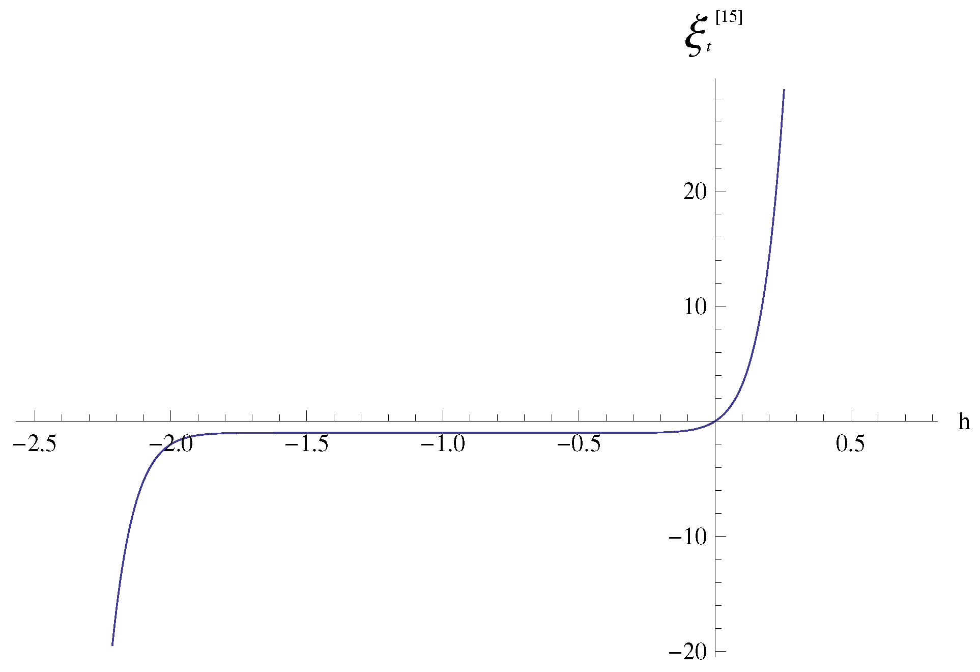
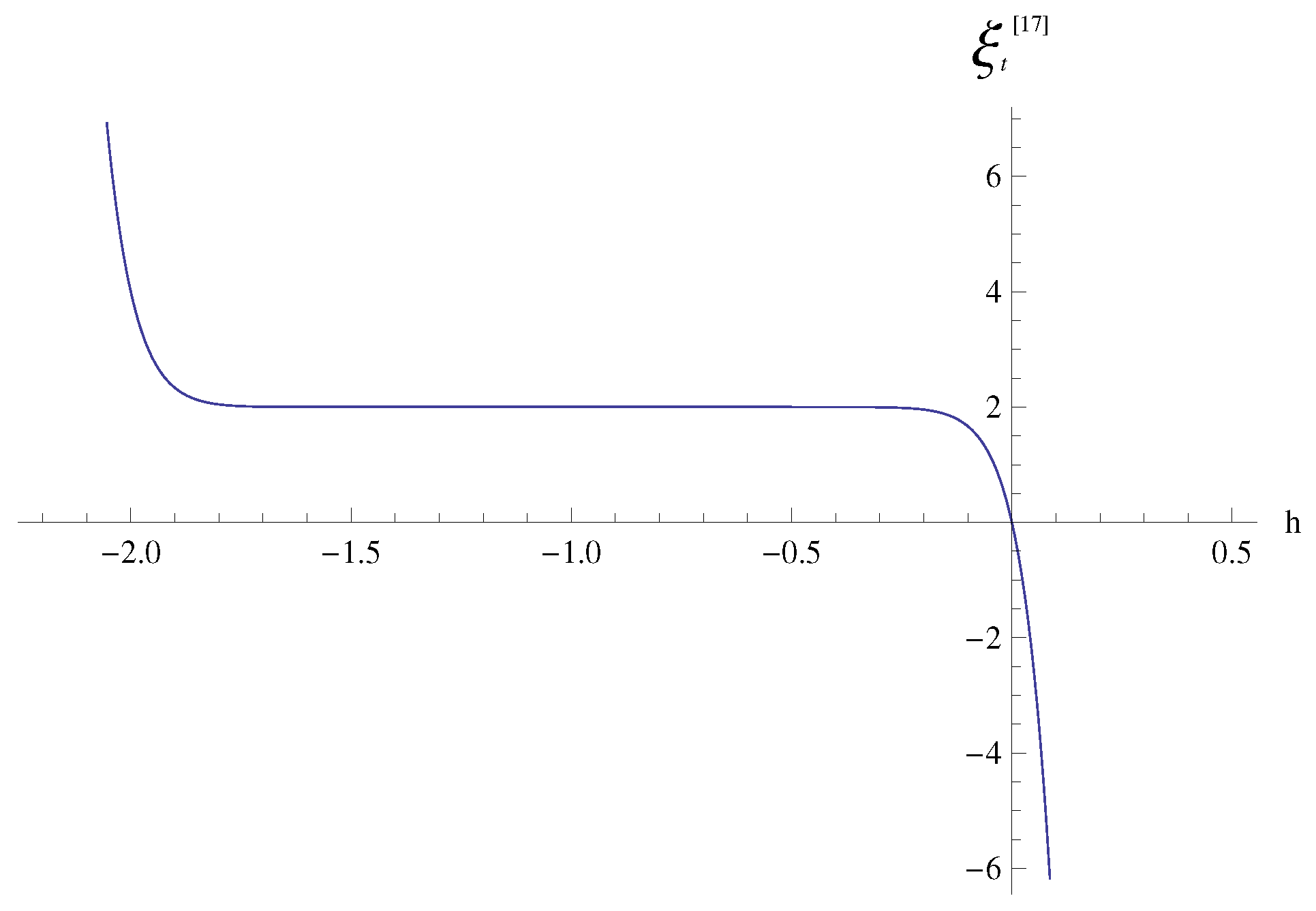
Figure 1 displays the h-curve that corresponds to the 15 t h -order numerical series solution, and this shows that the values of that lead to a convergent series solution are located in the interval ( 2 , 0 ) .
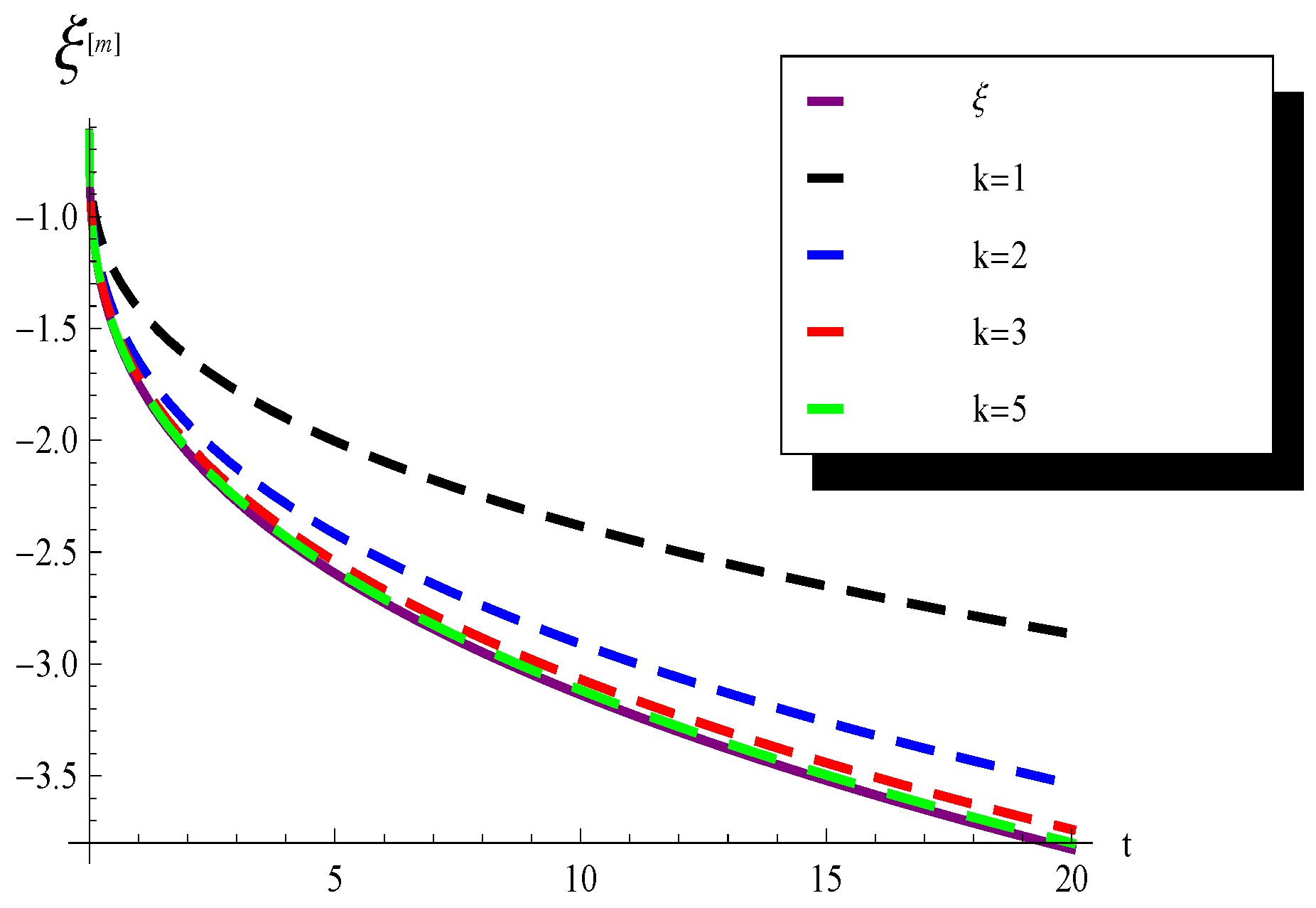
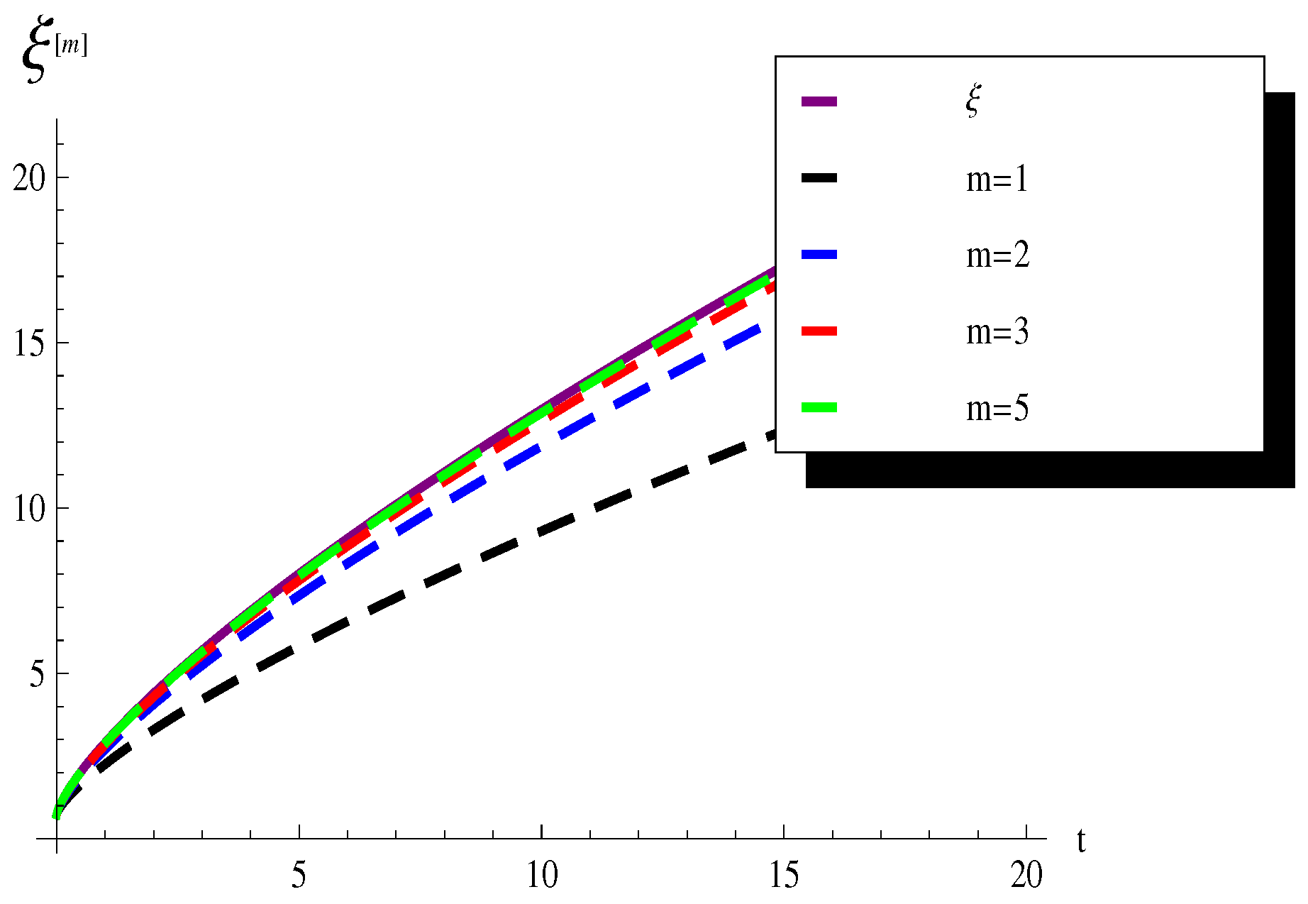
Figure 2 depicts the graphs of the truncated series solution, which used various number of terms together with the corresponding exact solution of Example 1 at x = 0.3 , = 0.7 , and ν = 0.35 . This shows that the truncated series solution of order k = 4 almost coincides with the analytical solution, which indicates the rapid convergence of this method.
In Table 1, Table 2 and Table 3, we present the numerical solutions of Example 1 that result from the k t h -order truncated series solution ξ [ k ] for the many values of k, with = 0.7 at various values of ν , x, and t. As we can see, the results in these tables illustrate the rapid convergences of the generated series solution, which occur just after a few terms.
Table 4 shows the error resulting from the absolute difference | ξ ( x , t ) ξ [ k ] ( x , t ) | of the analytical solution and the numerical truncated series solution of Example 1 for various values of x and t. It illustrates the rapid convergence of the numerical solution that is obtained by utilizing the q-HATM.
Example 2.
Consider the nonhomogeneous fractional-order partial differential equation
t ν ξ 1 x x ξ 2 x 2 ξ = 2 3 x , 0 < ν , x < 1 , 0 < t < T ,
annexed with the following conditions:
ξ ( x , 0 ) = x 3 3 ln ( x ) , 0 < x < 1 , ξ ( 1 , t ) = 1 3 + 2 t ν Γ [ ν + 1 ] , ξ x ( 1 , t ) = 0 , 0 < ν < 1 , 0 < t < T .
Solution.
Here g ( x , t ) = 2 3 x ; hence, it is easy to check that 0 1 x g d x = 0 .
Now, let ξ 0 ( x , t ) = ξ ( x , 0 ) = x 3 3 ln ( x ) . Since n = 1 in view of (10), we obtain the following:
ξ 1 ( x , t ) = χ 1 ξ 0 ( x , t ) + L 1 R ˜ ( ξ 0 ) , = L 1 R ˜ ( ξ 0 ) , = L 1 L { ξ 0 ( x , t ) } ( 1 χ 1 n ) 1 s ξ ( x , 0 ) 1 s ν L { 1 x ( ξ 0 ( x , t ) ) x + ( ξ 0 ( x , t ) ) x x } , = 2 t ν Γ [ ν + 1 ] .
ξ 2 ( x , t ) = χ 2 ξ 1 ( x , t ) + L 1 R ˜ ( ξ 1 ) , = ξ 1 ( x , t ) + L 1 R ˜ ( ξ 1 ) , = ξ 1 ( x , t ) + L 1 L { ξ 1 ( x , t ) } ( 1 χ 2 n ) 1 s ξ ( x , 0 ) 1 s ν L { 1 x ( ξ 1 ( x , t ) ) x + ( ξ 1 ( x , t ) ) x x } , = ( 1 + ) ξ 1 ( x , t ) , = 2 ( 1 + ) t ν Γ [ ν + 1 ] .
ξ 3 ( x , t ) = χ 3 ξ 2 ( x , t ) + L 1 R ˜ ( ξ 2 ) , = ξ 2 ( x , t ) + L 1 R ˜ ( ξ 2 ) , = ξ 2 ( x , t ) + L 1 L { ξ 2 ( x , t ) } ( 1 χ 2 n ) 1 s ξ ( x , 0 ) 1 s ν L { 1 x ( ξ 2 ( x , t ) ) x + ( ξ 2 ( x , t ) ) x x } , = 2 ( 1 + ) 2 t ν Γ [ ν + 1 ] .
If we continue in this manner, we obtain
ξ m ( x , t ) = 2 ( 1 + ) m 1 t ν Γ [ ν + 1 ] ,
hence the following:
ξ ( x , t ) = ξ 0 ( x , t ) + i = 1 ξ j ( x , t ) , = ξ 0 ( x , t ) 2 t ν Γ [ ν + 1 ] ( 1 + ) 2 t ν Γ [ ν + 1 ] ( 1 + ) 2 2 t ν Γ [ ν + 1 ] , = ξ 0 ( x , t ) j = 1 2 ( 1 + ) j 1 t ν Γ [ ν + 1 ] .
Now, if the parameter satisfies 2 < < 0 , then (12) converges, and we obtain the following:
ξ ( x , t ) = ξ 0 ( x , t ) + 2 t ν Γ [ ν + 1 ] , = x 3 3 ln ( x ) + 2 t ν Γ [ ν + 1 ] .
It is clear that at ν = 1 , and the last series converges to the exact solution ξ ( x , t ) = 2 t + x 3 3 ln ( x ) .
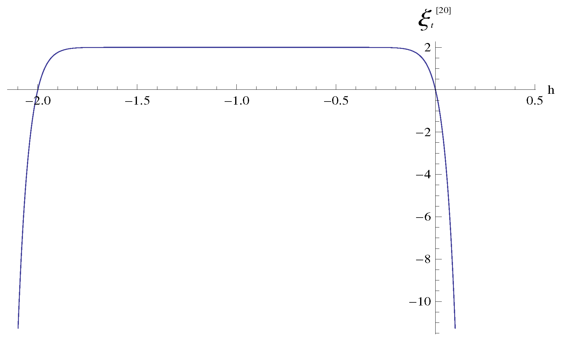
Figure 3 displays the h-curve that corresponds to the 20 t h -order numerical series solution. In addition, it shows that the values of that lead to a convergent series solution are located in the interval ( 2 , 0 ) .
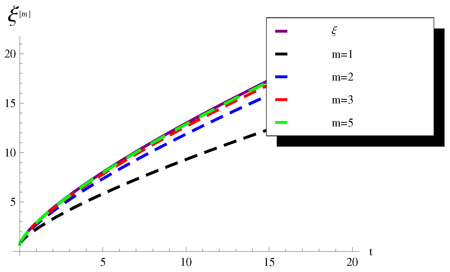
Figure 4 depicts the graphs of the truncated series solution that use various numbers of terms together with the corresponding analytical solution of Example 2 at x = 0.5 , = 0.75 , and ν = 0.35 . This shows that the truncated series solution of order m = 5 almost coincides with the analytical solution, which indicates the rapid convergence of this method.
In Table 5, Table 6 and Table 7, we present the approximate solutions of Example 2 that result from the k t h -order series solution ξ [ k ] for the many values of k,with = 0.7 at various values of ν , x, and t. As we can see, the results in these tables illustrate the rapid convergences of the generated series solutions.
Table 8 shows the error that results from the absolute difference | ξ ( x , t ) ξ [ k ] ( x , t ) | of the analytical solution, as well as the numerical truncated series solution of Example 1 for the various values of x and t. This illustrates the rapid convergence of the numerical solution that results from utilizing the q-HATM.
Example 3.
Consider the nonhomogeneous fractional order partial differential equation:
t ν ξ 1 x x ξ 2 x 2 ξ = 2 1 x , 0 < ν , x < 1 , 0 < t < T ,
annexed with the conditions:
ξ ( x , 0 ) = 1 + x ln ( x ) , 0 < x < 1 , ξ ( 1 , t ) = 1 + x + 2 t ν Γ [ ν + 1 ] , ξ x ( 1 , t ) = 0 , 0 < ν < 1 , 0 < t < T .
Solution.
Here, g ( x , t ) = 2 1 x ; hence, it is easy to see that 0 1 x g d x = 0 .
Next, let ξ 0 ( x , t ) = ξ ( x , 0 ) = 1 + x ln ( x ) . Since n = 1 in view of (10), we obtain the following:
ξ 1 ( x , t ) = χ 1 ξ 0 ( x , t ) + L 1 R ˜ ( ξ 0 ) , = L 1 R ˜ ( ξ 0 ) , = L 1 L { ξ 0 ( x , t ) } ( 1 χ 1 n ) 1 s ξ ( x , 0 ) 1 s ν L { 1 x ( ξ 0 ( x , t ) ) x + ( ξ 0 ( x , t ) ) x x } , = 2 t ν Γ [ ν + 1 ] .
ξ 2 ( x , t ) = χ 2 ξ 1 ( x , t ) + L 1 R ˜ ( ξ 1 ) , = ξ 1 ( x , t ) + L 1 R ˜ ( ξ 1 ) , = ξ 1 ( x , t ) + L 1 L { ξ 1 ( x , t ) } ( 1 χ 2 n ) 1 s ξ ( x , 0 ) 1 s ν L { 1 x ( ξ 1 ( x , t ) ) x + ( ξ 1 ( x , t ) ) x x } , = ( 1 + ) ξ 1 ( x , t ) , = 2 ( 1 + ) t ν Γ [ ν + 1 ] .
ξ 3 ( x , t ) = χ 3 ξ 2 ( x , t ) + L 1 R ˜ ( ξ 2 ) , = ξ 2 ( x , t ) + L 1 R ˜ ( ξ 2 ) , = ξ 2 ( x , t ) + L 1 L { ξ 2 ( x , t ) } ( 1 χ 2 n ) 1 s ξ ( x , 0 ) 1 s ν L { 1 x ( ξ 2 ( x , t ) ) x + ( ξ 2 ( x , t ) ) x x } , = 2 ( 1 + ) 2 t ν Γ [ ν + 1 ] .
If we continue in this way we obtain
ξ m ( x , t ) = 2 ( 1 + ) m 1 t ν Γ [ ν + 1 ] ,
hence
ξ ( x , t ) = ξ 0 ( x , t ) + i = 1 ξ j ( x , t ) , = ξ 0 ( x , t ) 2 t ν Γ [ ν + 1 ] ( 1 + ) 2 t ν Γ [ ν + 1 ] ( 1 + ) 2 2 t ν Γ [ ν + 1 ] , = ξ 0 ( x , t ) j = 1 2 ( 1 + ) j 1 t ν Γ [ ν + 1 ] .
Now, if the parameter satisfies 2 < < 0 , then Series (13) converges, and we obtain the following:
ξ ( x , t ) = ξ 0 ( x , t ) + 2 t ν Γ [ ν + 1 ] , = 1 + x ln ( x ) + 2 t ν Γ [ ν + 1 ] .
It is clear that at ν = 1 , the last series converges to the exact solution ξ ( x , t ) = 2 t + 1 + x ln ( x ) .
Figure 5 displays the h-curve that corresponds to the 17 t h -order numerical series solution. Furthermore, it shows that the values of that lead to a convergent series solution are located in the interval ( 2 , 0 ) .
Figure 6 depicts the graphs of the truncated series solution that use various numbers of terms together with the corresponding exact solution of Example 3 at x = 0.8 , = 0.7 , and ν = 0.6 . This shows that the truncated series solution of order m = 5 almost coincides with the analytical solution, which indicates the rapid convergence of this method.
In Table 9, Table 10 and Table 11, we present the approximate solutions of Example 3 that are produced by an m t h -order series solution ξ [ m ] for many values of m with = 0.7 , which is achieved by using various values of ν , x, and t. As we can see, the results in these tables illustrate the rapid convergences of the generated series solutions.
Table 12 shows the error that results from the absolute difference | ξ ( x , t ) ξ [ k ] ( x , t ) | of the analytical solution, as well as the numerical truncated series solution of Example 1 for various values of x and t. It illustrates the rapid convergence of the numerical solution that results from utilizing the q-HATM.

4. Conclusions

In this article, a numerical solution of a fractional order IBVP with a non-local constraint is obtained via the q-HATM. Several examples are given to illustrate the efficiency of the derived iterative scheme. The exact solution is obtained for each one of these examples. The convergence of the numerical solutions of these examples was studied both numerically and graphically. A comparison of the analytical and numerical solution was conducted using the absolute error for the different values of x and t, as in Table 4, Table 8, and Table 12. Also, a graphical comparison of the truncated series solution with various number of terms and the exact solution is illustrated in Figure 2, Figure 4, and Figure 6. These results show that the q-HATM is an efficient method for solving these types of singular non-local fractional partial differential equations.

Author Contributions

Conceptualization, S.M.; methodology, S.M. and H.A.; software, S.M. and H.A.; validation, S.M. and H.A.; formal analysis, S.M. and H.A.; resources, S.M. and H.A.; investigation, S.M. and H.A. All authors have read and agreed to the published version of the manuscript.

Funding

The authors would like to extend their sincere appreciation to Researchers Supporting Project number (RSP2023R472 King Saud University, Riyadh, Saudi Arabia).

Data Availability Statement

Not applicable.

Acknowledgments

The authors would like to extend their sincere appreciation to Researchers Supporting Project number (RSP2023R472 King Saud University, Riyadh, Saudi Arabia).

Conflicts of Interest

All authors declare no conflict of interest in this paper.

References

  1. Du, M.; Wang, Z.; Hu, H. Measuring memory with the order of fractional derivative. Sci. Rep. 2013, 3, 3431. [Google Scholar]
  2. Scalar, E.; Gorenflo, R.; Mainardi, F. Fractional calculus and continuous time finance. Physica A 2000, 284, 376–384. [Google Scholar]
  3. West, B.J.; Turalskal, M.; Grigolini, P. Fractional calculus ties the microscopic and macroscopic scales of complex network dynamics. New J. Phys. 2015, 17, 45009. [Google Scholar]
  4. Tarasov, V.E. Fractional vector calculus and fractional Maxwell’s equations. Ann. Phys. 2008, 323, 2756–2778. [Google Scholar]
  5. Oldham, K.B.; Spanier, J. The Fractional Calculus; Academic Press: New York, NY, USA, 1974. [Google Scholar]
  6. Miller, K.S.; Ross, B. An Introduction to the Fractional Calculus and Fractional Differential Equations; Willey: New York, NY, USA, 1993. [Google Scholar]
  7. Podlubny, I. Fractional Differential Equations; Academic Press: San Diego, CA, USA, 1999; Volume 198. [Google Scholar]
  8. Kilbas, A.A.; Srivastava, H.M.; Trujillo, J.J. Theory and Applications of Fractional Differential Equations; Elsevier: Amsterdam, The Netherlands, 2006; Volume 204. [Google Scholar]
  9. Baleanu, D.; Diethelm, K.; Scalas, E.; Trujillo, J.J. Fractional Calculus Models and Numerical Methods; World Scientific: Singapore, 2012. [Google Scholar]
  10. Kumar, S. A numerical study for solution of time fractional nonlinear shallow-water equation in oceans. Z. Naturforsch. A 2013, 68, 547–553. [Google Scholar]
  11. Agarwal, R.P.; Benchohra, M.; Hamani, S. A survey on existence results for boundary value problems of nonlinear fractional differential equations and inclusions. Acta Appl. Math. 2010, 109, 973–1033. [Google Scholar]
  12. Kumar, D.; Singh, J.; Kumar, S. Analytical modeling for fractional multi-dimensional diffusion equations by using Laplace transform. Commun. Numer. Anal. 2015, 1, 16–29. [Google Scholar]
  13. Dehghan, M.; Shakeri, F. A semi-numerical technique for solving the multi-point boundary value problems and engineering applications. Int. J. Numer. Methods Heat Fluid Flow 2011, 21, 794–809. [Google Scholar]
  14. Saadatmandi, A.; Dehghan, M. A new operational matrix for solving fractional-order differential equations. Comput. Math. Appl. 2010, 59, 1326–1336. [Google Scholar]
  15. Saadatmandi, A.; Dehghan, M. A tau approach for solution of the space fractional diffusion equation. Comput. Math. Appl. 2011, 62, 1135–1142. [Google Scholar]
  16. Jafari, H.; Golbabai, A.; Seifi, S.; Sayevand, K. Homotopy analysis method for solving multi-term linear and nonlinear diffusion wave equations of fractional order. Comput. Math. Appl. 2010, 66, 838–843. [Google Scholar]
  17. Veeresha, P.; Prakasha1, D.G.; Baskonus, H.M. Novel simulations to the time-fractional Fisher’s equation. Math. Sci. 2019, 13, 33–42. [Google Scholar] [CrossRef]
  18. Mark, M. Meerschaerta and CharlesTadjeran, Finite difference approximations for two-sided space-fractional partial differential equations. Appl. Numer. Math. 2006, 56, 80–90. [Google Scholar]
  19. Jianga, Y.; Ma, J. High-order finite element methods for time-fractional partial differential equations. J. Comput. Appl. Math. 2011, 235, 3285–3290. [Google Scholar] [CrossRef] [Green Version]
  20. Odibata, Z.; Momani, S. The variational iteration method: An efficient scheme for handling fractional partial differential equations in fluid mechanics. Comput. Math. Appl. 2009, 58, 2199–2208. [Google Scholar]
  21. Momani, S.; Odibat, Z. Analytical solution of a time-fractional Navier-Stokes equation by Adomian decomposition method. Appl. Math. Comput. 2006, 177, 488–494. [Google Scholar]
  22. El-Tawil, M.A.; Huseen, S.N. The q-homotopy analysis method (q-HAM). Int. J. Appl. Math. Mech. 2012, 8, 51–75. [Google Scholar]
  23. El-Tawil, M.A.; Huseen, S.N. On convergence of the qhomotopy analysis method. Int. J. Contemp. Math. Sci. 2013, 8, 481–497. [Google Scholar] [CrossRef]
  24. Liao, S.J. The Proposed Homotopy Analysis Technique for the Solution of Nonlinear Problems. Ph.D. Thesis, Shanghai Jiao Tong University, Shanghai, China, 1992. [Google Scholar]
  25. Liao, S.J. Homotopy analysis method a new analytical technique for nonlinear problems. Commun. Nonl. Sci. Numer. Simul. 1997, 2, 95–100. [Google Scholar]
  26. Liao, S.J. Beyond Perturbation: Introduction to the Homotopy Analysis Method; Chapman and Hall/CRC Press: Boca Raton, FL, USA, 2003. [Google Scholar]
  27. Xu, D.L.; Lin, Z.L.; Liao, S.J.; Stiassnie, M. On the steady-state fully resonant progressive waves in water of finite depth. J. Fluid. Mech. 2012, 710, 379–418. [Google Scholar]
  28. Liao, S.J. On the homotopy analysis method for nonlinear problems. Appl. Math. Comput. 2004, 147, 499–513. [Google Scholar]
  29. Prakash, A.; Kaur, H. q-homotopy analysis transform method for space and time-fractional KdV-Burgers equation. Nonlinear Sci. Lett. A 2018, 9, 44–61. [Google Scholar]
  30. Arafa, A.A.M.; Hagag, A.M.S. q-homotopy analysis transform method applied to fractional Kundu-Eckhaus equation and fractional massive Thirring model arising in quantum field theory. Asian-Eur. J. Math. 2019, 12, 1793–5571. [Google Scholar] [CrossRef]
  31. Kumar, D.; Singh, J.; Baleanu, D. A new analysis for fractional model of regularized long-wave equation arising in ion acoustic plasma waves. Math. Methods Appl. Sci. 2017, 40, 5642–5653. [Google Scholar]
  32. Caputo, M. Elasticita e Dissipazione; Zanichelli: Bologna, Italy, 1969. [Google Scholar]
  33. Bagley, R.L.; Torvik, P.J. A theoretical basis for the application of fractional calculus to viscoelasticity. J. Rheol. 1983, 27, 201–210. [Google Scholar]
  34. Sorrentinos, G. Fractional derivative linear models for describing the viscoelastic dynamic behaviorof polymeric beams. In Proceedings of the IMAS, Saint Louis, MO, USA, 30 January–2 February 2006. [Google Scholar]
  35. Mainardi, F. Fractional Calculus and Waves in linear Viscoelasticity: An Introduction to Mathematical Models; World Scientific: Singapore, 2010. [Google Scholar]
  36. Goloviznin, V.M.; Kisilev, V.P.; Korotkin, I.A.; Yurkov, Y.I. Direct Problems of Nonclassical Radionuclide Transfer in Geological Formations. Izv. Ross. Akad. Nauk Energ. 2004, 4, 121–130. [Google Scholar]
  37. Chukbar, K.V. The Stochastic Transfer and Fractional Derivatives. Zh. Eksp. Teor. Fiz. 1995, 108, 1875–1884. [Google Scholar]
  38. Sabatier, J.; Agrawal, O.P.; Machado, J.A.T. (Eds.) Advances in Fractional Calculus: Theoretical Developments and Applications in Physics and Engineering; Springer: Dordrecht, The Netherlands, 2007. [Google Scholar]
  39. Benchohra, M.; Hamani, S.; Ntouyas, S.K. Boundary value problems for differential equations with fractional order and nonlocal conditions. Nonlinear Anal. 2009, 71, 2391–2396. [Google Scholar]
  40. Lazarevic, M.P.; Spasic, A.M. Finite-time stability analysis of fractional order time-delay systems: Gronwall’s approach. Math. Comput. Model. 2009, 49, 475–481. [Google Scholar]
  41. Nieto, J.J. Maximum principles for fractional differential equations derived from Mittag-Leffler functions. Appl. Math. Lett. 2010, 23, 1248–1251. [Google Scholar]
  42. Zhang, S.Q. Positive solutions to singular boundary value problem for nonlinear fractional differential equation. Comput. Math. Appl. 2010, 59, 1300–1309. [Google Scholar]
  43. Mesloub, S.; Obaidat, S. Homotopy Analysis Method for a Fractional Order Equation with Dirichlet and Non-Local Integral Conditions. Mathematics 2019, 7, 1167. [Google Scholar] [CrossRef] [Green Version]
  44. Mesloub, S.; Bachar, I. On a nonlocal 1-D initial value problem for a singular fractional-order parabolic equation with Bessel operator. Adv. Differ. Equ. 2019, 2019, 254. [Google Scholar] [CrossRef]
Figure 1. The -curve that corresponds to the 15 t h -order approximate series solution at x = 0.75 , t = 0 , and ν = 1 .
Axioms 12 00790 g001
Figure 2. Truncated series solution ξ [ k ] ( x , t ) at various values of k together with the analytical solution ξ ( x , t ) of Example 1.
Axioms 12 00790 g002
Figure 3. The -curve that corresponds to the 20 t h -order approximate series solution at x = 0.75 , t = 0 , and ν = 1 .
Axioms 12 00790 g003
Figure 4. The truncated series solution ξ [ m ] ( x , t ) with various values of m together with the analytical solution ξ ( x , t ) of Example 2.
Axioms 12 00790 g004
Figure 5. The -curve that corresponds to the 17 t h -order approximate series solution at x = 0.75 , t = 0 , and ν = 1 .
Axioms 12 00790 g005
Figure 6. Truncated series solution ξ [ m ] ( x , t ) with various values of m together with the exact solution ξ ( x , t ) of Example 3.
Axioms 12 00790 g006
Table 1. The approximate solutions of Example 1 that are generated by ξ [ k ] , and the exact solution ξ at ν = 0.25 and t = 0.1 for certain values of x and k.
x 0.01 0.2 0.5 0.8 0.95
ξ −2.92302−1.43513−1.02948−0.891982−0.871682
k ξ [ k ] ξ [ k ] ξ [ k ] ξ [ k ] ξ [ k ]
1−2.7369−1.24901−0.843361−0.705859−0.685559
2−2.86718−1.37929−0.973647−0.836145−0.815845
3−2.90627−1.41838−1.01273−0.875231−0.854931
13−2.92302−1.43513−1.02948−0.891982−0.871682
100−2.92302−1.43513−1.02948−0.891982−0.871682
200−2.92302−1.43513−1.02948−0.891982−0.871682
Table 2. The numerical solutions of Example 1 that result from ξ [ k ] , and the exact solution ξ , at ν = 0.75 and t = 2 for different values of x and k.
x 0.01 0.2 0.5 0.8 0.95
ξ −4.13251−2.64462−2.23897−2.10147−2.08117
k ξ [ k ] ξ [ k ] ξ [ k ] ξ [ k ] ξ [ k ]
1−3.58354−2.09565−1.69−1.5525−1.5322
2−3.96782−2.47993−2.07428−1.93678−1.91648
3−4.0831−2.59521−2.189572.05206−2.03176
11−4.13251−2.64462−2.23897−2.10147−2.08117
100−4.13251−2.64462−2.23897−2.10147−2.08117
200−4.13251−2.64462−2.23897−2.10147−2.08117
Table 3. The numerical solutions of Example 1 that result from the truncated series ξ [ m ] , and the exact solution ξ , at ν = 0.9 and t = 10 for various values of x and m.
x 0.01 0.2 0.5 0.8 0.95
ξ −10.5617−9.07378−8.66813−8.53063−8.51033
m ξ [ m ] ξ [ m ] ξ [ m ] ξ [ m ] ξ [ m ]
1−8.08395−6.59606−6.19042−6.05291−6.03261
2−9.81836−8.33046−7.92482−7.78732−7.76702
3−10.3387−8.85078−8.44514−8.30764−8.28734
12−10.5617−9.07378−8.66813−8.53063−8.51033
100−10.5617−9.07378−8.66813−8.53063−8.51033
200−10.5617−9.07378−8.66813−8.53063−8.51033
Table 4. The absolute difference between the analytical solution and the numerical solution of the order k of Example 1 at k = 18 , ν = 0.3 , and = 0.7 for various values of x and t.
t
x0.10.2125
0.1 2.16353 × 10 10 3.50633 × 10 10 4.3168 × 10 10 5.31461 × 10 10 6.99606 × 10 10
0.2 2.16353 × 10 10 3.50633 × 10 10 4.3168 × 10 10 5.31461 × 10 10 6.99606 × 10 10
0.5 2.16353 × 10 10 3.50633 × 10 10 4.3168 × 10 10 5.31461 × 10 10 6.99606 × 10 10
0.7 2.16353 × 10 10 3.50633 × 10 10 4.3168 × 10 10 5.31461 × 10 10 6.99606 × 10 10
0.9 2.16353 × 10 10 3.50633 × 10 10 4.3168 × 10 10 5.31461 × 10 10 6.99606 × 10 10
Table 5. The numerical solutions of Example 2 that were obtained using ξ [ k ] , and the exact solution ξ at ν = 0.25 and t = 0.1 for various values of x and k.
x 0.01 0.2 0.5 0.8 0.95
ξ 5.845992.852921.975631.634631.57791
k ξ [ k ] ξ [ k ] ξ [ k ] ξ [ k ] ξ [ k ]
15.473742.480681.603391.262381.20566
25.734322.741251.863961.522961.46623
35.812492.819421.942131.601131.5444
135.845992.852921.975631.634631.57791
1005.845992.852921.975631.634631.57791
2005.845992.852921.975631.634631.57791
Table 6. The approximate solutions of Example 2 that were generated by ξ [ k ] , and the exact solution ξ at ν = 0.75 and t = 2 for different values of x and k.
x 0.01 0.2 0.5 0.8 0.95
ξ 8.264975.271914.394614.053613.99689
k ξ [ k ] ξ [ k ] ξ [ k ] ξ [ k ] ξ [ k ]
17.167034.173973.296672.955672.89895
27.935594.942524.065233.724233.6675
38.166165.173094.29583.95483.89807
138.264975.27194.394614.053613.99689
1008.264975.271914.394614.053613.99689
2008.264975.271914.394614.053613.99689
Table 7. The numerical solutions of Example 2 that were produced by ξ [ m ] , and the exact solution ξ at ν = 0.9 and t = 10 for various values of x and m.
x 0.01 0.2 0.5 0.8 0.95
ξ 21.123318.130217.252916.911916.8552
m ξ [ m ] ξ [ m ] ξ [ m ] ξ [ m ] ξ [ m ]
116.167900012.297511.956511.8998
219.636716.643615.766315.425315.3686
320.677317.684216.806916.465916.4092
1121.123318.130217.252916.911916.8552
10021.123318.130217.252916.911916.8552
20021.123318.130217.252916.911916.8552
Table 8. The absolute difference between the analytical solution and the truncated series solution of order k of Example 2 at k = 18 , ν = 0.6 , and = 0.7 for various values of x and t.
t
x0.10.2125
0.1 2.17826 × 10 10 5.72127 × 10 10 8.67183 × 10 10 1.3144 × 10 9 2.27768 × 10 9
0.2 2.17827 × 10 10 5.72126 × 10 10 8.67183 × 10 10 1.3144 × 10 9 2.27768 × 10 9
0.5 2.17826 × 10 10 5.72127 × 10 10 8.67182 × 10 10 1.3144 × 10 9 2.27768 × 10 9
0.7 2.17826 × 10 10 5.72127 × 10 10 8.67182 × 10 10 1.3144 × 10 9 2.27768 × 10 9
0.9 2.17827 × 10 10 5.72127 × 10 10 8.67182 × 10 10 1.3144 × 10 9 2.27768 × 10 9
Table 9. The approximate solutions of Example 3 that were generated by ξ [ m ] , and the exact solution ξ at ν = 0.25 and t = 0.1 for various values of x and m.
x 0.01 0.2 0.5 0.8 0.95
ξ 6.855994.050263.433973.263963.24211
m ξ [ m ] ξ [ m ] ξ [ m ] ξ [ m ] ξ [ m ]
16.483743.678013.061722.891722.86987
26.744323.938583.322293.152293.13044
36.822494.016763.400473.230463.20861
116.855994.050263.433973.263963.24211
1006.855994.050263.433973.263963.24211
2006.855994.050263.433973.263963.24211
Table 10. The approximate solutions of Example 3 that are generated by ξ [ m ] , and the exact solution ξ , at ν = 0.75 and t = 2 for various values of x and m.
x 0.01 0.2 0.5 0.8 0.95
ξ 9.274976.469245.852955.682945.66109
m ξ [ m ] ξ [ m ] ξ [ m ] ξ [ m ] ξ [ m ]
18.177035.37134.755014.5854.56315
28.945596.139865.523575.353565.33171
39.176166.370425.754135.584135.56228
129.274976.469245.852955.682945.66109
1009.274976.469245.852955.682945.66109
2009.274976.469245.852955.682945.66109
Table 11. The approximate solutions of Example 3 that are generated by ξ [ m ] , and the exact solution ξ at ν = 0.9 and t = 10 for various values of x and m.
x 0.01 0.2 0.5 0.8 0.95
ξ 22.133319.327618.711318.541318.5194
m ξ [ m ] ξ [ m ] ξ [ m ] ξ [ m ] ξ [ m ]
117.177914.372113.755813.585813.564
220.646717.840917.224617.054617.0328
321.687318.881618.265318.095318.0734
1222.133319.327618.711318.541318.5194
10022.133319.327618.711318.541318.5194
20022.133319.327618.711318.541318.5194
Table 12. The absolute difference between the analytical solution and the truncated series solution of order k of Example 3 at k = 19 , ν = 0.75 , and = 0.7 for various values of x and t.
t
x0.10.2125
0.1 4.49769 × 10 11 1.5039 × 10 10 2.52923 × 10 10 4.25363 × 10 10 8.457 × 10 10
0.2 4.49769 × 10 11 1.5039 × 10 10 2.52923 × 10 10 4.25365 × 10 10 8.45699 × 10 10
0.5 4.49765 × 10 11 1.50389 × 10 10 2.52924 × 10 10 4.25364 × 10 10 8.45699 × 10 10
0.7 4.49769 × 10 11 1.50389 × 10 10 2.52923 × 10 10 4.25365 × 10 10 8.457 × 10 10
0.9 4.49769 × 10 11 1.50389 × 10 10 2.52922 × 10 10 4.25364 × 10 10 8.45699 × 10 10
Disclaimer/Publisher’s Note: The statements, opinions and data contained in all publications are solely those of the individual author(s) and contributor(s) and not of MDPI and/or the editor(s). MDPI and/or the editor(s) disclaim responsibility for any injury to people or property resulting from any ideas, methods, instructions or products referred to in the content.

