Article

An Analytic Solution for 2D Heat Conduction Problems with Space–Time-Dependent Dirichlet Boundary Conditions and Heat Sources

1
Department of Aircraft Engineering, Air Force Institute of Technology, 1 Associate Jyulun Road, Gang-Shan District, Kaoshiung City 820, Taiwan
2
Department of Mechanical Engineering, Air Force Institute of Technology, 1 Associate Jyulun Road, Gang-Shan District, Kaoshiung City 820, Taiwan
3
Department of Aircraft Maintenance, Far East University, 49 Zhonghua Road, Xinshi District, Tainan City 744, Taiwan
*
Author to whom correspondence should be addressed.
Axioms 2023, 12(7), 708; https://doi.org/10.3390/axioms12070708
Submission received: 20 June 2023 / Revised: 18 July 2023 / Accepted: 19 July 2023 / Published: 20 July 2023
(This article belongs to the Special Issue Applied Mathematics in Energy and Mechanical Engineering)

Abstract

:
This study proposes a closed-form solution for the two-dimensional (2D) transient heat conduction in a rectangular cross-section of an infinite bar with space–time-dependent Dirichlet boundary conditions and heat sources. The main purpose of this study is to eliminate the limitations of the previous study and add heat sources to the heat conduction system. The restriction of the previous study is that the values of the boundary conditions and initial conditions at the four corners of the rectangular region should be zero. First, the boundary value problem of 2D heat conduction system is transformed into a dimensionless form. Second, the dimensionless temperature function is transformed so that the temperatures at the four endpoints of the boundary of the rectangular region become zero. Dividing the system into two one-dimensional (1D) subsystems and solving them by combining the proposed shifting function method with the eigenfunction expansion theorem, the complete solution in series form is obtained through the superposition of the subsystem solutions. Three examples are studied to illustrate the efficiency and reliability of the method. For convenience, the space–time-dependent functions used in the examples are considered separable in the space–time domain. The linear, parabolic, and sine functions are chosen as the space-dependent functions, and the sine, cosine, and exponential functions are chosen as the time-dependent functions. The solutions in the literature are used to verify the correctness of the solutions derived using the proposed method, and the results are completely consistent. The parameter influence of the time-dependent function of the boundary conditions and heat sources on the temperature variation is also investigated. The time-dependent function includes exponential type and harmonic type. For the exponential time-dependent function, a smaller decay constant of the time-dependent function leads to a greater temperature drop. For the harmonic time-dependent function, a higher frequency of the time-dependent function leads to a more frequent fluctuation of the temperature change.

1. Introduction

Heat conduction problems commonly exist in various modern mechanical equipment and advanced instruments, and the boundary conditions and the heat sources of these heat conduction problems are often space–time-dependent. Over the years, much research has been devoted to these problems. The main methods to solve these problems include numerical methods, analytic methods, and experimental methods. The literature review below focuses on the study of heat conduction problems with time- and/or space-dependent boundary conditions and/or heat sources.
Some advanced books on heat conduction described some classical techniques for solving heat conduction problems [1,2,3]. These include Laplace transform, Green’s function, and Duhamel’s theorem. Different approximation methods have been used to study one-dimensional (1D) heat conduction problems with space- and/or time-dependent boundary conditions and heat sources, such as the iterative perturbation method used by Holy [4] and the eigenfunction expansion method used by Özisik and Murray [5]. Johansson and Lesnic [6], Chantasiriwan [7], and Young et al. [8] applied the fundamental solutions method to the time-dependent heat conduction problems. On the basis of the boundary element method, Zhu, Liu, and Lu [9] used the Laplace transform, and Bulgakov, Sarler, and Kuhn [10] used the finite difference scheme to find the solution in the time domain. Lee et al. [11] proposed an integration-free-solution method to derive the analytic closed solution to the one-dimensional heat conduction problem with time-dependent boundary conditions. Furthermore, they extended the solution method and successfully applied it to the inverse analysis of heat conduction problems [12,13].
Several numerical techniques have been proposed for two- and three-dimensional (2D and 3D) heat conduction problems with space- and/or time-dependent boundary conditions and/or heat sources. Walker [14] applied the fundamental solution of diffusion combined with time integration to solve the diffusion equation. Chen, Golberg, and Hon [15] applied the modified Helmholtz fundamental solution to the diffusion equation. Zhu [16] and Sutradhar, Paulino, and Gray [17] used the Laplace transform to deal with the time derivative term in the diffusion equation. Burgess and Mahajerin [18] used the fundamental collocation method to the problems of arbitrary shapes subjected to mixed time-dependent boundary conditions and arbitrary initial conditions. Young, Tsai, and Fan [19] solved the nonhomogeneous diffusion problems using the fundamental solution method and the dual reciprocity method. Numerical computation using the Padé scheme was proposed by Siddique [20] to solve two-dimensional diffusion problems. The finite integral transform method was used by Singh et al. [21] to solve the problem of asymmetric heat conduction in a multilayer annulus space with time-dependent boundary conditions and/or heat sources. Hematiyan et al. [22] presented a boundary element method to analyze the 2D and 3D uncoupled thermoelastic problems with space- and time-dependent heat sources. An enhanced state-space method considering laminate approximation theory was introduced by Daneshjou et al. [23] to analyze the non-Fourier heat conduction of an infinite 2D functionally graded hollow cylinder influenced by a time-dependent heat source.
Gu et al. [24] proposed the generalized finite difference method to recover the time-dependent heat sources associated with a 3D heat equation. The eigenfunction-based solutions of various heat conduction models exhibited a mismatch at the boundaries. Biswas et al. [25] homogenized the generalized time-dependent boundary conditions to remove this mismatch from the solution. Akbari et al. [26] employed Duhamel’s theorem to evaluate the non-Fourier heat conduction of the 3D hollow spheres under the space- and time-dependent boundary conditions. Zhou et al. [27] proposed a polygonal boundary element method to solve the nonlinear heat conduction problems with space-dependent heat source and temperature-dependent thermal properties. The authors [28] derived a closed-form solution to the 2D heat conduction problem with the general Dirichlet boundary condition using the shifting function method with the eigenfunction expansion theorem. However, the temperature values of the boundary conditions and initial condition at the four corners of the rectangular region were restricted to zero, which limited the applicability of this study. Moreover, no heat source was considered in this document.
In this paper, a closed solution to the transient heat conduction problems in a rectangular cross-section of an infinite bar with nonhomogeneous space–time-dependent Dirichlet boundary conditions and heat sources was developed. This study addresses the limitations of the previous study [28]; that is, the values of the boundary conditions and initial conditions at the four corners of the rectangular area do not need to be limited to zero and become functions of time. The space–time-dependent heat sources are also considered in this study. The scope of application becomes much larger. This solution has a wide range of applications, such as laser heating, living tissue research, electronic devices, and microstructural applications [12,25,29,30]. The proposed method can accurately solve the heat conduction problem modeled as a rectangular cross-section of an infinite bar with Dirichlet boundary conditions and heat sources. The first step in solving the two-dimensional heat conduction problem is to change the physic system to be a dimensionless form. Afterward, the temperature function is transformed so that the temperature values at the four endpoints of the boundary conditions of the rectangular region become zero. Then, the system is divided into two separate one-dimensional subsystems. The governing differential equations with nonhomogeneous space- and time-dependent boundary conditions are transformed into differential equations with homogeneous boundary conditions by applying the shifting function method which does not require any integral transformation. Under the transformed homogeneous boundary conditions, the closed-form solution of the system can be further deduced by using the eigenfunction expansion theorem. Combining the solutions of the two individual subsystems, the analytic solution of the original two-dimensional heat conduction system can be obtained. Three examples are employed to illustrate the efficiency and reliability of the method. The solution obtained using the proposed method is in full agreement with the literature. The influence of the parameters is also investigated.
The contributions of this paper are as follows:
(1)
The analytic solution to 2D heat conduction problems with the general Dirichlet boundary conditions using the shifting function method with the expansion theorem method was proposed in our previous study [28]. However, there were two restrictions, the temperature values at the four corners of the rectangular area should be zero, and the heat source was also set to zero. The greatest contribution of this work is that an analytical solution is proposed first for the 2D transient heat conduction in a rectangular cross-section of an infinite bar with the space–time-dependent Dirichlet boundary conditions and heat sources. The temperatures at the four corners of the rectangular region can be functions of time.
(2)
The correctness of the solution in this study is verified by comparing the solutions of some cases using the proposed method with those of Young et al. [8], the previous work [28], and Siddique [20]. To the best of the authors’ knowledge, the other cases in this paper have never been presented in past studies. Furthermore, the case studies show that the proposed method has good convergence to the solution using series expansion and can quickly reach the converged value. The parameter influence of the time-dependent function of the boundary conditions and heat sources on the temperature change is also studied.

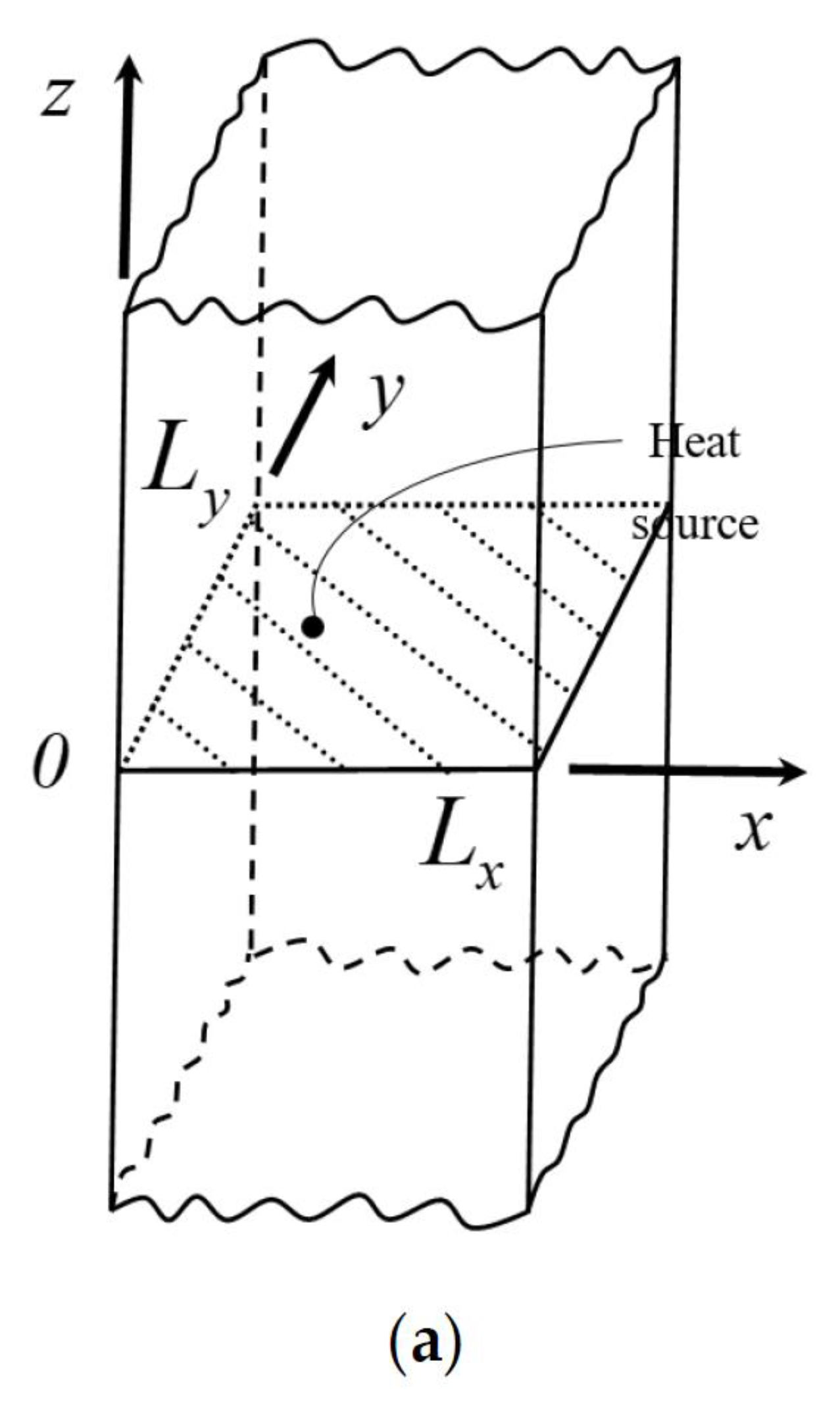
2. Mathematical Modeling and Dimensionless Form of Physical System

Consider the transient heat conduction for a rectangular cross-section in an infinite bar with the space–time-dependent Dirichlet boundary conditions on its four sides and the heat generation inside the bar. The material of the bar is isotropic and time-independent, implying that the material properties are constants. Figure 1 shows the geometry, heat sources, boundary conditions, and initial conditions of a rectangular cross-section in an infinite bar. Therefore, the governing equation, boundary conditions, and initial conditions of the physical system are given as follows:
k 2 T ( x , y , t ) x 2 + 2 T ( x , y , t ) y 2 + g ( x , y , t ) = ρ c T ( x , y , t ) t   in   0 x L x ,   0 y L y ,   t > 0 ,
T ( 0 , y , t ) = f 1 ( y , t ) ,   at   x = 0 ,   0 y L y ,
T ( L x , y , t ) = f 2 ( y , t ) ,   at   x = L x ,   0 y L y ,
T ( x , 0 , t ) = f 3 ( x , t ) ,   at   y = 0 ,   0 x L x ,
T ( x , L y , t ) = f 4 ( x , t ) ,   at   y = L y ,   0 x L x ,
T ( x , y , 0 ) = T 0 ( x , y ) ,   at   t = 0 ,   0 x L x ,   0 y L y ,
where T ( x , y , t ) is the temperature function, g ( x , y , t ) denotes the heat source inside the rectangular cross-section, x and y are the two-dimensional space variables, L x and L y are the thickness of the rectangular bar in the x - and y -directions, respectively, and t is the time variable. In addition, k , ρ , and c represent the thermal conductivity, mass density, and specific heat, respectively. f i ( y , t ) i = 1 , 2 and f i ( x , t ) i = 3 , 4 represent the general case of space–time-dependent temperatures prescribed along the surfaces at the left and right sides and at the bottom and top sides, respectively. It is worth noting that the heat source function g ( x , y , t ) in Equation (1) is a function of space variables, which means that there are infinitely many heat sources allowed in this function. If multiple heat source functions are required to model the heat sources, the function g ( x , y , t ) in Equation (1) can be changed to a summation term of these functions. The matching boundary conditions to initial conditions have the following properties:
f 1 ( y ,   0 ) = T 0 ( 0 ,   y ) ,   f 2 ( y , 0 ) = T 0 ( L x , y ) ,   f 3 ( x , 0 ) = T 0 ( x , 0 ) ,   f 4 ( x , 0 ) = T 0 ( x , L y ) .
For ease of discussion, a dimensionless form of the 2D heat conduction system is first generated. After introducing the dimensionless parameters
ψ ( X , Y , τ ) = T ( x , y , t ) T r ,   G ¯ ( X , Y , τ ) = L y 2   g ( x , y , t ) k T r ,   τ = α   t L y 2 ,   X = x L x ,   Y = y L y ,   L r = L y L x , F ¯ i ( Y , τ ) = f i ( y , t ) T r ,   i = 1 , 2 ,   F ¯ i ( X , τ ) = f i ( x , t ) T r ,   i = 3 , 4 ,   ψ 0 ( X , Y ) = T 0 ( x , y ) T r ,
the dimensionless form of the boundary value problem becomes
L r 2 2 ψ ( X , Y , τ ) X 2 + 2 ψ ( X , Y , τ ) Y 2 + G ¯ ( X , Y , τ ) = ψ ( X , Y , τ ) τ ,   in   0 < X < 1 , 0 < Y < 1 ,   τ > 0 ,
ψ ( 0 , Y , τ ) = F ¯ 1 ( Y , τ ) ,   ψ ( 1 , Y , τ ) = F ¯ 2 ( Y , τ ) ,   ψ ( X , 0 , τ ) = F ¯ 3 ( X , τ ) ,   ψ ( X , 1 , τ ) = F ¯ 4 ( X , τ ) ,
ψ ( X , Y , 0 ) = ψ 0 ( X , Y ) .
The parameter α = k ρ   c in Equation (8) represents the thermal diffusivity, and T r represents the reference temperature. The matching conditions of the boundary conditions and the initial conditions also become
F ¯ 1 ( Y ,   0 ) = ψ 0 ( 0 ,   Y ) ,   F ¯ 2 ( Y , 0 ) = ψ 0 ( 1 , Y ) ,   F ¯ 3 ( X , 0 ) = ψ 0 ( X , 0 ) ,   F ¯ 4 ( X , 0 ) = ψ 0 ( X , 1 ) .

3. The Solution Method

The previous study [28] presented a method to derive an analytic solution to a 2D heat conduction problem with general Dirichlet boundary conditions. However, the heat generation was not considered in the model. Moreover, the values of boundary conditions and initial conditions at each endpoint of the rectangular area were limited to zero, which limited the applicability of this method. In this study, the constraint of corner zeros of the boundary conditions was removed by first variable-transforming the temperature, and the space–time-dependent heat source was added to the heat conduction system. The system was then divided into two subsystems, each of which can be solved with a 1D heat conduction problem. By properly choosing the shifting function, the second-order governing differential equation with space–time-dependent boundary conditions was transformed into a differential equation with homogeneous boundary conditions. Due to the homogeneous boundary conditions, the eigenfunction expansion theorem could be applied to solve the closed-form solution of the subsystem. Lastly, the solutions of the two subsystems were added to obtain the analytic solution for 2D heat conduction in a rectangular region with space–time Dirichlet boundary conditions and heat sources

3.1. Temperature Variable Transformation

a ( τ ) , b ( τ ) , c ( τ ) , and d ( τ ) represent the temperature at each endpoint of the rectangular section (Figure 2a) and can be expressed as follows.
a ( τ ) = F ¯ 1 ( 0 ,   τ ) = F ¯ 3 ( 0 ,   τ ) ,   b ( τ ) = F ¯ 2 ( 0 ,   τ ) = F ¯ 3 ( 1 ,   τ ) ,   c ( τ ) = F ¯ 1 ( 1 ,   τ ) = F ¯ 4 ( 0 ,   τ ) ,   d ( τ ) = F ¯ 2 ( 1 ,   τ ) = F ¯ 4 ( 1 ,   τ ) .
To increase the method applicability of our previous study [28], the nonzero temperatures at the four endpoints can be converted to zero first (Figure 2b). Therefore, variable transformation to achieve this goal can be expressed as follows:
θ ( X , Y , τ ) = ψ ( X , Y , τ ) a ( τ ) + X   [ b ( τ ) a ( τ ) ] + Y   [ c ( τ ) a ( τ ) + X   Y   ( d ( τ ) c ( τ ) b ( τ ) + a ( τ ) ) ] .
Substituting Equation (14) back into Equation (9) can obtain the following nonhomogeneous differential equation:
L r 2 2 θ ( X , Y , τ ) X 2 + 2 θ ( X , Y , τ ) Y 2 + G ( X , Y , τ ) = θ ( X , Y , τ ) τ ,   in   0 < X < 1 , 0 < Y < 1 ,   τ > 0 ,
where the transformed dimensionless heat source G ( X , Y , τ ) is defined as
G ( X , Y , τ ) = G ¯ ( X , Y , τ ) ρ c a ˙ ( τ ) + X   [ b ˙ ( τ ) a ˙ ( τ ) ] + Y   [ c ˙ ( τ ) a ˙ ( τ ) + X   Y   [ d ˙ ( τ ) c ˙ ( τ ) b ˙ ( τ ) + a ˙ ( τ ) ] ,
and the dot is used to indicate the differentiation with respect to the dimensionless time τ .
The dimensionless boundary conditions and initial conditions become
θ ( 0 , Y , τ ) = F 1 ( Y , τ ) = F ¯ 1 ( Y , τ ) a ( τ ) + Y   [ c ( τ ) a ( τ ) ] ,   at   X = 0 ,   0 Y 1 ,
θ ( 1 , Y , τ ) = F 2 ( Y , τ ) = F ¯ 2 ( Y , τ ) b ( τ ) + Y   [ d ( τ ) b ( τ ) ] ,   at   X = 1 ,   0 Y 1 ,
θ ( X , 0 , τ ) = F 3 ( X , τ ) = F ¯ 3 ( X , τ ) a ( τ ) + X   [ b ( τ ) a ( τ ) ] ,   at   Y = 0 ,   0 X 1 ,
θ ( X , 1 , τ ) = F 4 ( X , τ ) = F ¯ 4 ( X , τ ) c ( τ ) + X   [ d ( τ ) c ( τ ) ] ,   at   Y = 1 ,   0 X 1 ,
θ ( X , Y , τ ) = θ 0 ( X , Y ) = ψ 0 ( X , Y ) a ( 0 ) + X   [ b ( 0 ) a ( 0 ) ] + Y   [ c ( 0 ) a ( 0 ) ] + X   Y   [ d ( 0 ) c ( 0 ) b ( 0 ) + a ( 0 ) ] ,                                                                                                                                                                                                                                               at   τ = 0 ,   0 X 1 ,   0 Y 1 .
In addition, considering the compatibility of the boundary conditions and initial conditions, we have
F 1 ( Y , 0 ) = θ 0 ( 0 , Y ) ,   F 2 ( Y , 0 ) = θ 0 ( 1 , Y ) ,   F 3 ( X , 0 ) = θ 0 ( X , 0 ) ,   F 4 ( X , 0 ) = θ 0 ( X , 1 ) .

3.2. Principle of Superposition

Due to the boundary value problem with the linear characteristic, we can divide the physical system into two subsystems A and B in the X - and Y -directions through the principle of superposition, as shown in Figure 3.
θ ( X , Y , τ ) is spilt into two branches as follows:
θ ( X , Y , τ ) = θ a ( X , Y , τ ) + θ b ( X , Y , τ ) .
For subsystem A , the governing equation, and the boundary and initial conditions of the heat conduction problem are
L r 2 2 θ a ( X , Y , τ ) X 2 + 2 θ a ( X , Y , τ ) Y 2 + G a ( X , Y , τ ) = θ a ( X , Y , τ ) τ ,   in   0 X 1 ,   0 Y 1 , τ > 0 ,
θ a ( 0 , Y , τ ) = F 1 ( Y , τ ) ,   θ a ( 1 , Y , τ ) = F 2 ( Y , τ ) ,   θ a ( X , 0 , τ ) = 0 ,   θ a ( X , 1 , τ ) = 0 ,
θ a ( X , Y , 0 ) = θ a 0 ( X , Y ) ,   at   τ = 0 ,   0 X 1 ,   0 Y 1 .
Similarly, for subsystem B , the governing equation, and the boundary and initial conditions of the heat conduction problem are
L r 2 2 θ b ( X , Y , τ ) X 2 + 2 θ b ( X , Y , τ ) Y 2 + G b ( X , Y , τ ) = θ b ( X , Y , τ ) τ ,   in   0 X 1 ,   0 Y 1 , τ > 0 ,
θ b ( 0 , Y , τ ) = 0 ,   θ b ( 1 , Y , τ ) = 0 ,   θ b ( X , 0 , τ ) = F 3 ( X , τ ) ,   θ b ( X , 1 , τ ) = F 4 ( X , τ ) ,
θ b ( X , Y , 0 ) = θ 0 ( X , Y ) θ a 0 ( X , Y ) = θ b 0 ( X , Y ) .
Considering the similarity of the two subsystems, for the sake of brevity, subsystem A is solved first, while subsystem B is solved in Appendix A.

3.3. Reduction to One-Dimensional Problem

Considering two homogeneous boundary conditions on opposite sides of a rectangular cross-section, namely, Y = 0 and Y = 1 , it is reasonable to assume that the temperature θ a ( X , Y , τ ) , the heat source G a ( X , Y , τ ) , and the dimensionless boundary values F i ( Y , τ ) ( i = 1 , 2 ) defined in Equations (24) and (25) become
θ a ( X , Y , τ ) = m = 1 θ m ( X , τ ) sin ( m π Y ) ,
G a ( X , Y , τ ) = m = 1 G a m ( X , τ ) sin ( m π Y ) ,
F i ( Y , τ ) = m = 1 F ¯ i , m ( τ ) sin ( m π Y ) ,   i = 1 , 2 ,
where G a m ( X , τ ) and F ¯ i , m ( τ ) ( i = 1 , 2 ) , are defined as
G a m ( X , τ ) = 2 0 1 G a ( X , Y , τ ) sin ( m π Y )   d Y ,
F ¯ i , m ( τ ) = 2 0 1 F i ( Y , τ ) sin ( m π Y ) d Y ,   i = 1 , 2 .
θ m ( X , τ ) in Equation (30) is determined by meeting the governing equation and the boundary conditions on both edges X = 0 and X = 1 (the first two terms in Equation (25)). Substituting Equations (30)–(32) into Equations (24)–(26) yields the following result:
θ m X , τ τ L r 2 2 θ m X , τ X 2 + m 2 π 2 θ m X , τ = G a m ( X , τ ) ,   in   0 < X < 1 ,   τ > 0 ,
θ m ( 0 , τ ) = F ¯ 1 , m ( τ ) ,   θ m ( 1 , τ ) = F ¯ 2 , m ( τ ) ,
θ m ( X , 0 ) = 2 0 1 θ a 0 ( X , Y ) sin ( m π Y ) d Y .

3.4. The Shifting Function Method

3.4.1. Change of Variable

To find the solution of the second-order partial differential Equation (35) with nonhomogeneous boundary conditions (Equation (36)), the following transformation equation can be employed to extend the shifting function method [11,12,13]:
θ m ( X , τ ) = θ ¯ m ( X , τ ) + i = 1 2 [ g i , m ( X ) F ¯ i , m ( τ ) ] ,
where θ ¯ m ( X , τ ) is the transformed function, and g i , m ( X ) ( i = 1 , 2 ) are the two shifting functions to be determined.
Substituting Equation (38) into Equations (35)–(37) yields
θ ¯ ˙ m ( X , τ ) + i = 1 2 [ g i , m ( X ) F ¯ ˙ i , m ( τ ) ] L r 2 θ ¯ m ( X , τ ) + i = 1 2 [ g i , m ( X ) F ¯ i , m ( τ ) ] + m 2 π 2 θ ¯ m ( X , τ ) + i = 1 2 [ g i , m ( X ) F ¯ i , m ( τ ) ] = G a m ( X , τ ) ,
where the double primes are used to denote twice differentiation with respect to dimensionless coordinate X . The associated boundary conditions become
θ ¯ m ( 0 , τ ) + i = 1 2 [ g i , m ( 0 ) F ¯ i , m ( τ ) ] = F ¯ 1 , m ( τ ) ,   θ ¯ m ( 1 , τ ) + i = 1 2 [ g i , m ( 1 ) F ¯ i , m ( τ ) ] = F ¯ 2 , m ( τ ) .

3.4.2. The Shifting Functions

For the convenience of subsequent analysis, the shifting functions can be chosen to satisfy the following differential equation and boundary conditions:
g i , m ( X ) = 0 ,   i = 1 , 2 ,   0 < X < 1 ,
g i , m ( 0 ) = δ i 1 ,   g i , m ( 1 ) = δ i 2 ,
where δ i j is the Kronecker delta. Two shifting functions are, thus, easily specified as
g 1 , m ( X ) = 1 X ,   g 2 , m ( X ) = X .
Substituting Equations (41)–(43) into Equations (39) and (40), the differential equation for θ ¯ m ( X , τ ) is simplified as follows:
θ ¯ ˙ m ( X , τ ) L r 2 θ ¯ m ( X , τ ) + m 2 π 2 θ ¯ m ( X , τ ) = G ¯ m ( X , τ ) ,
and the homogeneous boundary conditions are
θ ¯ m ( 0 , τ ) = 0 ,   θ ¯ m ( 1 , τ ) = 0 .
G ¯ m ( X , τ ) in Equation (44) is defined as
G ¯ m ( X , τ ) = i = 1 2 g i , m ( X ) [ F ¯ ˙ i , m ( τ ) + m 2 π 2 F ¯ i , m ( τ ) ] + G a m ( X , τ ) .
In addition, the initial condition is transformed to be
θ ¯ m ( X , 0 ) = 2 0 1 θ a 0 ( X , Y ) sin ( m π Y ) d Y i = 1 2 [ g i , m ( X ) F ¯ i , m ( 0 ) ] .

3.4.3. The Series Expansion Theorem

The solution θ ¯ m ( X , τ ) of Equations (44) and (45) can be solved by applying the method of separation variable. In this method, the solution θ ¯ m ( X , τ ) is expressed as
θ ¯ m ( X , τ ) = n = 1 [ θ ¯ m n ( X )   T m n a ( τ ) ] ,
where the space variable θ ¯ m n ( X ) is solved by the following Sturm–Liouville eigenvalue problem:
θ ¯ m n ( X ) + ω n 2 θ ¯ m n ( X ) = 0 ,   0 < X < 1 ,
θ ¯ m n ( 0 ) = 0 ,   θ ¯ m n ( 1 ) = 0 .
The eigenfunctions θ ¯ m n ( X ) ( n = 1 ,   2 ,   3 , ) . and the corresponding eigenvalues are solved as
θ ¯ m n ( X ) = sin ω n X ,   ω n = n π ,   n = 1 ,   2 ,   3 ,  
The eigenfunctions constitute an orthogonal set in the interval [ 0 ,   1 ] ,
0 1 θ ¯ m i ( X )   θ ¯ m j ( X ) d X = 0 for i j 1 2 for i = j .
Substituting Equation (51) into Equation (48), substituting Equation (48) into Equation (44), multiplying Equation (44) by θ ¯ m n ( X ) , and integrating from 0 to 1, the following differential equation can be obtained:
T ˙ m n a ( τ ) + λ m n a 2 T m n a ( τ ) = γ m n a ( τ ) ,
where λ m n a and γ m n a are given as
λ m n a = m 2 + n 2 L r 2 π ,
γ m n a ( τ ) = 2 0 1 θ ¯ m n ( X )   G ¯ m ( X , τ ) d X = 2 n π F ¯ ˙ 1 , m ( τ ) ( 1 ) n F ¯ ˙ 2 , m ( τ )   2 m 2 π n F ¯ 1 , m ( τ ) ( 1 ) n F ¯ 2 , m ( τ ) + 2 0 1 θ ¯ m n ( X )   G a m ( X , τ ) d X .
T m n a ( 0 ) is determined from the initial condition of the transformed function defined in Equation (47) as
T m n a ( 0 ) = 4 0 1 sin ( n π X ) 0 1 θ a 0 ( X , Y ) sin ( m π Y ) d Y d X 2 n π F ¯ 1 , m ( 0 ) ( 1 ) n F ¯ 2 , m ( 0 ) .
Equations (53) and (56) can be solved, and their general solution is as follows:
T m n a ( τ ) = e λ m n a 2 τ T m n a ( 0 ) + 0 τ e λ m n a 2 ( τ φ ) γ m n a ( φ ) d φ .

3.4.4. The Analytic Solution

After substituting the solutions for the transformation function (Equation (48)) and shifting function (Equation (43)) back into Equations (38) and (30), the closed-form solution θ a ( X , Y , τ ) for the subsystem A is derived as follows:
θ a ( X , Y , τ ) = m = 1 { n = 1 [ sin ( n π X ) T m n a ( τ ) ] + ( 1 X ) F ¯ 1 , m ( τ ) + X F ¯ 2 , m ( τ ) } sin ( m π Y ) .
Thanks to the high symmetry with the subsystem A , the solution form of the subsystem B can be easily obtained through a similar derivation process (see Appendix A for details):
θ b ( X , Y , τ ) = m = 1 { n = 1 [ sin ( n π Y ) T m n b ( τ ) ] + ( 1 Y ) F ¯ 3 , m ( τ ) + Y F ¯ 4 , m ( τ ) } sin ( m π X ) .
The summation of the two subsystem solutions leads to an analytic solution for the heat conduction in the rectangular cross-section with space–time-dependent Dirichlet boundary conditions and heat sources as follows:
θ ( X , Y , τ ) = m = 1 { n = 1 [ sin ( n π X ) T m n a ( τ ) ] + ( 1 X ) F ¯ 1 , m ( τ ) + X F ¯ 2 , m ( τ ) } sin ( m π Y ) + m = 1 { n = 1 [ sin ( n π Y ) T m n b ( τ ) ] + ( 1 Y ) F ¯ 3 , m ( τ ) + Y F ¯ 4 , m ( τ ) } sin ( m π X ) .
Using the relationship shown in Equation (14), the dimensionless temperature ψ ( X , Y , τ ) before temperature variable transformation can be calculated. In addition, using the first identity of Equation (8), the exact solution T ( x , y , t ) with dimension can also be obtained.

3.4.5. The Extreme Case Study

If the heat source value g ( x , y , t ) is zero, and the temperatures at four corners of the rectangular region a ( τ ) , b ( τ ) , c ( τ ) , and d ( τ ) , are all zeros, then the parameters G ¯ ( X , Y , τ ) , G ( X , Y , τ ) , G a ( X , Y , τ ) , G b ( X , Y , τ ) , G a m ( X , τ ) , and G b m ( Y , τ ) are all zeros. Therefore, the obtained exact solution θ ( X , Y , τ ) will be the same as that obtained in our previous work [28]. This extreme case is studied in Example 2.

4. Examples and Verification

In order to verify the advantages of the proposed solution method, two cases involving the presence and absence of a heat source in the medium are explored in detail below. For simplicity, we take L x = L y = L r = 1 in all examples of the 2D heat conduction problem.

4.1. With Zero Heat Source

In our previous study [28], the boundary condition was restricted such that the temperature values at the four corners of the rectangular area were zero. The method of this study is not limited to this restriction. In Example 1, we show how to solve it using the proposed method if there are nonzero temperature values at the four corners of the rectangular region.
Example 1. 
Take the heat source in the bar as  g ( x , y , t ) = 0 , and assume the space-time-dependent Dirichlet boundary and initial conditions as follows:
T ( 0 , y , t ) = f 1 ( y , t ) = [ sin ( π y 2 ) + cos ( π y 2 ) + 1 ]   η ( α t ) ,   at   x = 0 ,   0 y 1 ,
T ( 1 , y , t ) = f 2 ( y , t ) = [ sin ( π y 2 ) + cos ( π y 2 ) + 1 ]   η ( α t ) ,   at   x = 1 ,   0 y 1 ,
T ( x , 0 , t ) = f 3 ( y , t ) = [ sin ( π x 2 ) + cos ( π x 2 ) + 1 ]   η ( α t ) ,   at   y = 0 ,   0 x 1 ,
T ( x , 1 , t ) = f 4 ( y , t ) = [ sin ( π x 2 ) + cos ( π x 2 ) + 1 ]   η ( α t ) ,   at   y = 1 ,   0 x 1 ,
T ( x , y , 0 ) = sin ( π x 2 ) + cos ( π x 2 ) + sin ( π y 2 ) + cos ( π y 2 ) ,   at   t = 0 ,   0 x 1 ,   0 y 1 .
The dimensionless form of boundary and initial conditions, and the dimensionless heat source G ¯ ( X , Y , τ ) are written as
ψ ( 0 , Y , τ ) = F ¯ 1 ( Y , τ ) = sin ( π Y 2 ) + cos ( π Y 2 ) + 1   η ( τ ) T r ,   at   X = 0 ,   0 Y 1 ,
ψ ( 1 , Y , τ ) = F ¯ 2 ( Y , τ ) = [ sin ( π Y 2 ) + cos ( π Y 2 ) + 1 ]   η ( τ ) T r ,   at   X = 1 ,   0 Y 1 ,
ψ ( X , 0 , τ ) = F ¯ 3 ( Y , τ ) = [ sin ( π X 2 ) + cos ( π X 2 ) + 1 ]   η ( τ ) T r ,   at   Y = 0 ,   0 X 1 ,
ψ ( X , 1 , τ ) = F ¯ 4 ( Y , τ ) = [ sin ( π X 2 ) + cos ( π X 2 ) + 1 ]   η ( τ ) T r ,   at   Y = 1 ,   0 X 1 ,
ψ ( X , Y , 0 ) = ψ 0 ( X , Y ) = sin ( π X 2 ) + cos ( π X 2 ) + sin ( π Y 2 ) + cos ( π Y 2 ) T r ,   at   τ = 0 ,   0 X 1 ,   0 Y 1 ,
G ¯ ( X , Y , τ ) = 0 ,   at   0 X 1 ,   0 Y 1 .
Considering the matching conditions at the four corners of the rectangular section at the initial moment, we have
η ( 0 ) = 1 .
In this case, a ( τ ) , b ( τ ) , c ( τ ) , d ( τ ) , and their differentiations with respect to τ are derived as
a ( τ ) = b ( τ ) = c ( τ ) = d ( τ ) = 2 η ( τ ) T r ,
a ˙ ( τ ) = b ˙ ( τ ) = c ˙ ( τ ) = d ˙ ( τ ) = 2 η ˙ ( τ ) T r .
Thus, the transformed temperature θ ( X , Y , τ ) and heat source G ( X , Y , τ ) are given as
θ ( X , Y , τ ) = ψ ( X , Y , τ ) 2 η ( τ ) T r ,
G ( X , Y , τ ) = 2 η ˙ ( τ ) T r .
It is worth noting that, after transformation, the dimensionless heat source becomes nonzero.
Following the proposed solution procedure, the boundary and initial conditions are derived as
F 1 ( Y , τ ) = sin ( π Y 2 ) + cos ( π Y 2 ) 1   η ( τ ) T r ,   at   X = 0 ,   0 Y 1 ,
F 2 ( Y , τ ) = sin ( π Y 2 ) + cos ( π Y 2 ) 1   η ( τ ) T r ,   at   X = 1 ,   0 Y 1 ,
F 3 ( X , τ ) = sin ( π X 2 ) + cos ( π X 2 ) 1   η ( τ ) T r ,   at   Y = 0 ,   0 X 1 ,
F 4 ( X , τ ) = sin ( π X 2 ) + cos ( π X 2 ) 1   η ( τ ) T r ,   at   Y = 1 ,   0 X 1 ,
θ 0 ( X , Y ) = sin ( π X 2 ) + cos ( π X 2 ) + sin ( π Y 2 ) + cos ( π Y 2 ) 2 T r ,   at   τ = 0 ,   0 X 1 ,   0 Y 1 .
Next, G ( X , Y , τ ) and θ ( X , Y , τ ) are divided into two parts as follows:
G a ( X , Y , τ ) = η ˙ ( τ ) T r ,   G b ( X , Y , τ ) = η ˙ ( τ ) T r ,
θ a 0 ( X , Y ) = sin ( π X 2 ) + cos ( π X 2 ) 1 T r ,   θ b 0 ( X , Y ) = sin ( π Y 2 ) + cos ( π Y 2 ) 1 T r .
The associated dimensionless quantities G a m ( X , τ ) , G b m ( Y , τ ) , and F ¯ i , m ( τ ) ( i = 1 , 2 , 3 , 4 ) are derived as
G a m ( X , τ ) = G b m ( X , τ ) = 2 η ˙ ( τ ) [ 1 ( 1 ) m ] T r   m   π ,
F ¯ i , m ( τ ) = 2 η ( τ ) [ 1 ( 1 ) m ] T r   m   π ( 4 m 2 1 ) ,   i = 1 , 2 , 3 , 4 .
From Equations (54), (55), (A25), and (A26) one has
λ m n a = λ m n b = m 2 + n 2   π ,
γ m n a ( τ ) = γ m n b ( τ ) = 4 m 2 [ 1 ( 1 ) m ] [ 1 ( 1 ) n ] T r   m n   π 2 ( 4 m 2 1 ) [ 4 η ˙ ( τ ) + π 2 η ( τ ) ] .
Likewise, T m n a ( 0 ) and T m n b ( 0 ) are determined from the initial conditions of the transformed functions defined in Equations (56) and (A27) as
T m n a ( 0 ) = T m n b ( 0 ) = 16 ( m 2 n 2 ) [ 1 ( 1 ) m ] [ 1 ( 1 ) n ] T r   m n   π 2 ( 4 m 2 1 ) ( 4 n 2 1 ) .
Therefore, T m n a ( τ )   a n d   T m n b ( τ ) are determined as follows:
T m n a ( τ ) = T m n b ( τ ) = 2 [ 1 ( 1 ) m ] [ 1 ( 1 ) n ] T r   m n   π 2 ( 4 m 2 1 ) ( 4 n 2 1 ) { 8 ( m 2 n 2 )   e ( m 2 + n 2 )   π 2 4 m 2 ( 4 n 2 1 ) 0 τ   e ( m 2 + n 2 )     π 2 ( τ ϕ ) [ 4 η ˙ ( ϕ ) +   π 2   η ( ϕ ) ]     d ϕ .
Considering the time-dependent term of exponential type,
η ( τ ) = e π 2   τ / 4 ,
and substituting Equation (90) back into Equations (85) and (89) yields
F ¯ i , m ( τ ) = 2 e π 2   τ / 4 [ 1 ( 1 ) m ] T r   m   π ( 4 m 2 1 ) ,   i = 1 , 2 , 3 , 4 ,
T m n a ( τ ) = T m n b ( τ ) = 16 ( m 2 n 2 )   [ 1 ( 1 ) m ] [ 1 ( 1 ) n ] T r   m n   π 2 ( 4 m 2 1 ) ( 4 n 2 1 ) e ( m 2 + n 2 )   π 2 .
From Equations (60) and (14), the dimensionless solutions θ ( X , Y , τ ) and ψ ( X , Y , τ ) become
θ ( X , Y , τ ) = m = 1 { n = 1 [ sin ( m π X ) sin ( n π Y ) + sin ( m π Y ) sin ( n π X ) ] T m n a ( τ ) } + m = 1 [ sin ( m π X ) + sin ( m π Y ) ]   F ¯ 1 , m ( τ ) ,
ψ ( X , Y , τ ) = θ ( X , Y , τ ) + 2 e π 2   τ / 4 T r .
ψ ( X , Y , τ ) is changed back to dimensional form to obtain the exact solution T ( x , y , t ) , and its series form is expressed as follows:
T ( x , y , t ) = m = 1 { n = 1 [ sin ( m π x ) sin ( n π y ) + sin ( m π y ) sin ( n π x ) ] 16 ( m 2 n 2 ) [ 1 ( 1 ) m ] [ 1 ( 1 ) n ] m n   π 2 ( 4 m 2 1 ) ( 4 n 2 1 ) e ( m 2 + n 2 )   π 2 } + m = 1 [ sin ( m π x ) + sin ( m π y ) ]   2 e α   π 2   t   / 4 [ 1 ( 1 ) m ]   m   π ( 4 m 2 1 ) + 2 e α   π 2   t   / 4 .
Another analytic solution in compact form was derived by Young et al. [8] as follows:
T ( x , y , t ) = [ sin ( π x 2 ) + cos ( π x 2 ) + sin ( π y 2 ) + cos ( π y 2 ) ]   e α   π 2   t / 4 .
Since the exact solution of Equation (95) is in the form of series summation, when the number of expansion terms m and n becomes larger, the numerical result tends to be more accurate. Table 1 shows the midpoint temperature of the rectangular area of the bar at different times. It can be seen from Table 1 that the convergence speed is very fast; moreover, when the number of terms m = n is 5, the maximum error is less than 0.1%. At 0 τ 1.2 , the temperature using m = n 10 expansion terms almost converges to the exact solution in the literature [8].

4.2. With Nonzero Heat Sources

Two examples with the space–time-dependent Dirichlet boundary conditions and heat sources are used to demonstrate the proposed method.
Example 2. 
We assume that the space-time-dependent heat source in the medium is given as  g ( x , y , t ) = ρ c ( x + y + 1 ) e t , and that the space-time-dependent Dirichlet boundary and initial conditions are as follows:
T ( 0 , y , t ) = f 1 ( y , t ) = [ sin ( π y ) ]   e α   π 2 t + ( y + 1 )   e t ,   at   x = 0 ,   0 y 1 ,
T ( 1 , y , t ) = f 2 ( y , t ) = [ sin ( π y ) ]   e α   π 2 t + ( y + 2 )   e t ,   at   x = 1 ,   0 y 1 ,
T ( x , 0 , t ) = f 3 ( x , t ) = [ sin ( π x ) ]   e α   π 2 t + ( x + 1 )   e t ,   at   y = 0 ,   0 x 1 ,
T ( x , 1 , t ) = f 4 ( x , t ) = [ sin ( π x ) ]   e α   π 2 t + ( x + 2 )   e t ,   at   y = 1 ,   0 x 1 ,
T ( x , y , 0 ) = T 0 ( x , y ) = sin ( π x ) + sin ( π y ) + x + y + 1 ,   at   t = 0 ,   0 x 1 ,   0 y 1 .
Therefore, the dimensionless form of boundary and initial conditions can be expressed as
ψ ( 0 , Y , τ ) = F ¯ 1 ( Y , τ ) = sin ( π Y )   e π 2   τ + ( Y + 1 )   e   τ / α T r ,   at   X = 0 ,   0 Y 1 ,
ψ ( 1 , Y , τ ) = F ¯ 2 ( Y , τ ) = sin ( π Y )   e π 2   τ + ( Y + 2 )   e   τ / α T r ,   at   X = 1 ,   0 Y 1 ,
ψ ( X , 0 , τ ) = F ¯ 3 ( Y , τ ) = sin ( π X )   e π 2   τ + ( X + 1 )   e   τ / α T r ,   at   Y = 0 ,   0 X 1 ,
ψ ( X , 1 , τ ) = F ¯ 4 ( Y , τ ) = sin ( π X )   e π 2   τ + ( X + 2 )   e   τ / α T r ,   at   Y = 1 ,   0 X 1 ,
ψ ( X , Y , 0 ) = ψ 0 ( Y , τ ) = sin ( π X ) + sin ( π Y ) + X + Y + 1 T r ,   at   τ = 0 ,   0 X 1 ,   0 Y 1 ,
G ¯ ( X , Y , τ ) = ( X + Y + 1 )     e   τ / α α   T r ,   at   0 X 1 ,   0 Y 1 .
In this case, the time-dependent functions at four corners of the rectangular cross-section and their differentiation with respect to τ are given as follows:
a ( τ ) =   e   τ / α T r ,   b ( τ ) =   2 e   τ / α T r ,   c ( τ ) =   2 e   τ / α T r ,   d ( τ ) =   3 e   τ / α T r ,
a ˙ ( τ ) =   e   τ / α α T r ,   b ˙ ( τ ) =   2 e   τ / α α T r ,   c ˙ ( τ ) =   2 e   τ / α α T r ,   d ˙ ( τ ) =   3 e   τ / α α T r .
The transformed variables θ ( X , Y , τ ) and G ( X , Y , τ ) using Equations (14) and (16) become
θ ( X , Y , τ ) = ψ ( X , Y , τ ) ( X + Y + 1 )     e   τ / α T r ,   G ( X , Y , τ ) = 0 .
In addition, the transformed boundary and initial conditions are given as follows:
F 1 ( Y , τ ) = F 2 ( Y , τ ) = sin ( π Y )   e π 2   τ T r ,   at   0 Y 1 ,
F 3 ( X , τ ) = F 4 ( X , τ ) = sin ( π X )   e π 2   τ T r ,   at   0 X 1 ,
θ 0 ( X , Y ) = sin ( π X ) + sin ( π Y ) ,   at   τ = 0 ,   0 X 1 ,   0 Y 1 .
G ( X , Y , τ ) and θ 0 ( X , Y , τ ) can be separated into two parts:
G a ( X , Y , τ ) = G b ( X , Y , τ ) = 0 ,
θ a 0 ( X , Y ) = sin   ( π Y ) T r ,   θ b 0 ( X , Y ) = sin   ( π X ) T r .
In the case, using one-term expansion ( m = n = 1 ) in Equation (60), the analytic solution can be obtained as
θ ( X , Y , τ ) = [ sin ( π X ) T 11 a ( τ ) + ( 1 X ) F ¯ 1 , 1 ( τ ) + X   F ¯ 2 , 1 ( τ ) ] sin ( π Y ) + [ sin ( π Y ) T 11 b ( τ ) + ( 1 Y ) F ¯ 3 , 1 ( τ ) + Y   F ¯ 4 , 1 ( τ ) ] sin ( π X ) ,
where the quantities F ¯ i , 1 ( τ ) ( i = 1 , 2 , 3 , 4 ) are given as
F ¯ i , 1 ( τ ) = e π 2 τ T r   ,   i = 1 , 2 , 3 , 4 .
From Equations (54), (55), (A25), and (A26), one has
λ 11 a = λ 11 b = 2     π ,   γ 11 a ( τ ) = γ 11 b ( τ ) = 0 .
Likewise, T 11 a ( 0 ) and T 11 b ( 0 ) are determined from the initial conditions of the transformed functions defined in Equations (56) and (A27) as
T 11 a ( 0 ) = T 11 b ( 0 ) = 0 .
Therefore, one obtains
T 11 a ( τ ) = T 11 b ( τ ) = 0 .
From Equation (116), the solution in dimensionless form is as follows:
θ ( X , Y , τ ) = sin ( π X ) + sin ( π Y ) T r     e π 2   τ .
It is worth noting that the solution θ ( X , Y , τ ) of the boundary value problem is the same as the analytical solution for case 1 of Example 1 [28]. After the temperature θ ( X , Y , τ ) is transformed from the dimensionless temperature, the heat source and the associated boundary and initial conditions of the heat conduction system become an extreme case (case 1 of Example 1 in our previous work [28]). This can verify the correctness of the proposed method.
Furthermore, the dimensionless temperature before the transformation of this example can be derived as
ψ ( X , Y , τ ) = [ sin ( π X ) + sin ( π Y ) ]   e π 2   τ + ( X + Y + 1 )   e   τ / α T r .
Finally, the analytic solution T ( x , y , t ) of this example becomes
T ( x , y , t ) = [ sin ( π x ) + sin ( π y ) ]   e α   π 2   t + ( x + y + 1 )   e   t .
Example 3. 
The heat source in the medium is given as    g ( x , y , t ) = ρ   c   ( x 2 + y 2 + 4 )     η 0 ( α   t ) , where    η 0 ( α   t )  is a time-dependent function. Assume that the space-time-dependent Dirichlet boundary and initial conditions are as follows:
T ( 0 , y , t ) = f 1 ( y , t ) = 1 + y 2   η ( α   t ) ,   at   x = 0 ,   0 y 1 ,
T ( 1 , y , t ) = f 2 ( y , t ) = 1 + ( 1 + y 2 )   η ( α   t ) ,   at   x = 1 ,   0 y 1 ,
T ( x , 0 , t ) = f 3 ( x , t ) = 1 + x 2 η   ( α   t ) ,   at   y = 0 ,   0 x 1 ,
T ( x , 1 , t ) = f 4 ( x , t ) = 1 + ( 1 + x 2 )   η ( α   t ) ,   at   y = 1 ,   0 x 1 ,
T ( x , y , 0 ) = T 0 ( x , y ) = 1 + x 2 + y 2 ,   at   t = 0 ,   0 x 1 ,   0 y 1 .
The dimensionless form of boundary and initial conditions becomes
ψ ( 0 , Y , τ ) = F ¯ 1 ( Y , τ ) = 1 + Y 2   η ( τ ) T r ,   at   X = 0 ,   0 Y 1 ,
ψ ( 1 , Y , τ ) = F ¯ 2 ( Y , τ ) = 1 + ( 1 + Y 2 )   η ( τ ) T r ,   at   X = 1 ,   0 Y 1 ,
ψ ( X , 0 , τ ) = F ¯ 3 ( Y , τ ) = 1 + X 2   η ( τ ) T r ,   at   Y = 0 ,   0 X 1 ,
ψ ( X , 1 , τ ) = F ¯ 4 ( X , τ ) = 1 + ( 1 + X 2 )   η ( τ ) T r ,   at   Y = 1 ,   0 X 1 ,
ψ ( X , Y , 0 ) = ψ 0 ( X , Y ) = 1 + X 2 + Y 2 T r ,   at   τ = 0 ,   0 X 1 ,   0 Y 1 ,
G ¯ ( X , Y , τ ) = ( X 2 + Y 2 + 4 )   η 0 ( τ ) α T r ,   η ( 0 ) = 1 ,   at   0 X 1 ,   0 Y 1 .
In this case, a ( τ ) , b ( τ ) , c ( τ ) , d ( τ ) , and their differentiation with respect to τ are
a ( τ ) =   1 T r ,   b ( τ ) =   1 + η ( τ ) T r ,   c ( τ ) =   1 + η ( τ ) T r ,   d ( τ ) =   1 + 2 η ( τ ) T r ,
a ˙ ( τ ) = 0 ,   b ˙ ( τ ) =   η ˙ ( τ ) T r ,   c ˙ ( τ ) =   η ˙ ( τ ) T r ,   d ˙ ( τ ) =   2 η ˙ ( τ ) T r .
The transformed θ ( X , Y , τ ) and G ( X , Y , τ ) are given as
θ ( X , Y , τ ) = ψ ( X , Y , τ ) 1 + ( X + Y )   η ( τ ) T r ,
G ( X , Y , τ ) = ( X 2 + Y 2 + 4 )   η 0 ( τ ) + α ( X + Y )   η ˙ ( τ ) α T r .
Following the proposed procedure, one has the space–time-dependent boundary and initial conditions as follows:
F 1 ( Y , τ ) = ( Y 2 Y )   η ( τ ) T r ,   at   X = 0 ,   0 Y 1 ,
F 2 ( Y , τ ) = ( Y 2 Y )   η ( τ ) T r ,   at   X = 1 ,   0 Y 1 ,
F 3 ( X , τ ) = ( X 2 X )   η ( τ ) T r ,   at   Y = 0 ,   0 X 1 ,
F 4 ( X , τ ) = ( X 2 X )   η ( τ ) T r ,   at   Y = 1 ,   0 X 1 ,
θ 0 ( X , Y ) = X 2 + Y 2 ( X + Y ) T r ,   at   τ = 0 ,   0 X 1 ,   0 Y 1 .
One separates G ( X , Y , τ ) and θ ( X , Y , τ ) into two parts as follows:
G a ( X , Y , τ ) = ( X 2 + 2 )   η 0 ( τ ) + α   X   η ˙ ( τ ) α   T r ,   G b ( X , Y , τ ) = ( Y 2 + 2 )   η 0 ( τ ) + α   Y   η ˙ ( τ ) α   T r ,
θ a 0 ( X , Y ) = X 2 X T r ,   θ b 0 ( X , Y ) = Y 2 Y T r .
The associated dimensionless quantities G a m ( X , τ ) , G b m ( Y , τ ) , and F ¯ i , m ( τ ) ( i = 1 , 2 ) are
G a m ( X , τ ) = 2 [ ( X 2 + 2 ) η 0 ( τ ) + α   X   η ˙ ( τ ) ] [ 1 ( 1 ) m ] α   T r   m     π ,   G b m ( Y , τ ) = 2 [ ( Y 2 + 2 ) η 0 ( τ ) + α   Y   η ˙ ( τ ) ] [ 1 ( 1 ) m ] α   T r   m     π ,
F ¯ i , m ( τ ) = 4 η ( τ )   T r     m 3   π   3 [ 1 ( 1 ) m ] ,   i = 1 , 2 , 3 , 4 .
In addition, one can determine T m n a ( 0 ) and T m n b ( 0 ) from the initial conditions of the transformed functions defined in Equations (56) and (A27) as
T m n a ( 0 ) = T m n b ( 0 ) = 8 ( m 2 n 2 ) [ 1 ( 1 ) m ] [ 1 ( 1 ) n ] T r     m 3     n 3     π 4 .
Likewise, from Equations (54), (55), (A25), and (A26), one has
λ m n a = λ m n b = m 2 + n 2   π ,
γ m n a ( τ ) = γ m n b ( τ ) = 4 [ 1 ( 1 ) m ] [ 2 ( 2 m 2   π 2 ) ( 1 ) n ] T r     m 3     n     π 4 η ˙ ( τ ) + 8 [ 1 ( 1 ) m ] [ 1 ( 1 ) n ] T r     m     n     π 2 η ( τ ) 4 [ 1 ( 1 ) m ] [ 2 ( n 2   π 2 1 )   ( 3 n 2   π 2 2 ) ( 1 ) n ] α T r     m     n 3     π 4 η 0 ( τ ) .
Therefore, one can determine T m n a ( τ ) and T m n b ( τ ) as follows:
T m n a ( τ ) = T m n b ( τ ) = 8 ( m 2 n 2 ) [ 1 ( 1 ) m ] [ 1 ( 1 ) n ] T r   m 3   n 3     π 4   e ( m 2 + n 2 )   π 2 + 0 τ   e ( m 2 + n 2 )   π 2 ( τ ϕ ) { 4 [ 1 ( 1 ) m ] [ 2 ( 2 m 2   π 2 ) ( 1 ) n ] T r   m 3   n     π 4 η ˙ ( ϕ ) + 8 [ 1 ( 1 ) m ] [ 1 ( 1 ) n ] T r   m   n     π 2 η ( ϕ ) 4 [ 1 ( 1 ) m ] [ 2 ( n 2     π 2 1 ) ( 3 n 2     π 2 2 ) ( 1 ) n ] α T r   m     n 3     π 4 η 0 ( ϕ ) }   d ϕ .
(Case 1) Consider the time-dependent functions to be of exponential type as follows:
η 0 ( τ ) = e D 0   τ ,   η ( τ ) = e D   τ ,
where D 0 and D represent the decay constants for the heat source and boundary conditions, respectively. From Equations (147) and (151), one obtains
F ¯ i , m ( τ ) = 4 e D τ   T r     m 3   π   3 [ 1 ( 1 ) m ] ,   i = 1 , 2 , 3 , 4 .
T m n a ( τ ) = T m n b ( τ ) = 8 ( m 2 n 2 ) [ 1 ( 1 ) m ] [ 1 ( 1 ) n ] T r   m 3   n 3     π 4     e ( m 2 + n 2 )   π 2 4 D     [ 1 ( 1 ) m ] [ 2 ( 2 m 2   π 2 ) ( 1 ) n ] T r   m 3   n     π 4 [ ( m 2 + n 2 )   π 2 D ] [ e D   τ e ( m 2 + n 2 ) π 2   τ ] + 8   [ 1 ( 1 ) m ] [ 1 ( 1 ) n ] T r   m   n     π 2   [ ( m 2 + n 2 )   π 2 D ] [ e D   τ e ( m 2 + n 2 ) π 2   τ ] 4 [ 1 ( 1 ) m ] [ 2 ( n 2     π 2 1 ) ( 3 n 2     π 2 2 ) ( 1 ) n ] α T r   m     n 3     π 4   [ ( m 2 + n 2 )   π 2 D 0 ] [ e D 0   τ e ( m 2 + n 2 ) π 2   τ ] .
Furthermore, from Equations (60) and (14), the solutions θ ( X , Y , τ ) and ψ ( X , Y , τ ) in dimensionless form are obtained as
θ ( X , Y , τ ) = m = 1 { n = 1 [ sin ( n π X ) sin ( m π Y ) + sin ( n π Y ) sin ( m π X ) ]   T m n a ( τ ) } + m = 1 [ sin ( m π Y ) + sin ( m π X ) ]     F ¯ 1 , m ( τ ) .
ψ ( X , Y , τ ) = θ ( X , Y , τ ) + 1 + ( X + Y ) e D   τ T r .
ψ ( X , Y , τ ) is returned to the dimensional form as
T ( x , y , t ) = T r   θ + 1 + ( x + y )   e α D   t .
Considering the case D 0 = D = α = 1 , it can be verified that the above series solution is the same as that given by Siddique [20] (shown below).
T ( x , y , t ) = 1 + ( x 2 + y 2 )   e   t .
T m n a ( τ ) and T m n b ( τ ) can be re-expressed as
T m n a ( τ ) = T m n b ( τ ) = 8 ( m 2 n 2 ) [ 1 ( 1 ) m ] [ 1 ( 1 ) n ] T r   m 3   n 3     π 4     e ( m 2 + n 2 )   π 2 + 8 ( m 2 n 2 )     [ 1 ( 1 ) m ] [ 1 ( 1 ) n ] T r   m 3   n 3     π 4 [ ( m 2 + n 2 )   π 2 1 ] [ e   τ e ( m 2 + n 2 ) π 2   τ ] .
The numerical result for the temperature of the rectangular region of the bar at the middle point in different times is shown in Table 2. From this table, one can find that the largest error was less than 0.1% when the number of terms m = n was 5. The calculated temperature converged when 10-term expansion is applied. The temperature at 0 τ 1.2 was also verified with the results of the literature [20]. It turns out that the two results were identical when applying m = n 10 expansion terms to obtain the proposed solution.
To gain insight into the effect of the decay constant for the boundary conditions and the heat source on the temperature in the middle of the rectangular region, two figures are established. First, Figure 4a plots the three temperature curves for the three decay constants of the boundary conditions ( D = 1 , 1.5 , 2 and D 0 = 1 ). All three curves decayed exponentially and converge to 1. It can be found that, for the smallest decay constant D = 1 of the boundary conditions, the decrease rate of the temperature curve was largest as expected. This could mean that a smaller decay constant for the boundary conditions causes slower heat dissipation at the boundary; thus, the heat dissipation in the middle is faster and its temperature drops more quickly. Second, the temperature curves for the three cases of the different decay constants of the heat source are shown in Figure 4b ( D 0 = 1 , 1.5 , 2 and D = 1 ). It can be seen that, for the smallest decay constant D 0 = 1 of the boundary conditions, the decrease rate of the temperature curve was largest. This can be explained by the fact that a smaller decay constant of the heat source leads to faster heat dissipation and, therefore, a faster temperature drop.
(Case 2) Consider the time-dependent functions to be of periodic type as follows:
η 0 ( τ ) = cos ( ω 0   τ ) ,   η ( τ ) = cos ( ω     τ ) ,
where ω 0 and ω represent the frequency for the heat source and boundary conditions, respectively. Then, one has
η ˙ ( τ ) = ω     sin ( ω     τ ) ,
and one can obtain F ¯ i , m ( τ ) , γ m n a ( τ ) = γ m n b ( τ ) , and T m n a ( τ ) = T m n b ( τ ) as follows:
F ¯ i , m ( τ ) = 4 cos ( ω τ )   T r     m 3   π   3 [ 1 ( 1 ) m ] ,   i = 1 , 2 , 3 , 4 ,
γ m n a ( τ ) = γ m n b ( τ ) = 4   [ 1 ( 1 ) m ] [ 2 ( 2 m 2   π 2 ) ( 1 ) n ] T r     m 3     n     π 4 [ ω   sin ( ω   τ ) ] + 8 [ 1 ( 1 ) m ] [ 1 ( 1 ) n ] T r     m     n     π 2   cos ( ω   τ ) 4 [ 1 ( 1 ) m ] [ 2 ( n 2   π 2 1 ) ( 3 n 2   π 2 2 )   ( 1 ) n ] α T r     m     n 3     π 4 cos ( ω 0   τ ) ,
T m n a ( τ ) = T m n b ( τ ) = 8 ( m 2 n 2 ) [ 1 ( 1 ) m ] [ 1 ( 1 ) n ] T r   m 3   n 3     π 4   e ( m 2 + n 2 )   π 2 + 4 [ 1 ( 1 ) m ] [ 2 ( 2 m 2   π 2 ) ( 1 ) n ] T r   m 3   n     π 4 ω 2   [ cos ( ω τ ) e ( m 2 + n 2 )   π 2   τ ] ω   ( m 2 + n 2 )     π 2 sin ( ω τ ) ( m 2 + n 2 ) 2     π 4 + ω 2 + 8 [ 1 ( 1 ) m ] [ 1 ( 1 ) n ] T r   m   n     π 2 ( m 2 + n 2 )     π 2   [ cos ( ω τ ) e ( m 2 + n 2 )   π 2 τ ] + ω     sin ( ω τ ) ( m 2 + n 2 ) 2     π 4 + ω 2 4 [ 1 ( 1 ) m ] [ 2 ( n 2     π 2 1 ) ( 3 n 2     π 2 2 ) ( 1 ) n ] α T r   m     n 3     π 4 ( m 2 + n 2 )     π 2   [ cos ( ω 0 τ ) e ( m 2 + n 2 )   π 2 τ ] + ω 0     sin ( ω 0 τ ) ( m 2 + n 2 )   2   π 4 + ω 0 2 .
Therefore, from Equation (60), the solution in dimensional form is derived as
θ ( X , Y , τ ) = m = 1 { n = 1 [ sin ( n π X ) sin ( m π Y ) + sin ( n π Y ) sin ( m π X ) ]   T m n a ( τ ) } + m = 1 [ sin ( m π Y ) + sin ( m π X ) ]     F ¯ 1 , m ( τ ) ,
ψ ( X , Y , τ ) = θ ( X , Y , τ ) + 1 + ( X + Y ) cos ( ω   τ ) T r .
Recovering it to the dimensional form yields
T ( x , y , t ) = T r   θ + 1 + ( x + y )     cos ( α   ω   t ) .
Temperature variation in the middle of the rectangular region with different decay constants of harmonic type for the boundary conditions or the heat source was studied numerically. Figure 5a shows the temperature variation in the middle of the rectangular region for the three cases, including the frequencies ω = π , 5 , 7 and ω 0 = π . Likewise, the results for the frequencies ω 0 = π , 5 , 7 and ω = π are shown in Figure 5b. These plots show that all the temperature curves oscillated up and down with the horizontal line T = 1 . When the frequency of the heat source or boundary conditions was higher, the fluctuation of temperature change was more frequent.

5. Conclusions

In this paper, the analytical solution of 2D transient heat conduction in a rectangular cross-section of an infinitely long bar with the space–time-dependent Dirichlet boundary conditions and heat sources was solved using a new analytical solution method that does not require any kind of integral transformation. Three examples were studied to illustrate the efficiency and reliability of the proposed method. Some results were verified to be the same as those in the literature [8,20,28].
The new findings of the present study are as follows:
(1)
The purpose of this study was to complete the future work of our previous study [28], i.e., to remove the limitations of the previous study and add a heat source to the heat conduction system. The restriction of the temperatures of the boundary conditions and initial conditions at the four corners of the rectangular region to zero in the previous study was successfully eliminated. The zero temperature could be replaced by a function of time.
(2)
From the examples, it was found that the convergence speed was very fast, and the maximum error was less than 0.1% when only five terms were used in the series expansion of the solution. Compared with the literature, the temperature could converge to the exact solution.
(3)
The space–time-dependent functions used for the boundary conditions and heat sources in this study were considered separable in the space–time domain. The influence of the time-dependent function of the boundary conditions and heat sources on the temperature variation was investigated. For the exponential time-dependent function, a smaller decay constant ( D 0 and D ) of the time-dependent function ( e D 0 τ and e D τ ) led to a greater temperature drop. The temperatures with different decay constants converged to the same value. For the harmonic time-dependent function, a higher frequency ( ω 0 , and ω ) of the time-dependent function ( cos ( ω 0 τ ) and cos ( ω τ ) ) led to a more frequent fluctuation of the temperature change. All temperature curves oscillated above and below a horizontal line.

Author Contributions

Conceptualization, H.-P.H. and J.-R.C.; formal analysis, H.-P.H., J.-R.C., C.-Y.W. and C.-J.H.; methodology, H.-P.H., J.-R.C., C.-Y.W. and C.-J.H.; software, H.-P.H., C.-Y.W. and C.-J.H.; supervision, J.-R.C.; validation, C.-Y.W.; writing—original draft, H.-P.H. and J.-R.C.; writing—review and editing, J.-R.C. and C.-J.H. All authors have read and agreed to the published version of the manuscript.

Funding

This research received no external funding.

Data Availability Statement

Not applicable.

Acknowledgments

The authors specially thank Te-Wen Tu (Department of Mechanical Engineering, Air Force Institute of Technology, Taiwan (R.O.C.)) for his valuable advice, especially regarding the solution of Fourier series expansion.

Conflicts of Interest

The authors declare no conflict of interest.

Glossary

A , B two subsystems
a ( τ ) dimensionless time-dependent function at the lower left corner of the cross-section
b ( τ ) dimensionless time-dependent function at the lower right corner of the cross-section
c specific heat (W·S/kg·°C)
c ( τ ) dimensionless time-dependent function at the upper left corner of the cross-section
d ( τ ) dimensionless time-dependent function at the upper right corner of the cross-section
D 0 , D the decay constants for the heat source and boundary conditions, respectively
f i ( y , t ) , i = 1 ,   2 temperatures along the surface at the left end and the right end of the rectangular region
f i ( x , t ) , i = 3 ,   4 temperatures along the surface at the bottom end and the top end of the rectangular region
F ¯ i ( Y , τ ) , i = 1 ,   2 dimensionless quantity defined in Equation (8)
F ¯ i ( X , τ ) , i = 3 ,   4 dimensionless quantity defined in Equation (8)
F i ( x , t ) , i = 3 ,   4 transformed temperatures along the surface at the bottom and top end of the rectangular region
F i ( y , t ) , i = 1 ,   2 transformed temperatures along the surface at the left and right end of the rectangular region
F ¯ i , m ( τ ) , i = 1 ,   2 dimensionless quantity defined in Equation (32)
F ¯ i , m ( τ ) , i = 3 ,   4 dimensionless quantity defined in Equation (A7)
g ( x , y , t ) the heat source inside the rectangular cross-section
g i , m ( X ) , i = 1 , 2 shifting functions
g i , m ( Y ) , i = 3 , 4 shifting functions
G ¯ ( X , Y , τ ) , G ( X , Y , τ ) dimensionless heat sources
G a ( X , Y , τ ) , G b ( X , Y , τ ) dimensionless heat sources for subsystems A and B
G ¯ m ( X , τ ) , G ¯ m ( Y , τ ) nonhomogeneous terms in differential eqauations of the transformed subsystems A and B
G a m ( X , τ ) , G b m ( Y , τ ) series expansion of G a ( X , Y , τ ) , G b ( X , Y , τ )
k thermal conductivity (W/m °C)
L r aspect ratio L y / L x defined in Equation (8)
L x ,   L y thickness of the two-dimensional rectangular region in x- and y-directions (m)
T ( x , y , t ) temperature function (°C)
T m n a ( τ ) , T m n b ( τ ) dimensionless time variable of the transformed function defined in Equations (48) and (A22)
T r reference temperature (°C)
T 0 ( x , y ) initial temperature (°C)
t time variable (s)
x space variable in x-direction of a rectangular region (m)
X dimensionless space variable in x-direction of a rectangular region
y space variable in y-direction of a rectangular region (m)
Y dimensionless space variable in y-direction of a rectangular region
α thermal diffusivity ( m 2 / s )
ϕ auxiliary integration variable
γ m n a ( τ ) , γ m n b ( τ ) dimensionless quantity defined in Equations (55) and (A26)
η 0 ( τ ) , η ( τ ) dimensionless time-dependent boundary conditions
λ m n a , λ m n b n-th eigenvalues dependent on ω n defined in Equations (54) and (A25)
θ dimensionless temperature
θ 0 dimensionless initial temperature
θ a ,   θ b dimensionless temperature for subsystems A and B
θ m ( X , τ ) generalized Fourier coefficient defined in Equation (30)
θ ¯ m ( X , τ ) transformed function defined in Equation (38)
θ ¯ m n ( X , τ ) n-th eigenfunctions of the transformed function defined in Equation (48)
ρ density ( kg / m 3 )
τ dimensionless time
ψ dimensionless temperature function
ω 0 , ω frequencies for the heat source and boundary conditions, respectively
ω n n-th eigenvalues for Sturm–Liouville problem defined in Equation (51)
Subscripts
0 , 1 ,   2 ,   3 ,   4 , a , b , i , m , n , r

Appendix A. An Analytic Solution of Subsystem B

For subsystem B, the boundary value problem is as follows:
L r 2 2 θ b ( X , Y , τ ) X 2 + 2 θ b ( X , Y , τ ) Y 2 + G b ( X , Y , τ ) = θ b ( X , Y , τ ) τ ,   in   0 < X < 1 ,   0 < Y < 1 ,   τ > 0 ,
θ b ( 0 , Y , τ ) = 0 ,   θ b ( 1 , Y , τ ) = 0 ,
θ b ( X , 0 , τ ) = F 3 ( X , τ ) ,   θ b ( X , 1 , τ ) = F 4 ( X , τ ) ,
θ b ( X , Y , 0 ) = θ b 0 ( X , Y ) .
Because the boundary conditions of the bar with a rectangular cross-section at two opposite edges X = 0 and X = 1 are homogeneous, the temperature θ b ( X , Y , τ ) and the dimensionless quantities F 3 ( X , τ ) , F 4 ( X , τ ) defined in Equation (A3) can be written as
θ b ( X , Y , τ ) = m = 1 θ m ( Y , τ ) sin ( m π X ) ,
G b ( X , Y , τ ) = m = 1 G b m ( Y , τ ) sin ( m π X ) ,
F i ( X , τ ) = m = 1 F ¯ i , m ( τ ) sin ( m π X ) ,   i = 3 , 4 ,
where m denotes a positive integer, and G b   m ( Y , τ ) and F ¯ i , m ( τ ) ( i = 3 ,   4 ) are expressed as
G b m ( Y , τ ) = 2 0 1 G b ( X , Y , τ ) sin ( m π X ) d X ,
F ¯ i , m ( τ ) = 2 0 1 F i ( X , τ ) sin ( m π X ) d X ,   i = 3 , 4 .
Substituting Equations (A5)–(A7) into Equations (A1)–(A4), one has
θ m Y , τ τ 2 θ m Y , τ Y 2 + m 2 π 2 θ m Y , τ = G b m ( Y , τ ) ,
θ m ( 0 , τ ) = F ¯ 3 , m ( τ ) ,   θ m ( 1 , τ ) = F ¯ 4 , m ( τ ) ,
θ m ( Y , 0 ) = 2 0 1 θ b 0 ( X , Y ) sin ( m π X ) d X .
To find the solution for the second-order differential Equation (A10) with nonhomogeneous boundary conditions (A11), one uses the shifting function method by taking
θ m ( Y , τ ) = θ ¯ m ( Y , τ ) + i = 3 4 g i , m ( Y ) F ¯ i , m ( τ ) ,
where θ ¯ m ( Y , τ ) is the transformed function, while g i , m ( Y ) ( i = 3 , 4 ) indicates the shifting functions to be specified.
Substituting Equation (A13) back into Equations (A10)–(A12), one obtains
θ ¯ ˙ m ( Y , τ ) + i = 3 4 [ g i , m ( Y ) F ¯ ˙ i , m ( τ ) ] θ ¯ m ( Y , τ ) + i = 3 4 g i , m ( Y ) F ¯ i , m ( τ ) + m 2 π 2   L y 2 θ ¯ m ( Y , τ ) + i = 3 4 [ g i , m ( Y ) F ¯ i , m ( τ ) ] = G b m ( Y , τ ) .
Then, the associated boundary conditions become
θ ¯ m ( 0 , τ ) + g 3 , m ( 0 ) F ¯ 3 , m ( τ ) + g 4 , m ( 0 ) F ¯ 4 , m ( τ ) = F ¯ 3 , m ( τ ) ,
θ ¯ m ( 1 , τ ) + g 3 , m ( 1 ) F ¯ 3 , m ( τ ) + g 4 , m ( 1 ) F ¯ 4 , m ( τ ) = F ¯ 4 , m ( τ ) .
Like the derivation procedure, these two shifting functions are determined as
g 3 , m ( Y ) = 1 Y ,   g 4 , m ( Y ) = Y .
After substituting Equation (A17) into Equations (A14)–(A16), one has the differential equation for θ ¯ m ( Y , τ ) ,
θ ¯ ˙ m ( Y , τ ) θ ¯ m ( Y , τ ) + m 2 π 2 L y 2   θ ¯ m ( Y , τ ) = G ¯ m ( Y , τ ) ,
and the associated homogeneous boundary conditions
θ ¯ m ( 0 , τ ) = 0 ,   θ ¯ m ( 1 , τ ) = 0 ,
where G ¯ m ( Y , τ ) is defined as
G ¯ m ( Y , τ ) = i = 3 4 m 2 π 2 L y 2   g i , m ( Y )   F ¯ i , m ( τ ) + g i , m ( Y )     F ¯ ˙ i , m ( τ ) + G b   m ( Y , τ ) .
Furthermore, the initial condition is transformed to be
θ ¯ m ( Y , 0 ) = 2 0 1 θ b 0 ( X , Y ) sin ( m π X ) d X i = 3 4 [ g i , m ( Y ) F ¯ i , m ( 0 ) ] .
The solution θ ¯ m ( Y , τ ) specified by Equations (A18)–(A21) can be expressed in the form of eigenfunctions as
θ ¯ m ( Y , τ ) = n = 1 θ ¯ m n ( Y ) T m n b ( τ ) ,
where θ ¯ m n ( Y ) are
θ ¯ m n ( Y ) = sin ( n   π   Y ) ,   n = 1 ,   2 ,   3 ,  
Substituting Equation (A22) into Equation (A18), multiplying it by θ ¯ m n ( Y ) , and integrating from 0 to 1, one has
T ˙ m n b ( τ ) + λ m n b 2 T m n b ( τ ) = γ m n b ( τ ) ,
where λ m n b and γ m n b ( τ ) are
λ m n b = m 2 L r 2 + n 2 π ,
γ m n b ( τ ) = 2 0 1 θ ¯ m n ( Y   )   G ¯ m ( Y , τ ) d Y = 2 n π F ¯ ˙ 3 , m ( τ ) ( 1 ) n F ¯ ˙ 4 , m ( τ )   2 m 2 π   L r 2 n F ¯ 3 , m ( τ ) ( 1 ) n F ¯ 4 , m ( τ ) + 2 0 1 θ ¯ m n ( Y )   G b m ( Y , τ ) d Y .
T m n b ( 0 ) can be determined from the initial condition of the transformed function defined in Equation (A21) as
T m n b ( 0 ) = 4 0 1 sin ( n π Y ) 0 1 θ b 0 ( X , Y ) sin ( m π X ) d X d Y 2 L r 2 n π [ F ¯ 3 , m ( 0 ) ( 1 ) n F ¯ 4 , m ( 0 ) ] .
The general solution of Equation (A24) with the initial condition is obtained as
T m n b ( τ ) = e λ m n b 2 τ T m n b ( 0 ) + 0 τ e λ m n b 2 ( τ ϕ ) γ m n b ( ϕ ) d ϕ .

References

  1. Carslaw, H.; Jaeger, J. Heat in Solids, 2nd ed.; Clarendon Press: Oxford, UK, 1959. [Google Scholar]
  2. Özıs̨ık, M.N. Heat Conduction; John Wiley & Sons: New York, NY, USA, 1993. [Google Scholar]
  3. Cole, K.D.; Beck, J.V.; Haji-Sheikh, A.; Litkouhi, B. Heat Conduction Using Green’s Functions; Taylor & Francis: Boca Raton, FL, USA, 2010. [Google Scholar]
  4. Holy, Z. Temperature and stresses in reactor fuel elements due to time-and space-dependent heat-transfer coefficients. Nucl. Eng. Des. 1972, 18, 145–197. [Google Scholar] [CrossRef] [Green Version]
  5. Özişik, M.N.; Murray, R. On the solution of linear diffusion problems with variable boundary condition parameters. J. Heat Transf. 1974, 96, 48–51. [Google Scholar] [CrossRef]
  6. Johansson, B.T.; Lesnic, D. A method of fundamental solutions for transient heat conduction. Eng. Anal. Bound. Elem. 2008, 32, 697–703. [Google Scholar] [CrossRef]
  7. Chantasiriwan, S. Methods of fundamental solutions for time-dependent heat conduction problems. Int. J. Numer. Methods Eng. 2006, 66, 147–165. [Google Scholar] [CrossRef]
  8. Young, D.; Tsai, C.; Murugesan, K.; Fan, C.; Chen, C. Time-dependent fundamental solutions for homogeneous diffusion problems. Eng. Anal. Bound. Elem. 2004, 28, 1463–1473. [Google Scholar] [CrossRef]
  9. Zhu, S.P.; Liu, H.W.; Lu, X.P. A combination of LTDRM and ATPS in solving diffusion problems. Eng. Anal. Bound. Elem. 1998, 21, 285–289. [Google Scholar] [CrossRef]
  10. Bulgakov, V.; Šarler, B.; Kuhn, G. Iterative solution of systems of equations in the dual reciprocity boundary element method for the diffusion equation. Int. J. Numer. Methods Eng. 1998, 43, 713–732. [Google Scholar] [CrossRef]
  11. Chen, H.T.; Sun, S.L.; Huang, H.C.; Lee, S.Y. Analytic closed solution for the heat conduction with time dependent heat convection coefficient at one boundary. Comput. Model. Eng. Sci. 2010, 59, 107–126. [Google Scholar]
  12. Lee, S.Y.; Huang, T.W. A method for inverse analysis of laser surface heating with experimental data. Int. J. Heat Mass Transf. 2014, 72, 299–307. [Google Scholar] [CrossRef]
  13. Lee, S.Y.; Yan, Q.Z. Inverse analysis of heat conduction problems with relatively long heat treatment. Int. J. Heat Mass Transf. 2017, 105, 401–410. [Google Scholar] [CrossRef]
  14. Walker, S. Diffusion problems using transient discrete source superposition. Int. J. Numer. Methods Eng. 1992, 35, 165–178. [Google Scholar] [CrossRef]
  15. Chen, C.; Golberg, M.; Hon, Y. The method of fundamental solutions and quasi-Monte-Carlo method for diffusion equations. Int. J. Numer. Methods Eng. 1998, 43, 1421–1435. [Google Scholar] [CrossRef]
  16. Zhu, S.P. Solving transient diffusion problems: Time-dependent fundamental solution approaches versus LTDRM approaches. Eng. Anal. Bound. Elem. 1998, 21, 87–90. [Google Scholar] [CrossRef]
  17. Sutradhar, A.; Paulino, G.H.; Gray, L. Transient heat conduction in homogeneous and non-homogeneous materials by the Laplace transform Galerkin boundary element method. Eng. Anal. Bound. Elem. 2002, 26, 119–132. [Google Scholar] [CrossRef]
  18. Burgess, G.; Mahajerin, E. Transient heat flow analysis using the fundamental collocation method. Appl. Therm. Eng. 2003, 23, 893–904. [Google Scholar] [CrossRef]
  19. Young, D.; Tsai, C.; Fan, C. Direct approach to solve nonhomogeneous diffusion problems using fundamental solutions and dual reciprocity methods. J. Chin. Inst. Eng. 2004, 27, 597–609. [Google Scholar] [CrossRef]
  20. Siddique, M. Numerical computation of two-dimensional diffusion equation with nonlocal boundary conditions. Int. J. Appl. Math. 2010, 40, 26–31. [Google Scholar]
  21. Singh, S.; Jain, P.K.; Uddin, R. Finite integral transform method to solve asymmetric heat conduction in a multilayer annulus with time-dependent boundary conditions. Nucl. Eng. Des. 2011, 241, 144–154. [Google Scholar] [CrossRef]
  22. Hematiyan, M.R.; Mohammadi, M.; Marin, L.; Khosravifard, A. Boundary element analysis of uncoupled transient thermo-elastic problems with time- and space-dependent heat sources. Appl. Math. Comput. 2011, 218, 1862–1882. [Google Scholar] [CrossRef]
  23. Daneshjou, K.; Bakhtiari, M.; Parsania, H.; Fakoor, M. Non-Fourier heat conduction analysis of infinite 2D orthotropic FG hollow cylinders subjected to time-dependent heat source. Appl. Therm. Eng. 2016, 98, 582–590. [Google Scholar] [CrossRef]
  24. Gu, Y.; Lei, J.; Fan, C.M.; He, X.Q. The generalized finite difference method for an inverse time-dependent source problem associated with three-dimensional heat equation. Eng. Anal. Bound. Elem. 2018, 91, 73–81. [Google Scholar] [CrossRef]
  25. Biswas, P.; Singh, S.; Srivastava, A. A unique technique for analytic solution of 2-D dual phase lag bio-heat transfer problem with generalized time-dependent boundary conditions. Int. J. Therm. Sci. 2022, 147, 106139. [Google Scholar] [CrossRef]
  26. Akbari, S.; Faghiri, S.; Poureslami, P.; Hosseinzadeh, K.; Shafii, M.B. Analytical solution of non-Fourier heat conduction in a 3-D hollow sphere under time-space varying boundary conditions. Heliyon 2022, 8, e12496. [Google Scholar] [CrossRef] [PubMed]
  27. Zhou, L.; Sun, C.; Xu, B.; Peng, H.; Cui, M.; Gao, X. A new general analytical PBEM for solving three-dimensional transient nonlinear heat conduction problems with spatially-varying heat generation. Eng. Anal. Bound. Elem. 2023, 152, 334–346. [Google Scholar] [CrossRef]
  28. Hsu, H.P.; Tu, T.W.; Chang, J.R. An analytic solution for 2D heat conduction problems with general Dirichlet boundary conditions. Axioms 2023, 12, 416. [Google Scholar] [CrossRef]
  29. Zhang, L.; Zhao, H.; Liang, S.; Liu, C. Heat transfer in phase change materials for integrated batteries and power electronics systems. Appl. Therm. Eng. 2023, 232, 120997. [Google Scholar] [CrossRef]
  30. Zhang, H.; Gu, D.; Ma, C.; Guo, M.; Yang, J.; Wang, R. Effect of post heat treatment on microstructure and mechanical properties of Ni-based composites by selective laser melting. Mat. Sci. Eng. A-Struct. 2019, 765, 138294. [Google Scholar] [CrossRef]
Figure 1. The 2D heat conduction in a rectangular cross-section of an infinite bar with space–time-dependent Dirichlet boundary conditions and heat sources: (a) an infinite bar with a rectangular cross-section and heat source; (b) the 2D heat conduction problem in a rectangular region (cross-section).
Axioms 12 00708 g001aAxioms 12 00708 g001b
Figure 2. A 2D heat conduction system after the variable transformation of temperature: (a) dimensionless form of a physical system; (b) transformation results for dimensionless systems.
Axioms 12 00708 g002
Figure 3. The two subsystems of the 2D heat conduction system with space–time-dependent Dirichlet boundary conditions and heat source in the medium: (a) for subsystem A; (b) for subsystem B.
Axioms 12 00708 g003
Figure 4. Temperature variation in the middle of the rectangular region with different decay constants of exponential-type time-dependent functions (case 1 of Example 3): (a) for different decay constants of the boundary conditions; (b) for different decay constants of the heat source.
Axioms 12 00708 g004
Figure 5. Temperature variation in the middle of the rectangular region with different decay constants of harmonic-type time-dependent functions (case 2 of Example 3): (a) for different decay constants of the boundary conditions; (b) for different decay constants of the heat source.
Axioms 12 00708 g005
Table 1. The temperature of the rectangular region at x = y = 0.5 and at different times [ η ( t ) = e π 2   t / 4 ].
t T ( x = 0.5 ,   y = 0.5 , t )
Number   of   Expansion   Terms   ( m = n )
1351020Exact
Solution [8]
02.8492.8252.8302.8292.8282.828
0.12.2262.2072.2112.2102.2102.210
0.21.7391.7241.7281.7271.7271.727
0.41.0621.0531.0551.0541.0541.054
0.60.6480.6430.6440.6440.6440.644
0.80.3960.3920.3930.3930.3930.393
1.00.2420.2400.2400.2400.2400.240
1.20.1480.1460.1460.1460.1460.146
Table 2. The temperature of the rectangular region at x = y = 0.5 at different times [ η ( t ) = η 0 ( t ) = e   t ].
t T ( x = 0.5 ,   y = 0.5 , t )
Number   of   Expansion   Terms   ( m = n )
1351020Exact
Solution [20]
01.4841.5031.4991.5001.5001.500
0.11.4381.4551.4521.4521.4521.452
0.21.3961.4121.4091.4091.4091.409
0.41.3241.3371.3351.3351.3351.335
0.61.2661.2761.2741.2741.2741.274
0.81.2181.2261.2241.2251.2251.225
1.01.1781.1851.1841.1841.1841.184
1.21.1461.1521.1501.1511.1511.151
Disclaimer/Publisher’s Note: The statements, opinions and data contained in all publications are solely those of the individual author(s) and contributor(s) and not of MDPI and/or the editor(s). MDPI and/or the editor(s) disclaim responsibility for any injury to people or property resulting from any ideas, methods, instructions or products referred to in the content.

