

Improved Whale Optimization Algorithm Based on Fusion Gravity Balance

Abstract
:1. Introduction
- Using improved nonlinear time-varying factors and inertia weights;
- By combining the idea of gravitation with the random walk strategy and shrink and surround strategy in the whale optimization algorithm, a new position update model is proposed;
- Designing a novel strategy for rebirth;
- Testing the improved algorithm on the benchmark test function, cec2013, robot path planning and three classical engineering optimization problems, and finally analyzing related experiments.
2. Whale Optimization Algorithm
2.1. Random Walk Search
2.2. Surrounding Prey Stage
2.3. Bubble Net Predation
3. Improvement Strategies
3.1. Nonlinear Time-Varying Factors and Inertia Weights
3.2. Gravitational Equilibrium Strategy
- If the mass of celestial body is greater than that of celestial body , the equilibrium point is on the line between the two celestial bodies and is close to celestial body ;
- If the mass of object is less than that of object , the equilibrium point is on the line between the two bodies and is close to object ;
- If the mass of object is equal to that of object , the equilibrium point is at the midpoint of the line between the two bodies;
- Its position expression is:
3.3. Regeneration Mechanism
3.4. Algorithm Flow
- Step 1:
- Initialize the population size , problem dimension , maximum number of iterations , and calculate the initial fitness values of each whale and record them;
- Step 2:
- Update parameters and according to Formulas (9) and (10), and update , , and at the same time;
- Step 3:
- If , refer to Formula (17) to carry out the random walk strategy. If not, skip to Step (4);
- Step 4:
- If , carry out the strategy of encircling the prey according to Formula (18). If conditions (3) and (4) are not met, skip to step (5);
- Step 5:
- If , update the location of the globally optimal whale according to spiral Formula (8);
- Step 6:
- Determine whether the regeneration strategy position update mechanism is satisfied. If yes, update the whale position according to Equation (19);
- Step 7:
- , judge whether the loop condition is over, meet the end condition, output the global optimal location and solution, otherwise return to step 2.
| Algorithm 1. GWOA |
| 1. The population size N of the algorithm is initialized, the fitness value function problem dimension Dim, , FESmax. |
| 2. |
| 3. = 0 |
| 4. ) do |
| 5. |
| 6. for do |
| 7. Calculate the initial population fitness value, record the current population fitness value, Find the whale individual with the best fitness . The individual fitness value FES + 1 is calculated once |
| 8. end for |
| 9. for do |
| 10. according to Formulas (9) and (10), Update parameters , , , , and |
| 11. If |
| 12. Finding a random individual in the whale population |
| 13. Updating whale position with random walk strategy according to Formula (17) |
| 14. Else if |
| 15. Find an optimal individual in the whale population |
| 16. Use the Formula (18) to surround the prey, update the whale position |
| 17. Else |
| 18. Updating the optimal whale location based on the spiral Formula (8) |
| 19. end if |
| 20. end for |
| 21. for do |
| 22. The machine will determine whether the position update mechanism of the regeneration strategy is met, if it is met, a new whale individual will be generated based on the Formula (19) to replace the position of the endangered whale |
| 23. end for |
| 24. End while |
| 25. end |
| 26. output: optimal solution |
3.5. Time Complexity Analysis
4. Experiment Tests and Analysis
5. Engineering Application Experiment Based on the GWOA
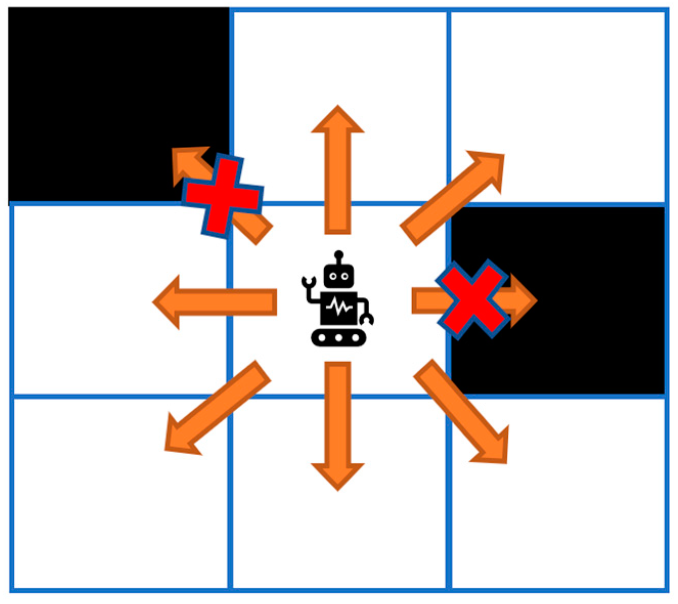
5.1. Robot Path Planning Experiment
5.2. Engineering Optimization
5.2.1. Subsubsection
5.2.2. Pressure Vessel Design
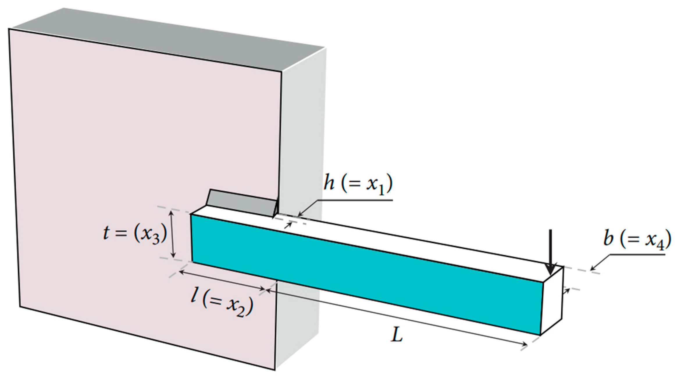
5.2.3. Tensile and Compression Spring Engineering Design
6. Conclusions
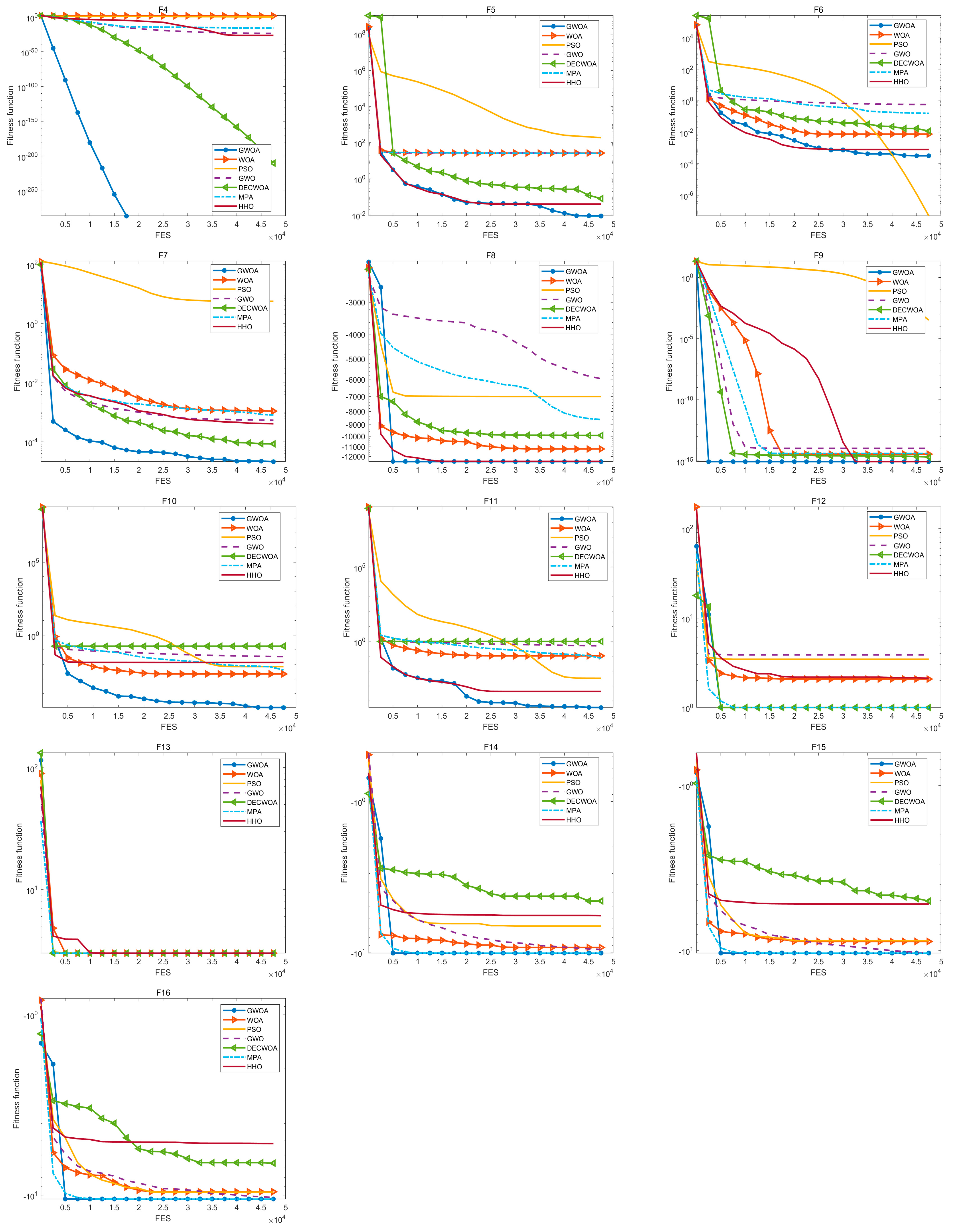
- The GWOA has better convergence accuracy and optimization results compared to the comparison algorithms, and can jump out of the local extremum when the original whale optimization algorithm falls into a local optimal function. Among the 16 functions tested in 30 dimensions, it ranked first for 12; among the 11 functions tested in 100 dimensions, it ranked first for 10.
- The GWOA has good convergence performance, incorporating nonlinear time-varying factors and inertia weights to balance the development and exploration capabilities of the WOA. To enhance the selection of the best among the population, a gravitational balance strategy was added to protect the excellent solution while increasing the trend of inferior solutions approaching the excellent solution; finally, considering the contribution of whale death to the population, a rebirth mechanism was added to help the whale algorithm jump out of local stagnation.
- The contribution experiment shows that, when the balance strategy and regeneration mechanism are added under the strategy of nonlinear time-varying factors and inertia weights, the whale optimization algorithm with balance strategy ranks first on seven functions, and the whale optimization algorithm with regeneration mechanism ranks first on eight functions. There is a performance improvement compared to the original whale algorithm; the GWOA can achieve a lead in 13 functions, but there are still shortcomings in three functions that need improvement.
- In the robot path planning experiment, the comprehensive data ranked first, and in the three classic engineering problems, the ranking was 1, 2, and 3, respectively. The overall solution accuracy was slightly different from the optimal algorithm.
- Overall, the GWOA has a good optimization performance and good robustness, and exhibits a certain uniqueness in rank sum testing. However, its optimization performance is not good enough in some functions (such as the F13 function), and its convergence speed is not fast enough in the F2, F4, F5, and F6 functions.
Author Contributions
Funding
Data Availability Statement
Conflicts of Interest
References
- Wang, R.; Feng, Y. Evaluation research on green degree of equipment manufacturing industry based on improved particle swarm optimization algorithm. Chaos Solitons Fractals Interdiscip. J. Nonlinear Sci. Nonequilibrium Complex Phenom. 2020, 131, 109502. [Google Scholar] [CrossRef]
- Abualigah, L.; Elaziz, M.A.; Khasawneh, A.M.; Alshinwan, M.; Ibrahim, R.A.; Al-Qaness, M.A.; Mirjalili, S.; Sumari, P.; Gandomi, A.H. Meta-heuristic optimization algorithms for solving real-world mechanical engineering design problems: A comprehensive survey, applications, comparative analysis, and results. Neural Comput. Appl. 2022; prepublish. [Google Scholar] [CrossRef]
- Bayzidi, H.; Talatahari, S.; Saraee, M.; Lamarche, C.P. Social Network Search for Solving Engineering Optimization Problems. Comput. Intell. Neurosci. 2021, 2021, 32. [Google Scholar] [CrossRef]
- Du, Y.; Yang, N. Analysis of image processing algorithm based on bionic intelligent optimization. Clust. Comput. 2018, 22, 3505–3512. [Google Scholar] [CrossRef]
- Chengtian, O.; Yaxian, Q.; Donglin, Z. Adaptive Spiral Flying Sparrow Search Algorithm. Sci. Program. 2021, 2021. [Google Scholar] [CrossRef]
- Rashid, A.S.; Mohamed, O.; Khalek, S.A.; Sayed, A.E.; Faihan, A.M. Optimal path planning for drones based on swarm intelligence algorithm. Neural Comput. Appl. 2022, 34, 10133–10155. [Google Scholar]
- Zhu, D.; Huang, Z.; Liao, S.; Zhou, C.; Yan, S.; Chen, G. Improved Bare Bones Particle Swarm Optimization for DNA Sequence Design. IEEE Trans. NanoBioscience 2022, 603–613. [Google Scholar] [CrossRef]
- Engy, E.-S.; Sallam, K.M.; Chakrabortty, R.K.; Abohany, A.A. A clustering based Swarm Intelligence optimization technique for the Internet of Medical Things. Expert Syst. Appl. 2021, 173, 114648. [Google Scholar]
- Mojgan, S.; FathollahiFard, A.M.; Kamyar, K.; Maziar, Y.; Mohammad, S. Selecting Appropriate Risk Response Strategies Considering Utility Function and Budget Constraints: A Case Study of a Construction Company in Iran. Buildings 2022, 12, 98. [Google Scholar]
- Eberhart, R.; Kennedy, J. A new optimizer using particle swarm theory. In Proceedings of the Mhs95 Sixth International Symposium on Micro Machine & Human Science, Nagoya, Japan, 4–6 October 1995. [Google Scholar]
- Dorigo, M. The ant system: An autocatalytic optimizing process. In Proceedings of the First European Conference on Artificial Life, Paris, France, 11–13 December 1991. [Google Scholar]
- Mirjalili, S.; Mirjalili, S.M.; Lewis, A. Grey Wolf Optimizer. Adv. Eng. Softw. 2014, 69, 46–61. [Google Scholar] [CrossRef] [Green Version]
- Fathollahi-Fard, A.M.; Hajiaghaei-Keshteli, M.; Tavakkoli-Moghaddam, R. The Social Engineering Optimizer (SEO). Eng. Appl. Artif. Intell. 2018, 72, 267–293. [Google Scholar] [CrossRef]
- Xue, J.; Shen, B. A novel swarm intelligence optimization approach: Sparrow search algorithm. Syst. Sci. Control. Eng. 2020, 8, 22–34. [Google Scholar] [CrossRef]
- Mirjalili, S.; Lewis, A. The Whale Optimization Algorithm. Adv. Eng. Softw. 2016, 95, 51–67. [Google Scholar] [CrossRef]
- Wolpert, D.H.; Macready, W.G. No free lunch theorems for optimization. IEEE Trans. Evol. Comput. 1997, 1, 67–82. [Google Scholar] [CrossRef] [Green Version]
- Xiong, G.; Zhang, J.; Shi, D.; He, Y. Parameter extraction of solar photovoltaic models using an improved whale optimization algorithm. Energy Convers. Manag. 2018, 174, 388–405. [Google Scholar] [CrossRef]
- Li, S.H.; Luo, X.H.; Wu, L.Z. An improved whale optimization algorithm for locating critical slip surface of slopes. Adv. Eng. Softw. 2021, 157, 103009. [Google Scholar] [CrossRef]
- Nadimi-Shahraki, M.H.; Zamani, H.; Mirjalili, S. Enhanced whale optimization algorithm for medical feature selection: A COVID-19 case study. Comput. Biol. Med. 2022, 148, 105858. [Google Scholar] [CrossRef]
- Yang, K.; Yang, K. Improved Whale Algorithm for Economic Load Dispatch Problem in Hydropower Plants and Comprehensive Performance Evaluation. Water Resour. Manag. 2022, 36, 5823–5838. [Google Scholar] [CrossRef]
- Shen, Y.; Zhang, C.; Gharehchopogh, F.S.; Mirjalili, S. An improved whale optimization algorithm based on multi-population evolution for global optimization and engineering design problems. Expert Syst. Appl. 2023, 215, 119269. [Google Scholar] [CrossRef]
- Guo, W.; Liu, T.; Dai, F.; Xu, P. An improved whale optimization algorithm for forecasting water resources demand. Appl. Soft Comput. 2020, 86, 105925. [Google Scholar] [CrossRef]
- Oliva, D.; Abd El Aziz, M.; Hassanien, A.E. Parameter estimation of photovoltaic cells using an improved chaotic whale optimization algorithm. Appl. Energy 2017, 200, 141–154. [Google Scholar] [CrossRef]
- Ning, G.Y.; Cao, D.Q. Improved whale optimization algorithm for solving constrained optimization problems. Discret. Dyn. Nat. Soc. 2021, 2021, 1–13. [Google Scholar] [CrossRef]
- Zhang, J.; Wang, J.S. Improved whale optimization algorithm based on nonlinear adaptive weight and golden sine operator. IEEE Access 2020, 8, 77013–77048. [Google Scholar] [CrossRef]
- Yang, W.; Xia, K.; Fan, S.; Wang, L.; Li, T.; Zhang, J.; Feng, Y. A multi-strategy Whale optimization algorithm and its application. Eng. Appl. Artif. Intell. 2022, 108, 104558. [Google Scholar] [CrossRef]
- Li, Y.; Han, M.; Guo, Q. Modified whale optimization algorithm based on tent chaotic mapping and its application in structural optimization. KSCE J. Civ. Eng. 2020, 24, 3703–3713. [Google Scholar] [CrossRef]
- Jiang, T.; Zhang, C.; Zhu, H.; Gu, J.; Deng, G. Energy-efficient scheduling for a job shop using an improved whale optimization algorithm. Mathematics 2018, 6, 220. [Google Scholar] [CrossRef] [Green Version]
- Howard, A.; Mataric, M.; Sukhatme, G.S. Mobile sensor net-work potential field: A distributed scalable solution to the area deployment using coverage problem. Distrib. Auton. Robot. Syst. 2002, 299–308. [Google Scholar] [CrossRef] [Green Version]
- Liu, L.; Zhang, R. Multistrategy Improved Whale Optimization Algorithm and Its Application. Comput. Intell. Neurosci. 2022, 2022. [Google Scholar] [CrossRef] [PubMed]
- Faramarzi, A.; Heidarinejad, M.; Mirjalili, S.; Gandomi, A.H. Marine predators algorithm:A nature-inspired metaheuristic. Expert Syst. Appl. 2020, 152, 113377. [Google Scholar] [CrossRef]
- Heidari, A.A.; Mirjalili, S.; Faris, H.; Aljarah, I.; Mafarja, M.; Chen, H. Harris hawks optimization: Algorithm and applications. Future Gener. Comput. Syst. 2019, 97, 849–872. [Google Scholar] [CrossRef]
- Ravber, M.; Liu, S.H.; Mernik, M.; Črepinšek, M. Maximum number of generations as a stopping criterion considered harmful. Appl. Soft Comput. 2022, 128, 109478. [Google Scholar] [CrossRef]
- Demšar, J. Statistical Comparisons of Classifiers over Multiple Data Sets. J. Mach. Learn. Res. 2006, 7, 1–30. [Google Scholar]
- Veček, N.; Črepinšek, M.; Mernik, M. On the influence of the number of algorithms, problems, and independent runs in the comparison of evolutionary algorithms. Appl. Soft Comput. 2017, 54, 23–45. [Google Scholar] [CrossRef]
- Akka, K.; Khaber, F. Mobile robot path planning using an improved ant colony optimization. Int. J. Adv. Robot. Syst. 2018, 15, 1729881418774673. [Google Scholar] [CrossRef] [Green Version]
- Qiuyun, T.; Hongyan, S.; Hengwei, G.; Ping, W. Improved particle swarm optimization algorithm for AGV path planning. Ieee Access 2021, 9, 33522–33531. [Google Scholar] [CrossRef]
- Zhang, H.; Zhuang, Q.; Li, G. Robot Path Planning Method Based on Indoor Spacetime Grid Model. Remote Sens. 2022, 14, 2357. [Google Scholar] [CrossRef]
- Coello, C.A.C. Use of a self-adaptive penalty approach for engineering optimization problems. Comput. Ind. 2000, 41, 113–127. [Google Scholar] [CrossRef]
- Introduction to Optimum Design; Elsevier Inc.: Amsterdam, The Netherlands, 2012.


| Function | Dim | Range | Optimum Value |
|---|---|---|---|
| 30/ 100 | [−100, 100] | 0 | |
| 30/ 100 | [−10, 10] | 0 | |
| 30/ 100 | [−100, 100] | 0 | |
| 30/ 100 | [−100, 100] | 0 | |
| 30/ 100 | [−10, 10] | 0 | |
| 30/ 100 | [−30, 30] | 0 | |
| 30/ 100 | [−1.28, 1.28] | 0 | |
| 30/ 100 | [−500, 500] | −498.5 n | |
| 30/ 100 | [−32, 32] | 0 | |
| 30/ 100 | [−50, 50] | 0 | |
| 30/ 100 | [0, ] | 0 | |
| 2 | [−65, 65] | 1 | |
| 2 | [−2, 2] | 3 | |
| 4 | [0, 10] | −10.1532 | |
| 4 | [0, 10] | −10.4028 | |
| 4 | [0, 10] | −10.5363 |
| Algorithm | Parameter Setting |
|---|---|
| WOA | |
| DECWOA | |
| GWO | |
| PSO | |
| MPA | |
| HHO | |
| GWOA |
| Function | Algorithm | Mean | Std | Best | Worst | Rank |
|---|---|---|---|---|---|---|
| F1 | DECWOA | 0.000 × 100 | 0.000 × 100 | 0.000 × 100 | 0.000 × 100 | 1 |
| GWO | 1.109 × 10−100 | 1.760 × 10−100 | 5.883 × 10−105 | 6.970 × 10−100 | 4 | |
| HHO | 4.980 × 10−55 | 1.847 × 10−54 | 2.140 × 10−66 | 9.961 × 10−54 | 5 | |
| MPA | 6.532 × 10−43 | 2.324 × 10−42 | 1.581 × 10−45 | 1.305 × 10−41 | 6 | |
| PSO | 9.451 × 10⁻¹⁰ | 1.336 × 10⁻⁹ | 4.020 × 10⁻¹¹ | 5.412 × 10⁻⁹ | 7 | |
| WOA | 1.159 × 10−201 | 0.000 × 100 | 1.382 × 10−247 | 3.478 × 10−200 | 3 | |
| GWOA | 0.000 × 100 | 0.000 × 100 | 0.000 × 100 | 0.000 × 100 | 1 | |
| F2 | DECWOA | 1.038 × 10−281 | 0.000 × 100 | 4.690 × 10−289 | 1.510 × 10−280 | 2 |
| GWO | 1.802 × 10−58 | 3.299 × 10−58 | 3.987 × 10−60 | 1.723 × 10−57 | 4 | |
| HHO | 4.471 × 10⁻²⁸ | 1.831 × 10⁻²⁷ | 5.553 × 10−36 | 1.016 × 10⁻²⁶ | 6 | |
| MPA | 1.798 × 10⁻²⁴ | 2.762 × 10⁻²⁴ | 6.237 × 10⁻²⁸ | 1.364 × 10⁻²³ | 5 | |
| PSO | 1.067 × 101 | 9.286 × 100 | 8.323 × 10⁻⁷ | 3.000 × 101 | 7 | |
| WOA | 1.766 × 10−172 | 0.000 × 100 | 1.665 × 10−187 | 5.258 × 10−171 | 3 | |
| GWOA | 0.000 × 100 | 0.000 × 100 | 0.000 × 100 | 0.000 × 100 | 1 | |
| F3 | DECWOA | 0.000 × 100 | 0.000 × 100 | 0.000 × 100 | 0.000 × 100 | 1 |
| GWO | 1.241 × 10⁻²⁶ | 4.816 × 10⁻²⁶ | 8.402 × 10⁻³⁵ | 2.395 × 10⁻²⁵ | 4 | |
| HHO | 2.361 × 10−39 | 1.040 × 10−38 | 1.402 × 10−59 | 5.788 × 10−38 | 3 | |
| MPA | 3.677 × 10⁻¹¹ | 1.532 × 10⁻¹⁰ | 5.647 × 10⁻²¹ | 8.471 × 10⁻¹⁰ | 5 | |
| PSO | 1.925 × 101 | 9.203 × 100 | 9.355 × 100 | 5.321 × 101 | 6 | |
| WOA | 8.803 × 10³ | 7.316 × 10³ | 3.430 × 10² | 2.726 × 10⁴ | 7 | |
| GWOA | 0.000 × 100 | 0.000 × 100 | 0.000 × 100 | 0.000 × 100 | 1 | |
| F4 | DECWOA | 3.418 × 10−239 | 0.000 × 100 | 8.379 × 10−252 | 7.898 × 10−238 | 2 |
| GWO | 1.583 × 10⁻²⁴ | 2.883 × 10⁻²⁴ | 1.276 × 10⁻²⁶ | 1.374 × 10⁻²³ | 4 | |
| HHO | 2.839 × 10⁻²⁷ | 1.032 × 10⁻²⁶ | 6.385 × 10⁻³⁴ | 5.218 × 10⁻²⁶ | 3 | |
| MPA | 9.160 × 10⁻¹⁷ | 7.741 × 10⁻¹⁷ | 1.150 × 10⁻¹⁷ | 3.151 × 10⁻¹⁶ | 5 | |
| PSO | 9.300 × 10⁻¹ | 2.608 × 10⁻¹ | 4.862 × 10⁻¹ | 1.577 × 100 | 6 | |
| WOA | 3.432 × 101 | 3.190 × 101 | 7.631 × 10⁻³ | 8.751 × 101 | 7 | |
| GWOA | 0.000 × 100 | 0.000 × 100 | 0.000 × 100 | 0.000 × 100 | 1 | |
| F5 | DECWOA | 7.587 × 10⁻² | 1.097 × 10⁻¹ | 2.745 × 10⁻⁵ | 4.682 × 10⁻¹ | 3 |
| GWO | 2.652 × 101 | 7.037 × 10−01 | 2.527 × 101 | 2.796 × 101 | 5 | |
| HHO | 3.959 × 10⁻² | 5.344 × 10⁻² | 2.327 × 10⁻¹ | 2.135 × 10⁻⁴ | 2 | |
| MPA | 2.558 × 101 | 6.968 × 10⁻¹ | 2.450 × 101 | 2.748 × 101 | 4 | |
| PSO | 1.785 × 10² | 5.416 × 10² | 5.711 × 100 | 3.034 × 10³ | 7 | |
| WOA | 2.655 × 101 | 6.984 × 10⁻¹ | 2.595 × 101 | 2.872 × 101 | 6 | |
| GWOA | 5.542 × 10⁻³ | 1.031 × 10⁻² | 1.539 × 10⁻⁵ | 4.511 × 10⁻² | 1 | |
| F6 | DECWOA | 1.047 × 10⁻² | 2.142 × 10⁻² | 2.228 × 10⁻⁵ | 1.200 × 10⁻¹ | 5 |
| GWO | 5.726 × 10⁻¹ | 3.101 × 10⁻¹ | 5.436 × 10⁻⁶ | 1.004 × 100 | 7 | |
| HHO | 8.034 × 10⁻⁴ | 1.490 × 10⁻³ | 6.621 × 10⁻⁸ | 6.556 × 10⁻³ | 3 | |
| MPA | 6.638 × 10⁻² | 2.771 × 10⁻² | 2.557 × 10⁻² | 1.342 × 10⁻¹ | 6 | |
| PSO | 1.174 × 10⁻⁹ | 1.511 × 10⁻⁹ | 9.635 × 10⁻¹² | 6.856 × 10⁻⁹ | 1 | |
| WOA | 7.657 × 10⁻³ | 1.318 × 10⁻² | 1.914 × 10⁻³ | 7.494 × 10⁻² | 4 | |
| GWOA | 2.213 × 10⁻⁴ | 2.728 × 10⁻⁴ | 5.203 × 10⁻⁸ | 8.539 × 10⁻⁴ | 2 | |
| F7 | DECWOA | 8.528 × 10⁻⁵ | 9.926 × 10⁻⁵ | 6.381 × 10⁻⁶ | 4.341 × 10⁻⁴ | 2 |
| GWO | 5.375 × 10⁻⁴ | 2.586 × 10⁻⁴ | 1.258 × 10⁻⁴ | 1.184 × 10⁻³ | 4 | |
| HHO | 3.872 × 10⁻⁴ | 3.588 × 10⁻⁴ | 5.965 × 10⁻⁶ | 1.845 × 10⁻³ | 3 | |
| MPA | 7.656 × 10⁻⁴ | 3.933 × 10⁻⁴ | 2.328 × 10⁻⁴ | 1.766 × 10⁻³ | 5 | |
| PSO | 5.598 × 100 | 5.362 × 100 | 2.693 × 10⁻² | 1.882 × 101 | 7 | |
| WOA | 2.162 × 10⁻³ | 1.150 × 10⁻³ | 1.952 × 10⁻⁵ | 4.614 × 10⁻³ | 6 | |
| GWOA | 2.105 × 10⁻⁵ | 1.736 × 10⁻⁵ | 6.791 × 10⁻⁷ | 6.585 × 10⁻⁵ | 1 | |
| F8 | DECWOA | −1.093 × 10⁴ | 1.556 × 10³ | −1.256 × 10⁴ | −7.419 × 10³ | 4 |
| GWO | −6.043 × 10³ | 7.729 × 10² | −7.901 × 10³ | −4.666 × 10³ | 7 | |
| HHO | −1.255 × 10⁴ | 8.996 × 101 | −1.257 × 10⁴ | −1.207 × 10⁴ | 2 | |
| MPA | −8.633 × 10³ | 5.135 × 10² | −9.670 × 10³ | −7.842 × 10³ | 5 | |
| PSO | −7.004 × 10³ | 6.751 × 10² | −8.304 × 10³ | −5.265 × 10³ | 6 | |
| WOA | −1.122 × 10⁴ | 1.609 × 10³ | −1.257 × 10⁴ | −8.155 × 10³ | 3 | |
| GWOA | −1.257 × 10⁴ | 5.298 × 10⁻³ | −1.257 × 10⁴ | −1.257 × 10⁴ | 1 | |
| F9 | DECWOA | 1.717 × 10⁻¹⁵ | 1.503 × 10⁻¹⁵ | 8.882 × 10⁻¹⁶ | 4.441 × 10⁻¹⁵ | 3 |
| GWO | 1.072 × 10⁻¹⁴ | 3.393 × 10⁻¹⁵ | 4.441 × 10⁻¹⁵ | 1.510 × 10⁻¹⁴ | 6 | |
| HHO | 8.882 × 10⁻¹⁶ | 0.000 × 100 | 8.882 × 10⁻¹⁶ | 8.882 × 10⁻¹⁶ | 2 | |
| MPA | 4.086 × 10⁻¹⁵ | 1.066 × 10⁻¹⁵ | 8.882 × 10⁻¹⁶ | 4.441 × 10⁻¹⁵ | 5 | |
| PSO | 4.697 × 10−05 | 5.923 × 10−05 | 3.723 × 10−06 | 2.387 × 10−04 | 7 | |
| WOA | 3.612 × 10⁻¹⁵ | 2.371 × 10⁻¹⁵ | 8.882 × 10⁻¹⁶ | 7.994 × 10⁻¹⁵ | 4 | |
| GWOA | 8.882 × 10⁻¹⁶ | 0.000 × 100 | 8.882 × 10⁻¹⁶ | 8.882 × 10⁻¹⁶ | 1 | |
| F10 | DECWOA | 1.761 × 10⁻¹ | 1.223 × 10⁻¹ | 4.751 × 10⁻² | 4.687 × 10⁻¹ | 7 |
| GWO | 3.382 × 10⁻² | 1.810 × 10⁻² | 6.540 × 10⁻³ | 7.931 × 10⁻² | 6 | |
| HHO | 1.337 × 10⁻² | 1.514 × 10⁻² | 3.056 × 10⁻⁶ | 6.628 × 10⁻² | 5 | |
| MPA | 1.654 × 10⁻³ | 1.139 × 10⁻³ | 3.977 × 10⁻⁴ | 5.364 × 10⁻³ | 2 | |
| PSO | 6.911 × 10⁻³ | 2.586 × 10⁻² | 1.771 × 10⁻¹³ | 1.037 × 10−01 | 4 | |
| WOA | 2.197 × 10⁻³ | 3.159 × 10⁻³ | 2.711 × 10⁻⁴ | 1.392 × 10⁻² | 3 | |
| GWOA | 6.194 × 10⁻⁶ | 1.370 × 10⁻⁵ | 6.630 × 10⁻¹⁰ | 7.023 × 10⁻⁵ | 1 | |
| F11 | DECWOA | 9.795 × 10⁻¹ | 2.554 × 10⁻¹ | 2.336 × 10⁻¹ | 1.450 × 100 | 7 |
| GWO | 4.945 × 10⁻¹ | 2.342 × 10⁻¹ | 9.743 × 10⁻² | 1.120 × 100 | 6 | |
| HHO | 4.249 × 10⁻⁴ | 5.236 × 10⁻⁴ | 5.594 × 10⁻¹¹ | 1.954 × 10⁻³ | 2 | |
| MPA | 3.575 × 10⁻² | 2.176 × 10⁻² | 5.093 × 10⁻³ | 9.639 × 10⁻² | 4 | |
| PSO | 3.296 × 10⁻³ | 5.035 × 10⁻³ | 1.775 × 10⁻¹¹ | 1.099 × 10⁻² | 3 | |
| WOA | 1.061 × 10⁻¹ | 1.075 × 10⁻¹ | 8.354 × 10⁻³ | 3.793 × 10⁻¹ | 5 | |
| GWOA | 6.110 × 10⁻⁵ | 4.245 × 10⁻⁵ | 3.741 × 10⁻⁸ | 2.120 × 10⁻⁴ | 1 | |
| F12 | DECWOA | 9.980 × 10⁻¹ | 0.000 × 100 | 9.980 × 10⁻¹ | 9.980 × 10⁻¹ | 1 |
| GWO | 3.874 × 100 | 3.724 × 100 | 9.980 × 10⁻¹ | 1.267 × 101 | 7 | |
| HHO | 2.119 × 100 | 1.646 × 100 | 9.980 × 10⁻¹ | 5.929 × 100 | 5 | |
| MPA | 9.980 × 10⁻¹ | 0.000 × 100 | 9.980 × 10⁻¹ | 9.980 × 10⁻¹ | 1 | |
| PSO | 3.463 × 100 | 2.478 × 100 | 9.980 × 10⁻¹ | 1.076 × 101 | 6 | |
| WOA | 2.079 × 100 | 2.451 × 100 | 9.980 × 10⁻¹ | 1.076 × 101 | 4 | |
| GWOA | 9.980 × 10⁻¹ | 0.000 × 100 | 9.980 × 10⁻¹ | 9.980 × 10⁻¹ | 1 | |
| F13 | DECWOA | 3.000 × 100 | 2.153 × 10⁻⁴ | 3.000 × 100 | 3.001 × 100 | 6 |
| GWO | 3.000 × 100 | 3.260 × 10⁻⁶ | 3.000 × 100 | 3.000 × 100 | 3 | |
| HHO | 3.000 × 100 | 1.271 × 10⁻⁵ | 3.000 × 100 | 3.000 × 100 | 4 | |
| MPA | 3.000 × 100 | 1.240 × 10⁻¹⁵ | 3.000 × 100 | 3.000 × 100 | 1 | |
| PSO | 3.000 × 100 | 1.347 × 10⁻¹⁵ | 3.000 × 100 | 3.000 × 100 | 5 | |
| WOA | 3.000 × 100 | 1.236 × 10⁻⁵ | 3.000 × 100 | 3.000 × 100 | 4 | |
| GWOA | 3.000 × 100 | 3.507 × 10⁻³ | 3.000 × 100 | 3.015 × 100 | 7 | |
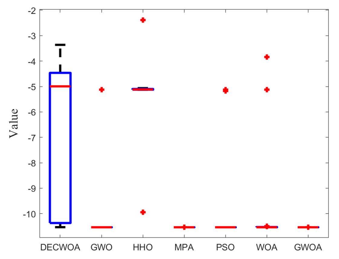
| F14 | DECWOA | −5.146 × 100 | 2.326 × 100 | −9.879 × 100 | −2.435 × 100 | 7 |
| GWO | −9.646 × 100 | 1.520 × 100 | −1.015 × 101 | −5.055 × 100 | 3 | |
| HHO | −5.739 × 100 | 1.614 × 100 | −1.011 × 101 | −4.924 × 100 | 6 | |
| MPA | −1.015 × 101 | 5.299 × 10⁻¹⁵ | −1.015 × 101 | −1.015 × 101 | 1 | |
| PSO | −6.708 × 100 | 2.936 × 100 | −1.015 × 101 | −2.630 × 100 | 5 | |
| WOA | −9.303 × 100 | 1.900 × 100 | −1.015 × 101 | −5.055 × 100 | 4 | |
| GWOA | −1.015 × 101 | 6.019 × 10−05 | −1.015 × 101 | −1.015 × 101 | 2 | |
| F15 | DECWOA | −5.217 × 100 | 2.150 × 100 | −1.002 × 101 | −2.325 × 100 | 7 |
| GWO | −1.040 × 101 | 9.969 × 10⁻⁵ | −1.040 × 101 | −1.040 × 101 | 3 | |
| HHO | −5.237 × 100 | 9.564 × 10⁻¹ | −1.038 × 101 | −4.937 × 100 | 6 | |
| MPA | −1.040 × 101 | 1.376 × 10⁻¹⁵ | −1.040 × 101 | −1.040 × 101 | 1 | |
| PSO | −8.738 × 100 | 2.575 × 100 | −1.040 × 101 | −2.766 × 100 | 5 | |
| WOA | −8.830 × 100 | 2.658 × 100 | −1.040 × 101 | −2.766 × 100 | 4 | |
| GWOA | −1.040 × 101 | 5.405 × 10⁻⁵ | −1.040 × 101 | −1.040 × 101 | 2 | |
| F16 | DECWOA | −6.657 × 100 | 2.796 × 100 | −1.053 × 101 | −3.362 × 100 | 6 |
| GWO | −1.036 × 101 | 9.707 × 10⁻¹ | −1.054 × 101 | −5.128 × 100 | 3 | |
| HHO | −5.180 × 100 | 1.011 × 100 | −9.945 × 100 | −2.382 × 100 | 7 | |
| MPA | −1.054 × 101 | 1.020 × 10⁻¹⁴ | −1.054 × 101 | −1.054 × 101 | 1 | |
| PSO | −9.637 × 100 | 2.012 × 100 | −5.128 × 100 | −1.054 × 101 | 4 | |
| WOA | −9.589 × 100 | 2.121 × 100 | −1.054 × 101 | −3.835 × 100 | 5 | |
| GWOA | −1.054 × 101 | 8.819 × 10⁻⁵ | −1.054 × 101 | −1.054 × 101 | 2 |
| Function | Algorithm | Mean | Std | Best | Worst | Rank |
|---|---|---|---|---|---|---|
| F1 | DECWOA | 0.000 × 100 | 0.000 × 100 | 0.000 × 100 | 0.000 × 100 | 1 |
| GWO | 4.767 × 10−52 | 6.152 × 10−52 | 1.652 × 10−53 | 2.762 × 10−51 | 4 | |
| HHO | 4.289 × 10−51 | 2.253 × 10−50 | 1.536 × 10−63 | 1.256 × 10−49 | 5 | |
| MPA | 7.552 × 10−37 | 2.216 × 10−36 | 1.013 × 10−39 | 1.063 × 10⁻³⁵ | 6 | |
| PSO | 4.476 × 100 | 2.353 × 100 | 1.966 × 100 | 1.466 × 101 | 7 | |
| WOA | 8.745 × 10−249 | 0.000 × 100 | 3.406 × 10−281 | 2.367 × 10−247 | 3 | |
| GWOA | 0.000 × 100 | 0.000 × 100 | 0.000 × 100 | 0.000 × 100 | 1 | |
| F2 | DECWOA | 2.121 × 10−280 | 0.000 × 100 | 1.711 × 10−288 | 5.598 × 10−279 | 2 |
| GWO | 3.760 × 10⁻³¹ | 2.429 × 10⁻³¹ | 6.812 × 10⁻³² | 9.339 × 10⁻³¹ | 4 | |
| HHO | 5.974 × 10⁻²⁷ | 2.200 × 10⁻²⁶ | 1.261 × 10⁻³² | 9.778 × 10⁻²⁶ | 5 | |
| MPA | 1.433 × 10⁻²¹ | 2.219 × 10⁻²¹ | 9.374 × 10⁻²³ | 1.165 × 10⁻²⁰ | 6 | |
| PSO | 1.330 × 10² | 3.058 × 101 | 7.062 × 101 | 2.022 × 10² | 7 | |
| WOA | 6.285 × 10−173 | 0.000 × 100 | 7.623 × 10−186 | 9.895 × 10−172 | 3 | |
| GWOA | 0.000 × 100 | 0.000 × 100 | 0.000 × 100 | 0.000 × 100 | 1 | |
| F3 | DECWOA | 3.284 × 10−300 | 0.000 × 100 | 0.000 × 100 | 9.850 × 10−299 | 2 |
| GWO | 8.879 × 10⁻² | 2.704 × 10⁻¹ | 5.568 × 10⁻⁸ | 1.099 × 100 | 5 | |
| HHO | 2.418 × 10⁻²² | 6.512 × 10⁻²² | 5.585 × 10−59 | 3.628 × 10⁻²¹ | 3 | |
| MPA | 3.422 × 10⁻³ | 4.402 × 10⁻³ | 3.841 × 10⁻⁸ | 1.647 × 10⁻² | 4 | |
| PSO | 1.402 × 10⁴ | 3.849 × 10³ | 8.340 × 10³ | 3.029 × 10⁴ | 6 | |
| WOA | 6.921 × 10⁵ | 1.518 × 10⁵ | 3.080 × 10⁵ | 1.010 × 10⁶ | 7 | |
| GWOA | 0.000 × 100 | 0.000 × 100 | 0.000 × 100 | 0.000 × 100 | 1 | |
| F4 | DECWOA | 4.888 × 10−238 | 0.000 × 100 | 2.822 × 10−250 | 1.264 × 10−236 | 2 |
| GWO | 1.798 × 10⁻⁶ | 4.767 × 10⁻⁶ | 5.242 × 10⁻¹⁰ | 1.988 × 10⁻⁵ | 5 | |
| HHO | 1.672 × 10⁻²⁶ | 1.034 × 10⁻²⁵ | 6.348 × 10⁻³³ | 4.837 × 10⁻²⁵ | 3 | |
| MPA | 6.422 × 10⁻¹⁴ | 4.993 × 10⁻¹⁴ | 1.003 × 10⁻¹⁴ | 2.731 × 10⁻¹³ | 4 | |
| PSO | 1.047 × 101 | 1.067 × 100 | 7.704 × 100 | 2.631 × 101 | 6 | |
| WOA | 7.355 × 101 | 2.539 × 101 | 1.574 × 101 | 9.677 × 101 | 7 | |
| GWOA | 0.000 × 100 | 0.000 × 100 | 0.000 × 100 | 0.000 × 100 | 1 | |
| F5 | DECWOA | 7.731 × 10⁻² | 1.680 × 10⁻¹ | 9.121 × 10⁻⁶ | 8.441 × 10⁻¹ | 2 |
| GWO | 9.757 × 101 | 7.703 × 10⁻¹ | 9.608 × 101 | 9.844 × 101 | 5 | |
| HHO | 1.032 × 10⁻¹ | 1.659 × 10⁻¹ | 3.784 × 10⁻⁶ | 8.328 × 10⁻¹ | 3 | |
| MPA | 9.762 × 101 | 6.992 × 10⁻¹ | 9.609 × 101 | 9.848 × 101 | 6 | |
| PSO | 1.089 × 10⁴ | 1.644 × 10⁴ | 2.919 × 10³ | 9.666 × 10⁴ | 7 | |
| WOA | 9.713 × 101 | 5.503 × 10⁻¹ | 9.641 × 101 | 9.818 × 101 | 4 | |
| GWOA | 6.354 × 10⁻³ | 8.316 × 10⁻³ | 8.213 × 10⁻⁵ | 3.236 × 10⁻² | 1 | |
| F6 | DECWOA | 7.564 × 100 | 2.046 × 100 | 2.046 × 100 | 1.548 × 101 | 4 |
| GWO | 9.311 × 100 | 9.871 × 10⁻¹ | 7.506 × 100 | 1.151 × 101 | 6 | |
| HHO | 1.600 × 10⁻³ | 1.563 × 10⁻³ | 2.680 × 10⁻⁶ | 5.413 × 10⁻³ | 2 | |
| MPA | 8.759 × 100 | 1.125 × 100 | 6.888 × 100 | 1.110 × 101 | 5 | |
| PSO | 1.271 × 101 | 4.203 × 100 | 1.641 × 100 | 1.835 × 101 | 7 | |
| WOA | 6.353 × 10⁻¹ | 2.295 × 10⁻¹ | 2.935 × 10⁻¹ | 1.179 × 100 | 3 | |
| GWOA | 6.107 × 10⁻⁴ | 7.569 × 10⁻⁴ | 2.193 × 10⁻³ | 9.506 × 10⁻⁷ | 1 | |
| F7 | DECWOA | 1.074 × 10⁻⁴ | 1.202 × 10⁻⁴ | 3.821 × 10⁻⁶ | 5.318 × 10⁻⁴ | 2 |
| GWO | 1.367 × 10⁻³ | 6.785 × 10⁻⁴ | 4.672 × 10⁻⁴ | 3.082 × 10⁻³ | 6 | |
| HHO | 3.580 × 10⁻⁴ | 3.410 × 10⁻⁴ | 1.990 × 10⁻⁵ | 1.467 × 10⁻³ | 3 | |
| MPA | 1.241 × 10⁻³ | 5.527 × 10⁻⁴ | 3.081 × 10⁻⁴ | 2.415 × 10⁻³ | 5 | |
| PSO | 2.465 × 10² | 1.131 × 10² | 5.989 × 101 | 6.061 × 10² | 7 | |
| WOA | 1.162 × 10⁻³ | 1.860 × 10⁻³ | 8.025 × 10⁻⁵ | 9.878 × 10⁻³ | 4 | |
| GWOA | 8.503 × 10⁻⁵ | 5.969 × 10⁻⁵ | 2.406 × 10⁻⁶ | 3.279 × 10⁻⁴ | 1 | |
| F8 | DECWOA | −3.594 × 10⁴ | 7.935 × 10³ | −4.190 × 10⁴ | −1.530 × 10⁴ | 3 |
| GWO | −1.674 × 10⁴ | 2.410 × 10³ | −2.007 × 10⁴ | −6.180 × 10³ | 7 | |
| HHO | −4.151 × 10⁴ | 1.693 × 10³ | −4.190 × 10⁴ | −3.254 × 10⁴ | 2 | |
| MPA | −2.054 × 10⁴ | 1.297 × 10³ | −2.354 × 10⁴ | −1.800 × 10⁴ | 6 | |
| PSO | −2.122 × 10⁴ | 1.871 × 10³ | −2.488 × 10⁴ | −1.633 × 10⁴ | 5 | |
| WOA | −3.504 × 10⁴ | 6.199 × 10³ | −4.190 × 10⁴ | −2.708 × 10⁴ | 4 | |
| GWOA | −4.190 × 10⁴ | 2.467 × 10⁻² | −4.190 × 10⁴ | −4.190 × 10⁴ | 1 | |
| F9 | DECWOA | 1.480 × 10⁻¹⁵ | 1.324 × 10⁻¹⁵ | 4.441 × 10⁻¹⁵ | 8.882 × 10⁻¹⁶ | 3 |
| GWO | 3.393 × 10⁻¹⁴ | 4.118 × 10⁻¹⁵ | 2.576 × 10⁻¹⁴ | 3.997 × 10⁻¹⁴ | 6 | |
| HHO | 8.882 × 10⁻¹⁶ | 0.000 × 100 | 8.882 × 10⁻¹⁶ | 8.882 × 10⁻¹⁶ | 1 | |
| MPA | 4.441 × 10⁻¹⁵ | 0.000 × 100 | 4.441 × 10⁻¹⁵ | 4.441 × 10⁻¹⁵ | 5 | |
| PSO | 3.117 × 100 | 1.421 × 100 | 2.134 × 100 | 1.054 × 101 | 7 | |
| WOA | 3.730 × 10⁻¹⁵ | 2.321 × 10⁻¹⁵ | 8.882 × 10⁻¹⁶ | 7.994 × 10⁻¹⁵ | 4 | |
| GWOA | 8.882 × 10⁻¹⁶ | 0.000 × 100 | 8.882 × 10⁻¹⁶ | 8.882 × 10⁻¹⁶ | 1 | |
| F10 | DECWOA | 1.361 × 10⁻¹ | 4.666 × 10⁻² | 7.870 × 10⁻² | 2.776 × 10⁻¹ | 5 |
| GWO | 2.441 × 10⁻¹ | 6.136 × 10⁻² | 1.489 × 10⁻¹ | 4.127 × 10⁻¹ | 6 | |
| HHO | 1.065 × 10⁻⁵ | 1.547 × 10⁻⁵ | 3.754 × 10⁻⁸ | 6.632 × 10⁻⁵ | 2 | |
| MPA | 1.256 × 10⁻¹ | 3.040 × 10⁻² | 8.727 × 10⁻² | 2.134 × 10⁻¹ | 4 | |
| PSO | 2.223 × 100 | 8.594 × 10⁻¹ | 8.134 × 10⁻¹ | 4.035 × 100 | 7 | |
| WOA | 7.379 × 10⁻³ | 1.122 × 10⁻² | 2.556 × 10⁻³ | 6.692 × 10⁻² | 3 | |
| GWOA | 2.117 × 10⁻⁶ | 2.512 × 10⁻⁶ | 4.615 × 10⁻⁹ | 1.084 × 10⁻⁵ | 1 | |
| F11 | DECWOA | 3.791 × 100 | 1.362 × 100 | 1.841 × 100 | 7.195 × 100 | 4 |
| GWO | 6.154 × 100 | 3.653 × 10⁻¹ | 5.562 × 100 | 6.847 × 100 | 5 | |
| HHO | 2.725 × 10⁻⁴ | 2.417 × 10⁻⁴ | 4.121 × 10⁻⁷ | 9.645 × 10⁻⁴ | 2 | |
| MPA | 8.861 × 100 | 1.438 × 100 | 4.728 × 100 | 9.704 × 100 | 6 | |
| PSO | 5.850 × 101 | 1.642 × 101 | 2.893 × 101 | 8.736 × 101 | 7 | |
| WOA | 1.016 × 100 | 4.636 × 10⁻¹ | 3.253 × 10⁻¹ | 2.274 × 100 | 3 | |
| GWOA | 5.125 × 10⁻⁵ | 7.072 × 10⁻⁵ | 3.475 × 10⁻⁹ | 2.589 × 10⁻⁴ | 1 |
| Function | Index | WOA | WOA-1 | WOA-2 | WOA-3 | WOA-4 | GWOA |
|---|---|---|---|---|---|---|---|
| F1 | Mean | 3.046 × 10−71 | 1.797 × 10−104 | 8.514 × 10−248 | 0.000 × 100 | 0.000 × 100 | 0.000 × 100 |
| Std | 1.639 × 10−70 | 6.244 × 10−104 | 0.000 × 100 | 0.000 × 100 | 0.000 × 100 | 0.000 × 100 | |
| Best | 5.624 × 10−86 | 5.817 × 10−115 | 1.234 × 10−274 | 0.000 × 100 | 0.000 × 100 | 0.000 × 100 | |
| Worst | 9.135 × 10−70 | 2.846 × 10−103 | 1.252 × 10−246 | 0.000 × 100 | 0.000 × 100 | 0.000 × 100 | |
| F2 | Mean | 1.810 × 10−51 | 2.917 × 10−67 | 6.176 × 10−136 | 0.000 × 100 | 5.771 × 10−223 | 2.616 × 10−227 |
| Std | 4.928 × 10−51 | 1.224 × 10−66 | 1.830 × 10−135 | 0.000 × 100 | 0.000 × 100 | 0.000 × 100 | |
| Best | 3.145 × 10−57 | 7.767 × 10−75 | 5.150 × 10−150 | 0.000 × 100 | 5.765 × 10−255 | 1.203 × 10−270 | |
| Worst | 2.668 × 10−50 | 5.625 × 10−66 | 8.052 × 10−135 | 0.000 × 100 | 1.076 × 10−221 | 7.847 × 10−226 | |
| F3 | Mean | 4.390 × 10⁴ | 2.893 × 10⁴ | 7.764 × 10−179 | 0.000 × 100 | 0.000 × 100 | 0.000 × 100 |
| Std | 1.312 × 10⁴ | 1.488 × 10⁴ | 0.000 × 100 | 0.000 × 100 | 0.000 × 100 | 0.000 × 100 | |
| Best | 1.659 × 10⁴ | 1.385 × 10³ | 3.409 × 10−217 | 0.000 × 100 | 0.000 × 100 | 0.000 × 100 | |
| Worst | 7.255 × 10⁴ | 5.585 × 10⁴ | 1.553 × 10−177 | 0.000 × 100 | 0.000 × 100 | 0.000 × 100 | |
| F4 | Mean | 4.861 × 101 | 8.027 × 101 | 3.220 × 10−108 | 0.000 × 100 | 5.683 × 10−230 | 1.586 × 10−233 |
| Std | 2.601 × 101 | 1.516 × 101 | 1.403 × 10−107 | 0.000 × 100 | 0.000 × 100 | 0.000 × 100 | |
| Best | 5.627 × 100 | 3.321 × 101 | 4.010 × 10−120 | 0.000 × 100 | 1.100 × 10−246 | 4.056 × 10−277 | |
| Worst | 8.861 × 101 | 9.271 × 101 | 6.438 × 10−107 | 0.000 × 100 | 1.108 × 10−228 | 4.130 × 10−232 | |
| F5 | Mean | 2.803 × 101 | 2.879 × 101 | 2.877 × 101 | 2.877 × 101 | 4.630 × 10⁻² | 5.944 × 10⁻³ |
| Std | 3.640 × 10⁻¹ | 2.571 × 10⁻² | 2.166 × 10⁻² | 2.244 × 10⁻² | 6.285 × 10⁻² | 6.671 × 10⁻³ | |
| Best | 2.749 × 101 | 2.874 × 101 | 2.873 × 101 | 2.871 × 101 | 7.328 × 10⁻⁶ | 2.331 × 10⁻⁷ | |
| Worst | 2.876 × 101 | 2.885 × 101 | 2.880 × 101 | 2.882 × 101 | 2.307 × 10⁻¹ | 2.815 × 10⁻² | |
| F6 | Mean | 3.828 × 10⁻¹ | 2.477 × 100 | 7.878 × 10⁻¹ | 6.386 × 10⁻¹ | 4.702 × 10⁻³ | 2.553 × 10⁻³ |
| Std | 2.616 × 10⁻¹ | 3.087 × 10⁻¹ | 3.985 × 10⁻¹ | 2.817 × 10⁻¹ | 2.611 × 10⁻³ | 3.258 × 10⁻³ | |
| Best | 8.880 × 10⁻² | 1.941 × 100 | 1.840 × 10⁻¹ | 7.272 × 10⁻² | 1.170 × 10⁻⁴ | 9.584 × 10⁻⁶ | |
| Worst | 1.169 × 100 | 2.965 × 100 | 1.765 × 100 | 9.993 × 10⁻¹ | 7.972 × 10⁻³ | 1.484 × 10⁻² | |
| F7 | Mean | 4.958 × 10⁻³ | 2.235 × 10⁻³ | 7.719 × 10⁻⁵ | 6.720 × 10⁻⁵ | 3.636 × 10⁻⁴ | 2.713 × 10⁻⁵ |
| Std | 6.545 × 10⁻³ | 1.988 × 10⁻³ | 5.770 × 10⁻⁵ | 5.441 × 10⁻⁵ | 3.005 × 10⁻⁴ | 2.563 × 10⁻⁵ | |
| Best | 4.967 × 10⁻⁵ | 1.018 × 10⁻⁴ | 8.626 × 10⁻⁶ | 7.830 × 10⁻⁸ | 3.213 × 10⁻⁵ | 1.628 × 10⁻⁶ | |
| Worst | 3.094 × 10⁻² | 6.387 × 10⁻³ | 1.787 × 10⁻⁴ | 1.910 × 10⁻⁴ | 9.762 × 10⁻⁴ | 8.928 × 10⁻⁵ | |
| F8 | Mean | −1.044 × 10⁴ | −6.838 × 10³ | −1.183 × 10⁴ | −1.257 × 10⁴ | −1.257 × 10⁴ | −1.257 × 10⁴ |
| Std | 1.745 × 10³ | 1.988 × 10² | 7.802 × 10² | 1.192 × 10⁻¹ | 9.278 × 10⁻² | 1.932 × 10⁻¹ | |
| Best | −1.257 × 10⁴ | −1.184 × 10⁴ | −1.257 × 10⁴ | −1.257 × 10⁴ | −1.257 × 10⁴ | −1.257 × 10⁴ | |
| Worst | −6.624 × 10³ | −3.409 × 10³ | −1.033 × 10⁴ | −1.257 × 10⁴ | −1.257 × 10⁴ | −1.257 × 10⁴ | |
| F9 | Mean | 2.901 × 10⁻¹⁵ | 3.908 × 10⁻¹⁵ | 8.882 × 10⁻¹⁶ | 8.882 × 10⁻¹⁶ | 8.882 × 10⁻¹⁶ | 8.882 × 10⁻¹⁶ |
| Std | 2.543 × 10⁻¹⁵ | 2.814 × 10⁻¹⁵ | 0.000 × 100 | 0.000 × 100 | 0.000 × 100 | 0.000 × 100 | |
| Best | 8.882 × 10⁻¹⁶ | 8.882 × 10⁻¹⁶ | 8.882 × 10⁻¹⁶ | 8.882 × 10⁻¹⁶ | 8.882 × 10⁻¹⁶ | 8.882 × 10⁻¹⁶ | |
| Worst | 7.994 × 10⁻¹⁵ | 7.994 × 10⁻¹⁵ | 8.882 × 10⁻¹⁶ | 8.882 × 10⁻¹⁶ | 8.882 × 10⁻¹⁶ | 8.882 × 10⁻¹⁶ | |
| F10 | Mean | 2.246 × 10⁻² | 3.384 × 10⁻¹ | 1.155 × 10⁻¹ | 3.522 × 10⁻² | 3.009 × 10⁻⁵ | 4.793 × 10⁻⁶ |
| Std | 1.458 × 10⁻² | 2.090 × 10⁻¹ | 8.382 × 10⁻² | 2.210 × 10⁻² | 2.730 × 10⁻⁵ | 6.325 × 10⁻⁶ | |
| Best | 5.130 × 10⁻³ | 9.040 × 10⁻² | 1.430 × 10⁻² | 1.202 × 10⁻² | 9.999 × 10⁻⁷ | 7.593 × 10⁻⁸ | |
| Worst | 5.779 × 10⁻² | 6.623 × 10⁻¹ | 3.012 × 10⁻¹ | 8.957 × 10⁻² | 9.420 × 10⁻⁵ | 2.805 × 10⁻⁵ | |
| F11 | Mean | 6.729 × 10⁻¹ | 1.581 × 100 | 5.807 × 10⁻¹ | 4.446 × 10⁻¹ | 2.019 × 10⁻⁴ | 8.990 × 10⁻⁵ |
| Std | 2.858 × 10⁻¹ | 5.461 × 10⁻¹ | 3.515 × 10⁻¹ | 2.270 × 10⁻¹ | 2.366 × 10⁻⁴ | 1.910 × 10⁻⁴ | |
| Best | 1.035 × 10⁻¹ | 6.989 × 10⁻¹ | 9.693 × 10⁻² | 7.115 × 10⁻² | 1.752 × 10⁻⁶ | 1.175 × 10⁻⁷ | |
| Worst | 1.254 × 100 | 2.590 × 100 | 1.336 × 100 | 9.332 × 10⁻¹ | 7.285 × 10⁻⁴ | 9.061 × 10⁻⁴ | |
| F12 | Mean | 2.278 × 100 | 7.246 × 100 | 2.256 × 100 | 2.977 × 100 | 9.980 × 10⁻¹ | 9.980 × 10⁻¹ |
| Std | 2.448 × 100 | 4.901 × 100 | 7.676 × 10⁻¹ | 4.936 × 10⁻¹ | 0.000 × 100 | 0.000 × 100 | |
| Best | 9.980 × 10⁻¹ | 9.983 × 10⁻¹ | 9.980 × 10⁻¹ | 9.980 × 10⁻¹ | 9.980 × 10⁻¹ | 9.980 × 10⁻¹ | |
| Worst | 1.076 × 101 | 1.550 × 101 | 3.093 × 100 | 3.835 × 100 | 9.980 × 10⁻¹ | 9.980 × 10⁻¹ | |
| F13 | Mean | 3.000 × 100 | 3.000 × 100 | 3.000 × 100 | 3.000 × 100 | 3.569 × 100 | 3.014 × 100 |
| Std | 8.684 × 10⁻⁵ | 8.360 × 10⁻³ | 1.175 × 10⁻³ | 1.326 × 10⁻⁴ | 7.881 × 10⁻¹ | 5.108 × 10⁻² | |
| Best | 3.000 × 100 | 3.000 × 100 | 3.000 × 100 | 3.000 × 100 | 3.000 × 100 | 3.000 × 100 | |
| Worst | 3.000 × 100 | 3.038 × 100 | 3.004 × 100 | 3.000 × 100 | 5.842 × 100 | 3.275 × 100 | |
| F14 | Mean | −8.278 × 100 | −7.556 × 100 | −9.327 × 100 | −9.599 × 100 | −1.015 × 101 | −1.015 × 101 |
| Std | 2.681 × 100 | 1.364 × 100 | 9.704 × 10⁻¹ | 6.138 × 10⁻¹ | 1.130 × 10⁻⁵ | 5.371 × 10⁻⁵ | |
| Best | −1.015 × 101 | −1.040 × 101 | −1.040 × 101 | −1.015 × 101 | −1.015 × 101 | −1.015 × 101 | |
| Worst | −2.627 × 100 | −4.287 × 100 | −6.550 × 100 | −8.635 × 100 | −1.015 × 101 | −1.015 × 101 | |
| F15 | Mean | −7.213 × 100 | −6.511 × 101 | −9.591 × 101 | −9.885 × 100 | −1.040 × 101 | −1.040 × 101 |
| Std | 3.015 × 100 | 1.996 × 100 | 1.091 × 100 | 2.506 × 100 | 1.078 × 10⁻⁵ | 8.550 × 10⁻⁵ | |
| Best | −1.040 × 101 | −1.040 × 101 | −1.040 × 101 | −1.974 × 101 | −1.040 × 101 | −1.040 × 101 | |
| Worst | −2.766 × 100 | −4.187 × 100 | −7.032 × 100 | −5.053 × 100 | −1.040 × 101 | −1.040 × 101 | |
| F16 | Mean | −7.214 × 100 | −7.377 × 100 | −10.09 × 101 | −9.949 × 100 | −1.054 × 101 | −1.054 × 101 |
| Std | 3.206 × 100 | 2.069 × 100 | 7.744 × 100 | 7.981 × 10⁻¹ | 9.72 × 10⁻⁵ | 9.409 × 10⁻⁵ | |
| Best | −1.054 × 101 | −1.054 × 101 | −1.054 × 101 | −1.054 × 101 | −1.054 × 101 | −1.054 × 101 | |
| Worst | −1.859 × 100 | −3.405 × 100 | −7.107 × 100 | −8.468 × 100 | −1.054 × 101 | −1.054 × 101 | |
| Optimal number of indicators | 1 | 1 | 2 | 7 | 8 | 13 | |
| Algorithm | DECWOA | WOA | GWO | PSO | HHO | MPA |
|---|---|---|---|---|---|---|
| F1 | 1.21 × 10⁻¹² | 1.21 × 10⁻¹² | 1.21 × 10⁻¹² | 1.21 × 10⁻¹² | 1.21 × 10⁻¹² | 1.21 × 10⁻¹² |
| F2 | 3.01 × 10⁻¹¹ | 3.01 × 10⁻¹¹ | 3.01 × 10⁻¹¹ | 3.01 × 10⁻¹¹ | 3.01 × 10⁻¹¹ | 3.01 × 10⁻¹¹ |
| F3 | 4.56 × 10⁻¹¹ | 1.21 × 10⁻¹² | 1.21 × 10⁻¹² | 2.36 × 10⁻¹² | 1.21 × 10⁻¹² | 1.21 × 10⁻¹² |
| F4 | 3.01 × 10⁻¹¹ | 3.01 × 10⁻¹¹ | 3.01 × 10⁻¹¹ | 3.01 × 10⁻¹¹ | 3.01 × 10⁻¹¹ | 3.01 × 10⁻¹¹ |
| F5 | 3.01 × 10⁻¹¹ | 3.01 × 10⁻¹¹ | 3.01 × 10⁻¹¹ | 3.01 × 10⁻¹¹ | 6.76 × 10⁻⁵ | 3.01 × 10⁻¹¹ |
| F6 | 3.01 × 10⁻¹¹ | 3.01 × 10⁻¹¹ | 5.07 × 10⁻¹⁰ | 2.31 × 10⁻⁶ | 2.83 × 10⁻⁴ | 3.15 × 10⁻¹⁰ |
| F7 | 2.12 × 10⁻⁴ | 1.15 × 10⁻⁷ | 7.77 × 10⁻⁹ | 3.01 × 10⁻¹¹ | 2.68 × 10⁻⁴ | 5.53 × 10⁻⁸ |
| F8 | 2.12 × 10⁻⁴ | 3.68 × 10⁻¹¹ | 3.01 × 10⁻¹¹ | 3.01 × 10⁻¹¹ | 5.57 × 10⁻¹⁰ | 3.01 × 10⁻¹¹ |
| F9 | 4.29 × 10⁻¹⁰ | 7.46 × 10⁻⁷ | 1.10 × 10⁻¹² | 1.21 × 10⁻¹² | 5.34 × 10⁻⁶ | 1.19 × 10⁻¹² |
| F10 | 2.12 × 10⁻⁴ | 3.01 × 10⁻¹¹ | 3.01 × 10⁻¹¹ | 2.38 × 10⁻⁸ | 6.51 × 10⁻⁹ | 3.01 × 10⁻¹¹ |
| F11 | 3.01 × 10⁻¹¹ | 3.01 × 10⁻¹¹ | 2.15 × 10⁻⁶ | 1.59 × 10⁻³ | 2.19 × 10⁻⁷ | 3.68 × 10⁻¹¹ |
| F12 | 3.01 × 10⁻¹¹ | 1.10 × 10⁻³ | 9.03 × 10⁻⁴ | 6.67 × 10⁻⁵ | 2.19 × 10⁻⁷ | 1.36 × 10⁻¹¹ |
| F13 | 9.21 × 10⁻⁵ | 4.80 × 10⁻⁷ | 6.73 × 10⁻⁹ | 2.66 × 10⁻¹¹ | 4.19 × 10⁻¹⁰ | 2.57 × 10⁻¹¹ |
| F14 | 3.33 × 10⁻¹¹ | 2.87 × 10⁻¹⁰ | 3.52 × 10⁻⁷ | 1.88 × 10⁻³ | 3.01 × 10⁻¹¹ | 3.01 × 10⁻¹¹ |
| F15 | 3.01 × 10⁻¹¹ | 6.06 × 10⁻¹¹ | 5.46 × 10⁻⁶ | 3.54 × 10⁻⁴ | 3.01 × 10⁻¹¹ | 3.01 × 10⁻¹¹ |
| F16 | 3.01 × 10⁻¹¹ | 7.38 × 10⁻¹¹ | 2.00 × 10⁻⁶ | 3.47 × 10⁻⁴ | 3.01 × 10⁻¹¹ | 3.01 × 10⁻¹¹ |
| 30−dim | |||||||
| Algorithm | DECWOA | GWO | HHO | MPA | PSO | WOA | GWOA |
| Rank | 4.1875 | 4.6875 | 3.9063 | 3.7188 | 5.1250 | 4.5625 | 1.8125 |
| 100−dim | |||||||
| Algorithm | DECWOA | GWO | HHO | MPA | PSO | WOA | GWOA |
| Rank | 2.7727 | 5.3636 | 2.8636 | 5.1818 | 6.6364 | 4.0909 | 1.0909 |
| Map Size | Index | GWOA | DECWOA | WOA | PSO |
|---|---|---|---|---|---|
| 12 × 12 | Shortest | 15.5563 | 15.5563 | 18.3848 | 21.2132 |
| Worse | 21.2132 | 24.0416 | 26.8701 | 29.6985 | |
| Average | 16.4402 | 18.0312 | 21.6552 | 24.6604 | |
| Inflection points | 7.3750 | 8.2188 | 9.4063 | 11.0625 | |
| Rank | 1 | 2 | 3 | 4 |
| Algorithm | Rank | |||||
|---|---|---|---|---|---|---|
| GWOA | 0.17362529 | 4.2017926 | 9.54738792 | 0.205705 | 1.724852323 | 2 |
| WOA | 0.20234729 | 3.5835421 | 9.03836035 | 0.387305 | 1.735021793 | 7 |
| DECWOA | 0.20572964 | 3.4704887 | 9.03662391 | 0.205738 | 1.724852309 | 1 |
| GWO | 0.20565067 | 3.4722534 | 9.03682293 | 0.205740 | 1.725003904 | 3 |
| PSO | 0.21125253 | 3.4656346 | 8.76782271 | 0.218537 | 1.755888165 | 6 |
| HHO | 0.20523806 | 3.4809689 | 9.03733442 | 0.205739 | 1.725132082 | 5 |
| MPA | 0.20572094 | 3.4715304 | 9.03703657 | 0.205728 | 1.725018576 | 4 |
| Algorithm | Rank | |||||
|---|---|---|---|---|---|---|
| GWOA | 0.78662974 | 0.4011552 | 40.6259534 | 195.7791 | 5953.705854 | 1 |
| WOA | 0.77880150 | 0.4566316 | 40.3196388 | 199.9997 | 6061.269412 | 5 |
| DECWOA | 0.83717191 | 0.4480266 | 43.2230683 | 163.1819 | 6021.244209 | 2 |
| GWO | 0.93334071 | 0.4543938 | 47.6220701 | 118.4064 | 6044.889025 | 4 |
| PSO | 0.78547815 | 0.4378789 | 40.5516213 | 196.7954 | 6062.606402 | 6 |
| HHO | 0.83574701 | 0.4039123 | 42.1031221 | 176.5787 | 6107.918295 | 7 |
| MPA | 0.78668547 | 0.4236772 | 40.5305527 | 197.0843 | 6032.512874 | 3 |
| Algorithm | Rank | ||||
|---|---|---|---|---|---|
| GWOA | 0.05143415 | 0.3506162 | 11.65585649 | 0.012665251 | 3 |
| WOA | 0.06327765 | 0.7048988 | 3.285910365 | 0.012686305 | 7 |
| DECWOA | 0.05171397 | 0.3573276 | 11.25330213 | 0.012665244 | 2 |
| GWO | 0.05605708 | 0.4711903 | 6.775892624 | 0.012667203 | 5 |
| PSO | 0.05534713 | 0.4512736 | 7.329839403 | 0.012667690 | 6 |
| HHO | 0.05742952 | 0.5111917 | 5.845519837 | 0.012666156 | 4 |
| MPA | 0.05420961 | 0.4204409 | 8.341112809 | 0.012665243 | 1 |
Disclaimer/Publisher’s Note: The statements, opinions and data contained in all publications are solely those of the individual author(s) and contributor(s) and not of MDPI and/or the editor(s). MDPI and/or the editor(s) disclaim responsibility for any injury to people or property resulting from any ideas, methods, instructions or products referred to in the content. |
© 2023 by the authors. Licensee MDPI, Basel, Switzerland. This article is an open access article distributed under the terms and conditions of the Creative Commons Attribution (CC BY) license (https://creativecommons.org/licenses/by/4.0/).
Share and Cite
Ouyang, C.; Gong, Y.; Zhu, D.; Zhou, C. Improved Whale Optimization Algorithm Based on Fusion Gravity Balance. Axioms 2023, 12, 664. https://doi.org/10.3390/axioms12070664
Ouyang C, Gong Y, Zhu D, Zhou C. Improved Whale Optimization Algorithm Based on Fusion Gravity Balance. Axioms. 2023; 12(7):664. https://doi.org/10.3390/axioms12070664
Chicago/Turabian StyleOuyang, Chengtian, Yongkang Gong, Donglin Zhu, and Changjun Zhou. 2023. "Improved Whale Optimization Algorithm Based on Fusion Gravity Balance" Axioms 12, no. 7: 664. https://doi.org/10.3390/axioms12070664