
On Graphs with c2-c3 Successive Minimal Laplacian Coefficients

School of Science, Zhejiang University of Science and Technology, Hangzhou 310023, China
*
Author to whom correspondence should be addressed.
Axioms 2023, 12(5), 464; https://doi.org/10.3390/axioms12050464
Submission received: 7 April 2023
/
Revised: 3 May 2023
/
Accepted: 9 May 2023
/
Published: 11 May 2023
(This article belongs to the Special Issue Spectral Graph Theory, Molecular Graph Theory and Their Applications)
Abstract
:Let G be a graph of order n and be its Laplacian matrix. The Laplacian polynomial of G is defined as , where is called the i-th Laplacian coefficient of G. Denoted by the set of all -graphs, in which each of them contains n vertices and m edges. The graph G is called uniformly minimal if, for each , H is -minimal in . The Laplacian matrix and eigenvalues of graphs have numerous applications in various interdisciplinary fields, such as chemistry and physics. Specifically, these matrices and eigenvalues are widely utilized to calculate the energy of molecular energy and analyze the physical properties of materials. The Laplacian-like energy shares a number of properties with the usual graph energy. In this paper, we investigate the existence of uniformly minimal graphs in because such graphs have minimal Laplacian-like energy. We determine that the - successive minimal graph is exactly one of the four classes of threshold graphs.
1. Introduction
The Laplacian matrices and eigenvalues of graphs have been employed in various fields, including chemistry and physics. In the realm of chemistry, molecular graphs are frequently used to represent molecules. The Laplacian matrices of these graphs enable the calculation of numerous properties of molecules including their energies and vibrational spectra [1]. Additionally, the Laplacian matrices and eigenvalues of graphs can be utilized to investigate chemical bonding between atoms in a molecule, enabling the determination of bond strength and prediction of molecular reactivity [2]. In the field of materials science, the Laplacian matrices and eigenvalues of graphs are useful in studying physical properties such as the electrical conductivity of metals and the thermal conductivity of insulators [3]. In physics, the Laplacian matrices and eigenvalues of graphs play a prominent role in network analysis. They aid in investigating the flow of information in complex networks [4]. Lastly, the Laplacian matrices and eigenvalues of graphs have applications in quantum mechanics, where they are utilized to study electron behavior in materials and calculate electronic structures of atoms and molecules [5].
Furthermore, the Laplacian-like energy shares a number of properties with the usual graph energy. Stevanović has proved that the graph with uniformly minimum Laplacian coefficients is the graph with the minimal Laplacian-like energy [6], so it is crucial to determine whether a graph with uniformly minimum Laplacian coefficients exists. But this is extremely difficult. So far, only some small dimensional special graph classes with uniformly minimum Laplacian coefficients have been determined.
Many interesting results have been drawn on uniformly minimal graphs with small dimensions. For instance, Mohar [7] proved that the star is the unique uniformly minimal graph among all trees of order n. Then Stevanović and Ilić [8], He and Shan [9] and Pai, Liu and Guo [10] determined, respectively, the unique uniformly minimal graph among all unicyclic graphs, bicyclic graphs and tricyclic graphs of order n. For more results on the Laplacian coefficients of graphs, one can see [11,12,13,14,15,16,17,18,19].
A graph G is said to be a threshold graph if G is -free. Threshold graphs have beautiful structures and possess many important mathematical properties such as the extreme cases of certain graph properties, see [20,21,22,23]. For more information on threshold graphs, one can see the monograph [22].
In reference [24], Gong, Zou and Zhang gave a characterization of -minimal graphs as follows.
Theorem 1.
([24], Theorem 1). Let and . Then, for each i, , -minimal -graph is a threshold graph.
In reference [24], Gong et al., proved additionally that there does not exist uniformly minimal graphs in , ; see [24] (Theorem 6). Therefore, a natural question is proposed.
Question
([24], Question 7) For two positive integers n and m with and , determine all pairs such that the uniformly minimal graphs in exist.
In this paper, we investigate the above Question. The rest of the paper is organized as follows. In Section 2, we will introduce the notations and terminologies. In Section 3, we determine that the -minimal graphs in are six classes of threshold graphs. Then, in Section 4, we give a characterization of - successive minimal graphs in , determine that each - successive minimal graph is exactly one of the four classes of threshold graphs. In Section 5, we give the main results of this paper and a flow diagram of the idea of proof. Finally, in Section 6, we draw some conclusions and describe the further development of this work.
2. Preliminaries
In this section, we will introduce the notations and terminologies, which will be utilized in the subsequent discussion.
Throughout the paper, graphs are simple, finite and undirected. Let G be a graph of order n. Denote by and the adjacency matrix and the degree diagonal matrix of G, respectively. The Laplacian characteristic polynomial of G is defined by
where is referred to as the i-th Laplacian coefficient of G. Because the Laplacian matrix is positive semi-defined, holds for each i. Without causing confusion, we abbreviate to .
A graph G having n vertices and m edges is called a -graph. Denote by the set of all -graphs. Let . The graph H is called
- -minimal if holds for any graph G in ;
- - successive minimal if H is -minimal among all -minimal graphs;
- uniformly minimal if, for each , H is -minimal in .
Let with vertex set V. The degree of the vertex i of G is the number of edges incident with i, denoted by . Denote by the degree sequence of G and the number of triangles contained in G.
Let A and B be two disjoint graphs. Denote by the sum of A and B, where and , and by , the product of A and B, the graph obtained from by adding all the edges with and .
Let be an integer pair with and . Suppose that the integers k, j, r and s satisfy
- ;
- , where ;
- , where ;
- ;
- , where ;
- , where .
Moreover, we refer as the quasi-star graph and refer as the quasi-complete graph.
In the final of this section, we need to introduce some terminology results, which will be used in the subsequent discussion.
Let G be a graph with order n and degree sequence . The problem of characterizing the graphs having maximum invariant
in was first investigated by Katz [25] in 1971 and by R. Ahlswede and G.O.H. Katona [20] in 1978. Then the invariant is named as the first Zagreb index, denoted by ; see [26,27]. For convenience, a graph G is referred to as optimal if is maximal among all graphs in .
3. On -Minimal Graphs in
For any given graph G, the following results provide combinatorial expressions on the Laplacian coefficients and in terms of their degree sequence and the trace of .
Lemma 1
Lemma 2
From Lemma 1, it can be seen that the graph with the largest sum of degree squares, i.e., the optimal graph, is a graph of -minimal.
In 1999, Peled, Petreschi and Sterbini [29], and Byer [30], independently showed that all optimal graphs, which may not necessarily be connected, belong to one of the six classes of threshold graphs defined above.
Lemma 3
([31], Theorems 2.4, 2.6, 2.7). Let n and m be two integers such that . Let also and s satisfy Equations (1) and (2). Then the set of optimal graphs are contained in
Moreover,
- (1).
- at least one of and is optimal;
- (2).
- if or is optimal, then must be optimal;
- (3).
- if or is optimal, then must be optimal;
- (4).
- if and are both optimal, then , , , and k are positive integers that satisfy Pell’s equation ;
- (5).
- if and are both optimal, then , , and k are positive integers that satisfy Pell’s equation ;
- (6).
- if and are both optimal, then or , and also exists.
The following theorem indicates that there are few integer pairs that satisfy for and .
Let be an integer such that
and define the quadratic function
Theorem 2
([31], Theorem 2.8). Let n be a positive integer.
- (1).
- If , thenif and only if , or and .
- (2).
- If , thenif and only if .
- (3).
- If , thenif and only if .
From Theorem 2, there are few integer pairs that satisfy for and .
4. On - Successive Minimal Graphs in
Combining with Lemma 3 and the definition of the - successive minimal graphs, we have the following result immediately.
Corollary 1.
Let G be a - successive minimal graph in . Then
Let G be a graph with an adjacency matrix A. The following result is well known.
Lemma 4
Set
As a consequence of Lemma 3 and Corollary 1, we have
Proposition 1.
Let be a graph with adjacency matrix A. Then G is a - successive minimal graph if and only if G has minimal value among all graphs in
Therefore, to determine the - successive minimal graph, we need to compare the values among all graphs in .
Firstly, by the structures of those special threshold graphs, we can easily list the degree sequences of all graphs above as follows.
By the structures of those special threshold graphs, we have
Proposition 2.
Let be a given integer pair with . Then
Proof.
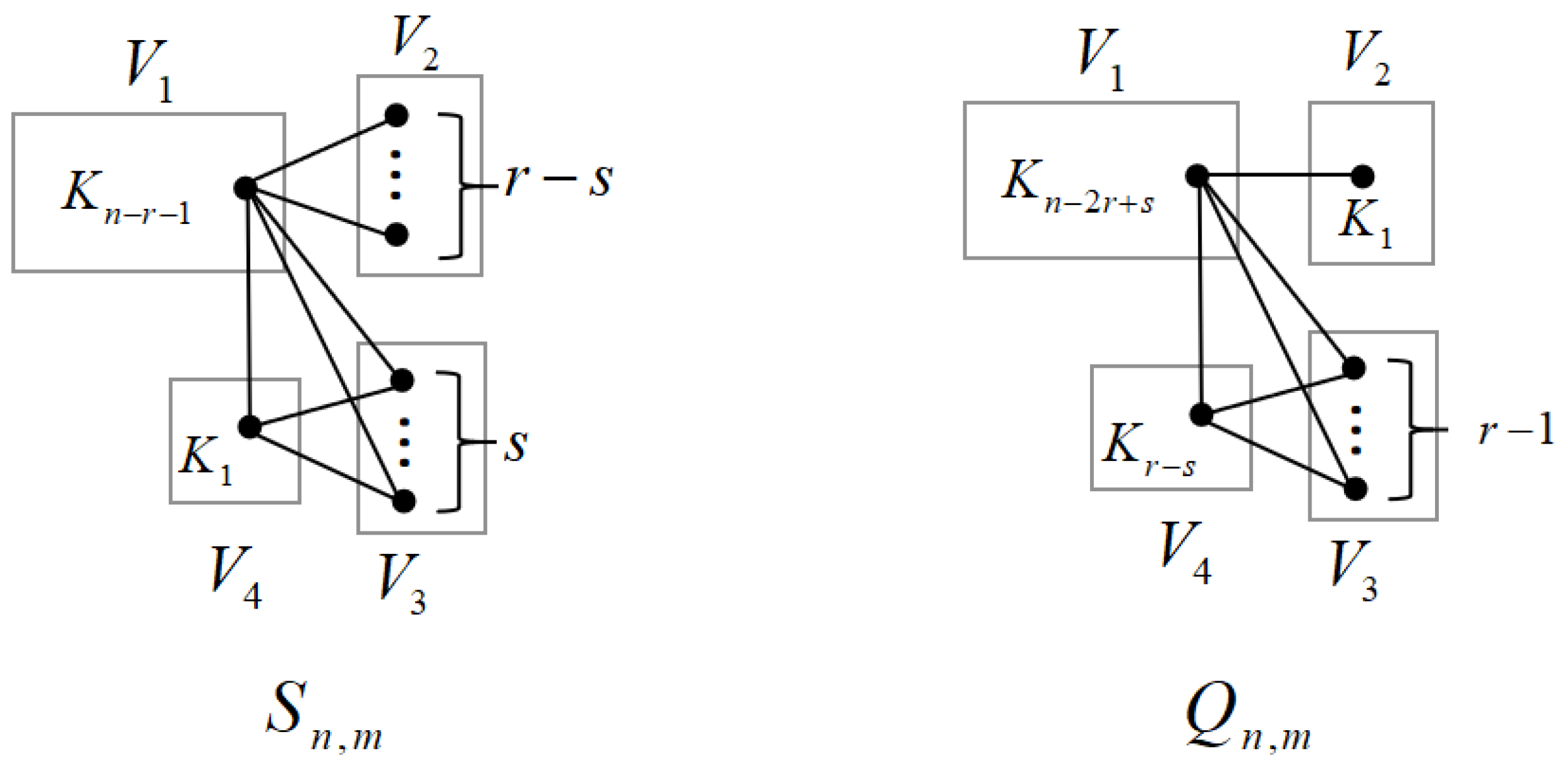
(1). We divide all vertices of into four parts:
: the vertices that are contained in the complete graph ;
: the vertices that are contained in the isolated vertices ;
: the vertices that are contained in the isolated vertices ;
: the unique isolated vertex (see Figure 1).
The number of triangles each of whose all vertices are contained in is , the number of triangles each of whose two vertices are contained in and one vertex is contained in is , the number of triangles each of whose two vertices are contained in and one vertex is contained in is , and the number of triangles each of whose two vertices are contained in and one vertex is contained in is . Besides, by a simple calculation, it can be seen that .
(2). We divide all vertices of into four parts:
: the vertices that are contained in the complete graph ;
: the unique isolated vertex ;
: the vertices that are contained in the isolated vertices ;
: the vertices that are contained in the complete graph (see Figure 1).
The number of triangles each of whose all vertices are contained in is , the number of triangles each of whose two vertices are contained in and one vertex is contained in is , the number of triangles each of whose two vertices are contained in and one vertex is contained in is . Besides, by a simple calculation, it can be seen that
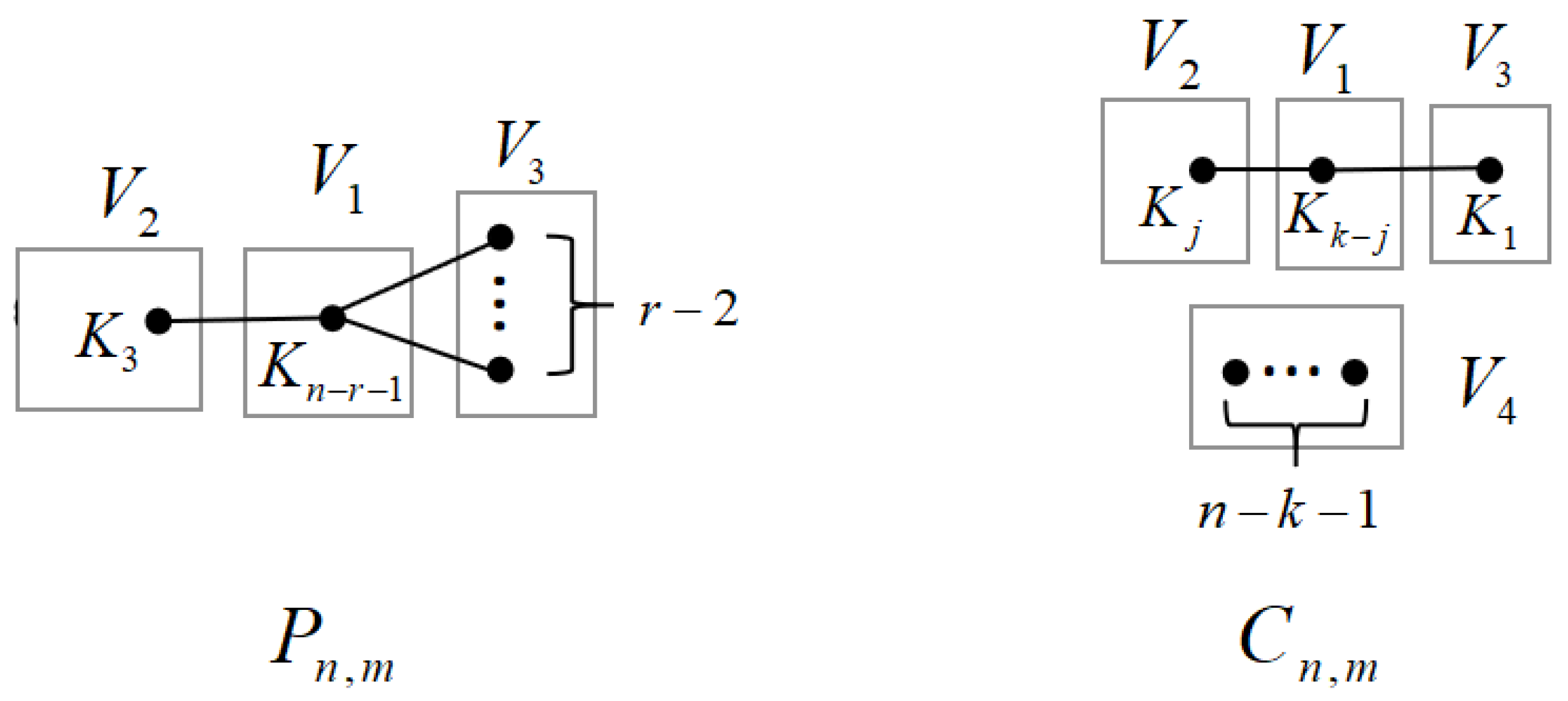
(3). We divide all vertices of into three parts:
: the vertices that are contained in the complete graph ;
: the vertices that are contained in the complete graph ;
: the vertices that are contained in the isolated vertices (see Figure 2).
The number of triangles each of whose all vertices are contained in is , the number of triangles each of whose two vertices are contained in and one vertex is contained in is . So
(4). We divide all vertices of into four parts:
: the vertices that are contained in the complete graph ;
: the vertices that are contained in the complete graph ;
: the isolated vertex ;
: some isolated vertices (see Figure 2).
The number of triangles each of whose all vertices are contained in is , the number of triangles each of whose two vertices are contained in and one vertex is contained in is . The number of triangles each of whose all vertices are contained in is , the number of triangles each of whose two vertices are contained in and one vertex is contained in is . The number of triangles each of whose two vertices are contained in and one vertex is contained in is . Besides, by a simple calculation, it can be seen that So .
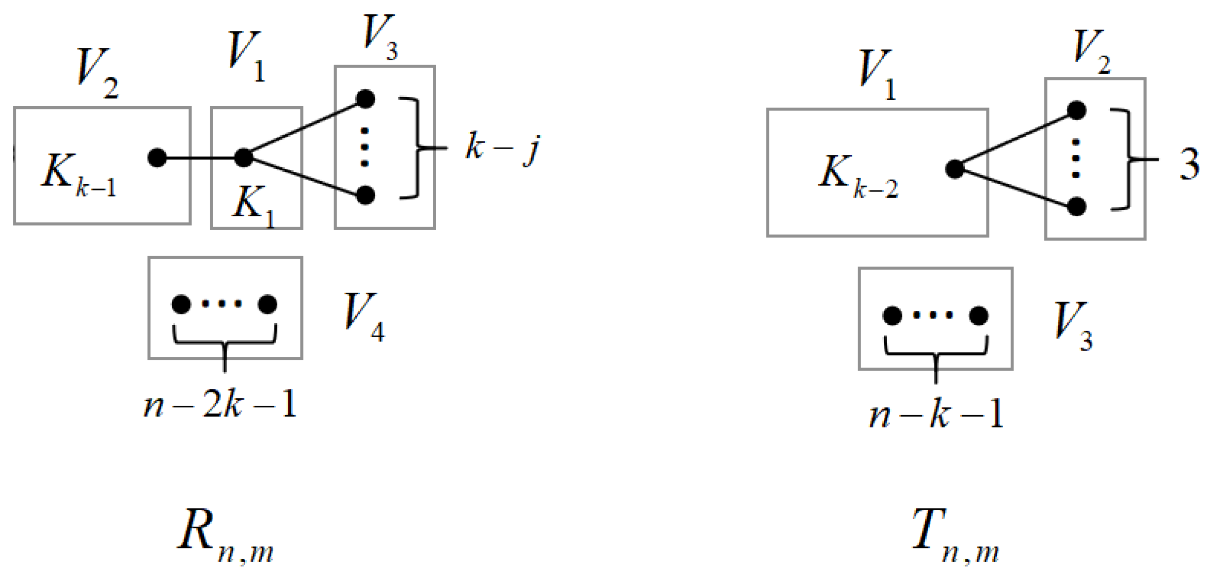
(5). We divide all vertices of into four parts:
: one vertex ;
: the vertices that are contained in the complete graph ;
: some isolated vertices ;
: some isolated vertices (see Figure 3).
The number of triangles each of whose all vertices are contained in is , the number of triangles each of whose two vertices are contained in and one vertex is contained in is . Besides, by a simple calculation, it can be seen that So .
(6). We divide all vertices of into three parts:
: the vertices that are contained in the complete graph ;
: three isolated vertices ;
: some isolated vertices (see Figure 3).
The number of triangles each of whose all vertices are contained in is , the number of triangles each of whose two vertices are contained in and one vertex is contained in is . Besides, by a simple calculation, it can be seen that So .
Therefore, the proof is complete. □
Now we establish two main theorems as follows. These theorems can help us better identify the candidate graphs of - minimal successive graphs in .
Theorem 3.
Let be a given integer pair with . Then
- (1).
- if and are -minimal;
- (2).
- if and are -minimal;
- (3).
- if and are -minimal;
- (4).
- if and are -minimal.
Proof.
Combining with the degree sequences above and Lemma 2, we have
(1). By a direct calculation, as .
(2). as . So (1) and (2) are trivial.
(3). Note that , we define
Recall that , then and thus the derivative satisfies which implies that is an increasing function on r. Consequently, . Thus (3) follows.
(4). Note that , we define
a function on k. Recall that , then and thus the derivative satisfies which implies that is a decreasing function on k. Consequently, . Thus (4) follows. □
In the following theorem, we exclude the rare case of , and .
Theorem 4.
Let be a given integer pair with . Then
- (1).
- if and are -minimal;
- (2).
- if and are -minimal;
- (3).
- and if and are -minimal.
Proof.
(1). Note that , we define
a function on n. Recall that and thus the derivative satisfies . We define . Recall that and , , then and thus the first derivative satisfies which implies that is a decreasing function on k. , which implies that is an increasing function on n. If , then . Consequently, . Thus (1) follows.
(2). Since integer satisfies the Pell’s equation , integer n is at least 12, and at the same time , . Note that , we define
The derivative satisfies
The second derivative satisfies
The third derivative satisfies
which implies that is an increasing function on n. , which implies that is an increasing function on n. , which implies that is an increasing function on n. Consequently, . Thus (2) follows.
(3). By Lemma 3 (6), if and are all optimal, then or , and also exists. Substituting into Equations (1) and (2) yields , , , and . By further direct calculation, , and . Similarly, substituting into Equations (1) and (2) yields and . By further direct calculation, , and . It is not difficult to see that is always the smallest. □
5. Results
By Theorem 4 and Lemma 3 (6), if and are -minimal, then also exists, and is - successive minimal.
By Lemma 3, Proposition 1 and Theorem 3, at least one of and be a - successive minimal graph in . or can only be a - successive minimal graph if certain conditions are satisfied, while or cannot be - successive minimal graph. Therefore, we have the main results of the paper as follows.
Theorem 5.
Let . If , or with or with , the - successive minimal graph is .
Theorem 6.
Let . If , or with , or with , each Laplacian coefficient - successive minimal graph is exactly one of the four classes of threshold graphs , , and .
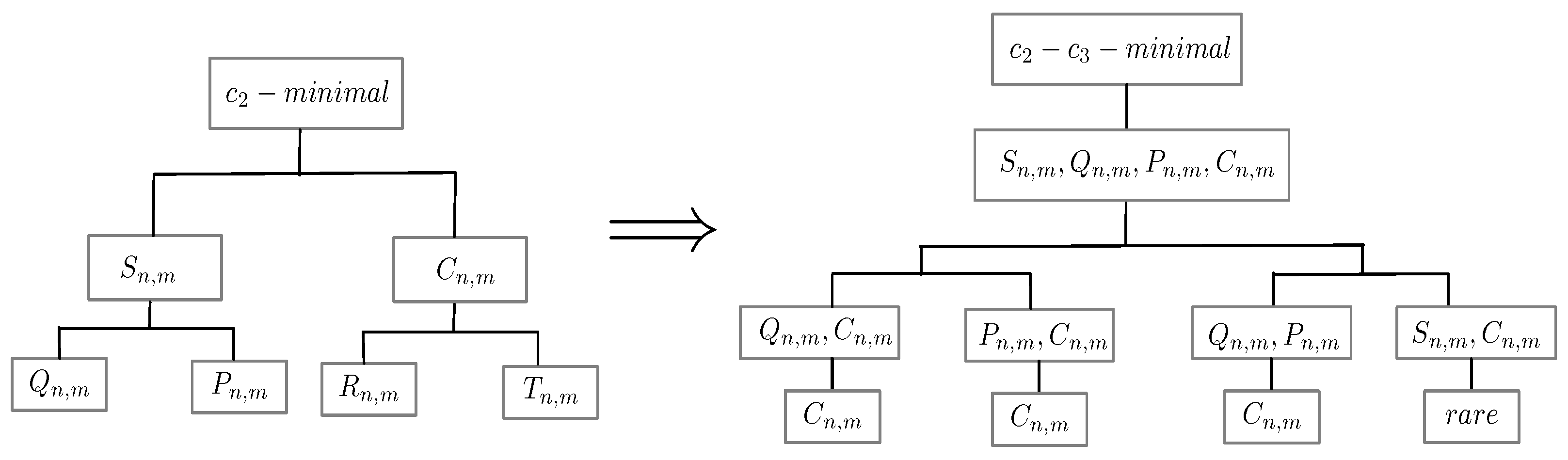
The Figure 5 describes the logical progression of our proofs.
Lemma 1 declares that the uniqueness of -minimal graphs cannot be guaranteed in . For instance, Theorem 2.5 in [31] demonstrates six -minimal graphs existing in . Theorems 3 and 4 further state that the - minimal successive graph in must be one of the four threshold graphs, that is, , , , and , with the exception that only and can be -minimal. Bearing in mind that for most integer pairs with , where the corresponding optimal -graph is unique, the -minimal graph is also unique. This being said, the cases where solely and are -minimal are infrequent and encompassed in Theorem 2.
After excluding the case where solely and are -minimal, we have successfully demonstrated the uniqueness of the - minimal successive graph in . However, it must be noted that this scenario is rarely encountered (as noted in Theorem 2, where the possibility of and both being -minimal is already uncommon). In light of this, we propose the conjecture that the - minimal successive graph in is indeed unique.
6. Conclusions
The research on the Laplacian matrix and its eigenvalues of graphs in the fields of physics and chemistry is notable. The coefficients of Laplacian matrix are directly linked to the eigenvalues and they serve as a reflection of the graph structure. In this paper, we extend Ábrego et al.’s work [31] and conduct a study of the - successive minimal graphs. Our research aims to gain a better understanding of the structural properties of molecular graphs.
Our next step is to map the threshold graph to the Ferrers matrix (the adjacency matrix of a threshold graph such that the upper-triangular part is left justified and the number of zeros in each row of the upper-triangular part does not decrease. We demonstrate Ferrers matrices using “+" for the main diagonal, an empty circle “∘" for the zero entries, and a black dot, “•" for the entries equal to one), attach weights corresponding to Laplacian coefficients to each element in the Ferrers matrix, and use a special perturbation of the threshold graph to minimize some Laplacian coefficients.
Author Contributions
Y.X.: Writing—original draft, Conceptualization, Writing—review & editing; S.-C.G.: Writing—review & editing, Supervision. All authors have read and agreed to the published version of the manuscript.
Funding
The authors gratefully acknowledge the financial support provided by the Natural Science Foundation of Zhejiang Province (LY20A010005), the National Natural Science Foundation of China (12271484), and Graduate Research and Innovation Fund of Zhejiang University of Science and Technology (2021yjskc21).
Data Availability Statement
Not applicable.
Conflicts of Interest
The authors declare no conflict of interest.
References
- Pan, Y.; Liu, C.; Li, J. Kirchhoff indices and numbers of spanning trees of molecular graphs derived from linear crossed polyomino chain. Polycycl. Aromat. Compd. 2021, 42, 218–225. [Google Scholar] [CrossRef]
- Klyukin, I.N.; Kolbunova, A.V.; Novikov, A.S. Theoretical Insight into B–C Chemical Bonding in Closo-Borate [BnHn−1CH3]2−(n=6,10,12) and Monocarborane [CBnHnCH3]−(n=5,9,11) Anions. Inorganics 2022, 10, 186. [Google Scholar] [CrossRef]
- Drake, R. Benchmark of Clustering Techniques and Potential Applications to Polymer Material Science; Liberty University: Lynchburg, VA, USA, 2022. [Google Scholar]
- Aliakbarisani, R.; Ghasemi, A.; Serrano, M.Á. Perturbation of the normalized Laplacian matrix for the prediction of missing links in real networks. IEEE Trans. Netw. Sci. Eng. 2021, 9, 863–874. [Google Scholar] [CrossRef]
- Cuadra, L.; Nieto-Borge, J.C. Modeling quantum dot systems as random geometric graphs with probability amplitude-based weighted links. Nanomaterials 2021, 11, 375. [Google Scholar] [CrossRef] [PubMed]
- Stevanović, D. Laplacian-like energy of trees. MATCH Commun. Math Comput. Chem. 2009, 61, 407. [Google Scholar]
- Mohar, B. On the Laplacian coefficients of acyclic graphs. Linear Algebra Appl. 2007, 722, 736–741. [Google Scholar] [CrossRef]
- Stevanović, D.; Ilić, A. On the Laplacian coefficients of unicyclic graphs. Linear Algebra Appl. 2009, 430, 2290–2300. [Google Scholar] [CrossRef]
- He, C.X.; Shan, H.Y. On the Laplacian coefficients of bicyclic graphs. Discret. Math. 2010, 310, 3404–3412. [Google Scholar] [CrossRef]
- Pai, X.Y.; Liu, S.Y.; Guo, J.M. On the Laplacian coefficients of tricyclic graphs. J. Math. Anal. Appl. 2013, 405, 200–208. [Google Scholar] [CrossRef]
- He, S.; Li, S. Ordering of trees with fixed matching number by the Laplacian coefficients. Linear Algebra Appl. 2011, 435, 1171–1186. [Google Scholar] [CrossRef]
- Ilić, A.; Ilić, M. Laplacian coefficients of trees with given number of leaves or vertices of degree two. Linear Algebra Appl. 2009, 431, 2195–2202. [Google Scholar] [CrossRef]
- Ilić, A. Trees with minimal Laplacian coefficients. Comput. Math. Appl. 2010, 59, 2776–2783. [Google Scholar] [CrossRef]
- Ilić, A. On the ordering of trees by the Laplacian coefficients. Linear Algebra Appl. 2009, 431, 2203–2212. [Google Scholar] [CrossRef]
- Ilić, A.; Ilić, A.; Stevanović, D. On the Wiener index and Laplacian coefficients of graphs with given diameter or radius. MATCH Commun. Math. Comput. Chem. 2010, 63, 91–100. [Google Scholar]
- Lin, W.; Yan, W.G. Laplacian coefficients of trees with a given bipartition. Linear Algebra Appl. 2011, 435, 152–162. [Google Scholar] [CrossRef]
- Tan, S.W. On the Laplacian coefficients of unicyclic graphs with prescribed matching umber. Discret. Math. 2011, 311, 582–594. [Google Scholar] [CrossRef]
- Tan, S.W.; Song, T.M. On the Laplacian coefficients of trees with a perfect matching. Linear Algebra Appl. 2012, 436, 595–617. [Google Scholar] [CrossRef]
- Zhang, X.D.; Lv, X.P.; Chen, Y.H. Ordering trees by the Laplacian coefficients. Linear Algebra Appl. 2009, 431, 2414–2424. [Google Scholar] [CrossRef]
- Ahlswede, R.; Katona, G.O.H. Graphs with maximal number of adjacent pairs of edges. Acta Math. Acad. Sci. Hungar. 1978, 32, 97–120. [Google Scholar] [CrossRef]
- Cutler, J.; Radcliffe, A.J. Extremal graphs for homomorphisms. J. Graph. Theory 2011, 67, 261–284. [Google Scholar] [CrossRef]
- Mahadev, N.V.R.; Peled, U.N. Threshold Graphs and Related Topics, 1st ed.; Elsevier: Amsterdam, The Netherlands, 1995; pp. 7–32. [Google Scholar]
- Keough, L.; Radcliffe, A.J. Graphs with the fewest matchings. Combinatorica 2016, 36, 703–723. [Google Scholar] [CrossRef]
- Gong, S.C.; Zou, P.; Zhang, X.D. Each (n,m)-graph having the i-th minimal Laplacian coefficient is a threshold graph. Linear Algebra Appl. 2021, 631, 398–406. [Google Scholar] [CrossRef]
- Katz, M. Rearrangements of (0–1) matrices. Isr. J. Math. 1971, 9, 13–15. [Google Scholar] [CrossRef]
- Gutman, I. Degree based topological indices. Croat. Chem. Acta. 2013, 86, 351–361. [Google Scholar] [CrossRef]
- Gutman, I. On the origin of two degree based topological indices. Bull. Acad. Serbe Sci. Arts (Cl. Sci. Math. Natur.) 2014, 146, 39–52. [Google Scholar]
- Oliveira, C.S.; Abreu, N.; Jurkiewicz, S. The characteristic polynomial of the Laplacian of graphs in (a,b)-linear classes. Linear Algebra Appl. 2002, 356, 113–121. [Google Scholar] [CrossRef]
- Peled, U.N.; Petreschi, R.; Sterbini, A. (n;e)-graphs with maximum sum of squares of degrees. J. Graph. Theory. 1999, 31, 283–295. [Google Scholar] [CrossRef]
- Byer, O.D. Two path extremal graphs and an application to a Ramsey-type problem. Discret. Math. 1999, 196, 51–64. [Google Scholar] [CrossRef]
- Ábrego, B.M.; Fernández-Merchant, S.; Neubauer, M.G.; Watkins, W. Sum of squares of degrees in a graph. Inequal. Pure Appl. Math. 2009, 10, 64. [Google Scholar]
- Gong, S.C.; Zhang, L.P.; Su, C.B. On the Number of All Substructures Containing at Most Four Edges. MATCH Commun. Math Comput. Chem. 2023, 89, 327–342. [Google Scholar] [CrossRef]
Figure 1.
, .

Figure 2.
, .

Figure 3.
, .

Figure 4.
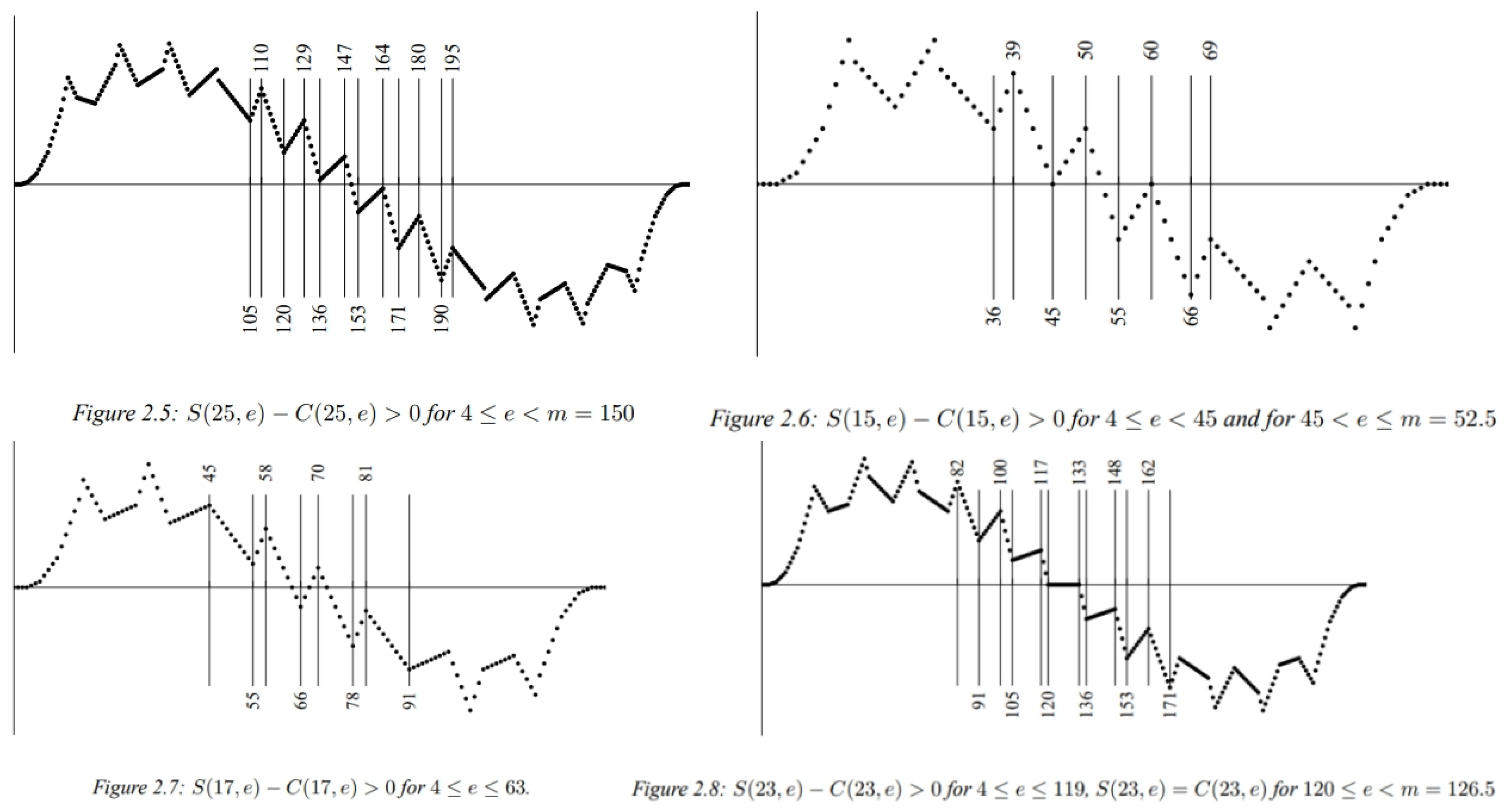
In reference [31], . and e denote the sum of squares of degrees and the number of edges of the quasi-star graph.
Figure 4.
In reference [31], . and e denote the sum of squares of degrees and the number of edges of the quasi-star graph.

Figure 5.
Only when is -minimal graph, and can be -minimal graphs. Similarly, only when is -minimal graph, and can be -minimal graphs. The application of Theorem 3 enables us to reduce the set of candidate graphs for - successive minimal graphs to four types of threshold graphs, namely: , , and . Besides, Theorem 4 indicates that, if with with , the - successive minimal graph is .

Disclaimer/Publisher’s Note: The statements, opinions and data contained in all publications are solely those of the individual author(s) and contributor(s) and not of MDPI and/or the editor(s). MDPI and/or the editor(s) disclaim responsibility for any injury to people or property resulting from any ideas, methods, instructions or products referred to in the content. |
© 2023 by the authors. Licensee MDPI, Basel, Switzerland. This article is an open access article distributed under the terms and conditions of the Creative Commons Attribution (CC BY) license (https://creativecommons.org/licenses/by/4.0/).
Share and Cite
MDPI and ACS Style
Xu, Y.; Gong, S.-C. On Graphs with c2-c3 Successive Minimal Laplacian Coefficients. Axioms 2023, 12, 464. https://doi.org/10.3390/axioms12050464
AMA Style
Xu Y, Gong S-C. On Graphs with c2-c3 Successive Minimal Laplacian Coefficients. Axioms. 2023; 12(5):464. https://doi.org/10.3390/axioms12050464
Chicago/Turabian StyleXu, Yue, and Shi-Cai Gong. 2023. "On Graphs with c2-c3 Successive Minimal Laplacian Coefficients" Axioms 12, no. 5: 464. https://doi.org/10.3390/axioms12050464
Note that from the first issue of 2016, this journal uses article numbers instead of page numbers. See further details here.