Sustainable Supply Chain Model for Defective Growing Items (Fishery) with Trade Credit Policy and Fuzzy Learning Effect

Abstract

Fundamentally, newborn items that are used commercially, such as chicken, fish, and small camel, grow day by day in size and also increase their weight. The seller offers a credit policy to the buyer to increase sales for a particular growing item (fish), and in this paper, it is assumed that the buyer accepts the policy of the trade credit. In this paper, the buyer acquires the newborn items (fish) from the seller and then sells them when the newborn items have increased their size and weight. From this point of view, the present paper reveals a fuzzy-based supply chain model that includes carbon emissions and a permissible delay in payment for defective growing items (fish) under the effect of learning where the demand rate is imprecise in nature and is treated as a triangular fuzzy number. Finally, the buyer’s total profit is optimized with respect to the number of newborn items. A numerical example has been presented for the justification of the model. The findings clearly suggest that the presence of trade credit, learning, and a fuzzy environment have an affirmative effect on the ordering policy. The buyer should order more to avoid higher interest charges after the grace period, which eventually increases their profit, while at the same time, it is also beneficial for the buyer to order less to gain the benefit of the trade credit period. The fuzziness theory controls the uncertainty situation of inventory parameters with the help of a de-fuzzified method. The lower and upper deviation of demand affects the total fuzzy profit. The effect of learning gives a positive response concerning the size of the order and the buyer’s total fuzzy profit. This means that the decision-maker should be aware of the size of the newborn items, rate of learning, and trade credit period during the supply chain because these directly affect the buyer’s total fuzzy profit. The impact of the inventory parameter of this model is presented with the help of sensitivity analysis.

1. Introduction

This section covers the literature review studies that form the background of the proposed study and includes an introduction to the proposed study.

1.1. Literature Review According to the Trade-Credit Policy Model under Various Policies

Supply chain management is a good tool for businesses, industries, firms, etc., and involves stock inventory management. Many researchers relatively worked on supply chains with various strategies for different items. Harris [1] presented the first inventory model in 1913 for an ordering policy for deteriorating items. A significant amount of inventory models have been extended using the theory of this initial model, with various approaches for perishable items or deteriorating items or vegetables, but we have selected a few literature reviews relative to this paper study. Aggarwal and Jaggi [2] developed a new model with a credit period for deteriorating items and achieved positive effects on the total profit. Chu et al. [3] defined a strategy for the credit period for deteriorating items. Abad and Jaggi [4] considered an inventory model with the help of a credit-period policy for the deterioration of items, where the demand rate was a function of the selling price, and calculated the length of the credit period, which is the most important element for both players.

1.2. Literature Review According to the Trade-Credit Policy and Imperfect Quality Items-Based Model under Various Policies

Chung and Liao [5] presented an imperfect quality-based inventory model with decaying items for the ordering strategy, where the seller offers a credit period to his buyer, and both players acquire more profit. Salameh and Jaber [6] proposed a model with imperfect quality items under a screening process. Chung et al. [7], inspired by the model of Chung and Lia [5], proposed an imperfect quality-based model for the two-warehouse system. Various researchers, such as Huang [8], Jaber et al. [9], and Jaggi et al. [10], have worked on imperfect items with various policies.

1.3. Literature Review According to the Imperfect Quality Items, Carbon Emissions, and Growing Items-Based Model under Various Policies

Carbon emissions from different sources are very harmful to the environment. An important number of authors have presented models for various strategies regarding carbon emissions from imperfect quality items. Zhang et al. [11] presented a new policy model with growing items regarding carbon emissions, where the amount of carbon emissions was calculated. Tiwari et al. [12] presented a carbon emissions-based model with defective quality items for deteriorating items. Sebatjane and Adetunji [13] proposed an EOQ model with defective products for growing items, calculated the expected total profit for the supply chain under the logistic growth function and split linear. De-la-Cruz-Marquez et al. [14] described a mathematical model for growing defective quality items under the effects of shortages and carbon emissions, where the demand rate depended on the selling price.

1.4. Literature Review According to Imperfect Quality Items, Carbon Emissions, Trade Credit, and Learning Fuzzy Theory-Based Model under Various Policies

Most researchers consider the rate of demand as imprecise in nature. In this way, Chang [15] proposed an EOQ model with defective quality items under a fuzzy environment. Rani et al. [16] discussed a fuzzy-based inventory model with carbon emissions for deteriorating items under a green supply chain. The concept of learning has been presented by Wright [17] in the field of inventory, which suggested that some factors affect the total inventory cost. Wee and Chen [18] proposed an economic order quantity model for defective items under the effect of shortages. Jayaswal et al. [19] presented an EPQ model under the effect of learning under the credit period. Jayaswal et al. [20] proposed an EOQ model for defective quality items regarding the effect of leaning under a credit period scheme. Alamri et al. [21] proposed an EOQ model with inflation and carbon emissions under the effect of learning for deteriorating items. Jayaswal et al. [22] presented an EOQ model regarding the effect of a leaning and credit financing policy under a cloudy fuzzy environment.

1.5. Introduction of the Proposed Study

The present paper deals with a seller–buyer model in which the seller provides newborn growing items (when the weight of the newborn items is raised) to the buyer under a credit policy, where the demand rate is imprecise in nature and treated as a triangular fuzzy number. The seller offers a credit policy scheme to the new client for the increased sale of newborn growing items, which, therefore, generates more revenue. Often, buyers do not have adequate money revenue to conduct business and, therefore, accept the trade credit scheme, which bounds them to multiply more effort in generating sales. When the buyer receives a lot of newborn growing items and has inspected the whole lot with a constant inspection rate, he divides the whole lot into two parts: non-defective and defective. The buyer sells the defective items at a low price and none defective items at a higher price. In this model, the buyer assumes that defective items follow the effect of the learning curve and includes some carbon emission cost due to holding units. Finally, the total fuzzy profit is optimized with respect to the number of newborn growing items and de-fuzzified with the help of the signed distance method. The research gap and our research study are shown in the next paragraph.

1.5.1. Introduction of the Proposed Study’s Background, Perspective, Research Gap, and Our Contribution

As mentioned above, it can clearly be seen that little attention was paid to managing growing items (fishes) during the business deal. We tried to promote a sustainable supply chain model with carbon emissions and learning effects under a fuzzy environment and trade credit scheme in which the supply chain players get more profit under some realistic situation. Basically, the present study has been developed for the fishery where sellers purchase newborn growing items and then sometimes sell them when the weight of the newborn items is raised. We have discussed a few relatable literature articles that synchronize with the present study’s background, such as Rezaei [23], which presented an inventory model for the growing items where the demand rate has been taken as a linear function. In this order, Sebatjane and Adetunji [13] developed a mathematical model for the growing items with imperfect quality items. Mittal and Sharma [24] proposed a growing items-based inventory model under a credit scheme. Renowned authors such as Rezaei [23], Sebatjane and Adetunji [13], and Mittal and Sharma [24] were not oriented toward the application of the learning curve, fuzzy theory as well as carbon emissions concept. We were motivated by the study of Mittal and Sharma [24] and from the literature review of Jayaswal et al. [25] to Rajeswari et al. [26], and their contributions have been described in

Table 1. Description of the author’s contribution, research gap, and present study.

Authors	Imperfect Quality Items	Growing Items	Trade Credit Policy	Carbon Emissions	Learning Effect	Fuzzy Environment
Wright [17]					🗸
Salameh and Jaber [6]	🗸
Jaber et al. [9]	🗸				🗸
Sebatjane and Adetunji [13]	🗸	🗸
Mittal and Sharma [24]		🗸	🗸
Jayaswal et al. [19]	🗸		🗸		🗸	🗸
Alamri et al. [21]	🗸			🗸	🗸
Jayaswal et al. [22]	🗸		🗸		🗸	🗸
Rezaei [23]		🗸
Mittal and Sharma [24]	🗸	🗸	🗸
Pattnaik [25]	🗸					🗸
Rajeswari et al. [26]						🗸
Mahapatra et al. [27]					🗸	🗸
Taheri and Mirzazadeh [28]					🗸	🗸
Dinagar and Manvizhi [29]	🗸					🗸
Garg et al. [30]	🗸					🗸
Kuppulakshmi et al. [31]	🗸					🗸
Jayaswal and Mittal [32]	🗸		🗸			🗸
Chung and Huang [33]	🗸		🗸
Sulak [34]	🗸					🗸
Shekarian et al. [35]	🗸				🗸	🗸
Kazemi et al. [36]	🗸			🗸
Present study	🗸	🗸	🗸	🗸	🗸	🗸

. The present study tried to fill the research gap using the concept of learning, credit scheme, fuzzy concept, and carbon emissions. We considered some selected research work related to our work, as included in Table 1. Table 1 is treated as a contribution of authors-related research work, and in the end, our work will be justified. We assumed the inventory problem in which demand for newborn items is considered a fuzzy variable to handle the uncertainty of the market. The present study helps decision-makers to make more stable decisions in an uncertain environment. It is also evident that the learning process will facilitate decision-makers in their decision-making prerogatives, which helps bring about higher profit. We have discussed the subsequent realistic problems in our proposed model:

(i)

How buyer’s total fuzzy profit and order quantity get affected by trade credit policy under fuzzy environment.

(ii)

What is the impact of the learning rate on the buyer’s total fuzzy profit under a fuzzy environment?

(iii)

What is the impact of the number of shipments on the buyer’s total fuzzy profit under a fuzzy environment?

(iv)

How the buyer’s total fuzzy profit gets affected by changes in various parameters (distance, feeding cost, ordering cost, selling price, etc.).

(v)

How the buyer’s total fuzzy profit gets affected by changes in lower and upper deviation of demand rate.

The contribution made by the researcher in the present paper is the inclusion of trade credit policy and learning fuzzy theory for the growing items (Fishery) shown at the bottom in Table 1.

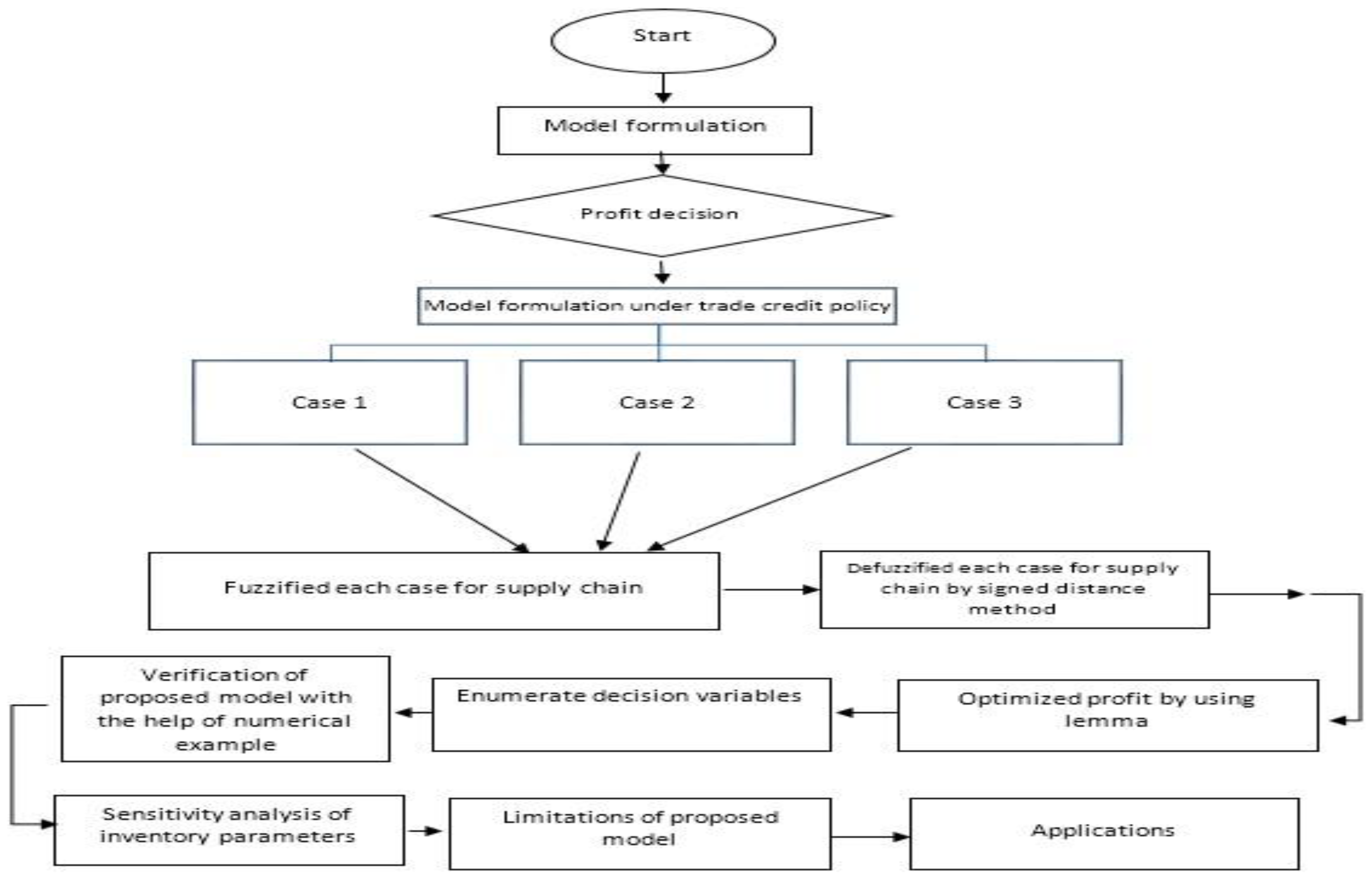
1.5.2. Outlook of Present Study through Flowchart

The presentation of the flowchart is a short review of any proposed work. We tried to summarize the methodology of the proposed study through a flowchart, as shown in Figure 1.

2. Assumptions and Definitions

2.1. Assumption

The following assumptions have been considered in this paper and are given below:

⮚

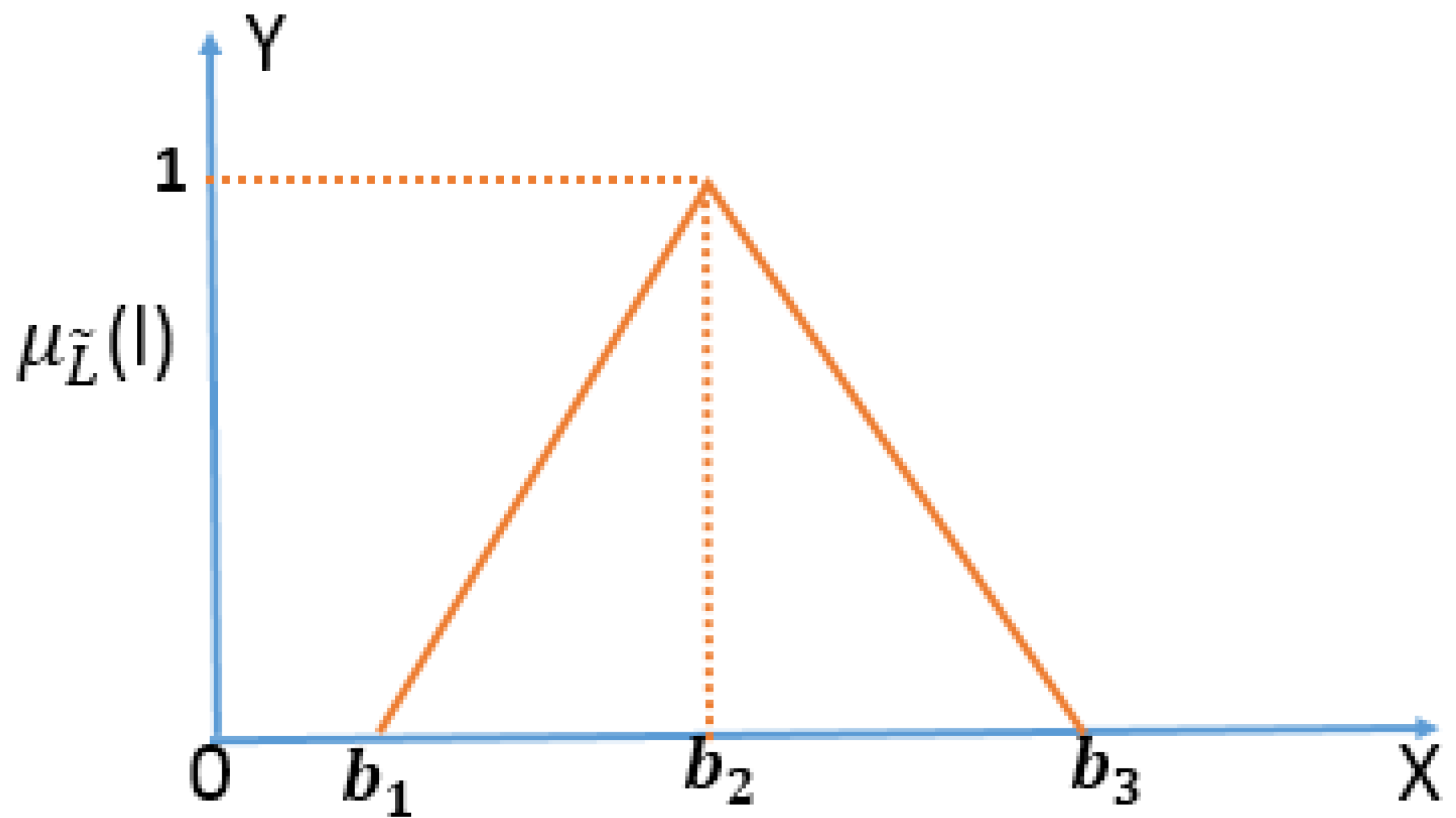
The demand rate has been considered imprecise in nature and treated as a triangular fuzzy number (Alsaedi et al. [37]). The triangular fuzzy number is used to fuzzify the model, and the signed distance method is applied to defuzzify the model.

⮚

Let us consider that the seller provides growing items to the buyer, and the lot has some defective growing items (Sebatjane and Adetunji [13]). It is also assumed that the seller offers a trade credit period to the buyer, and the buyer accepts the policy of trade credit (Aggarwal and Jaggi [2]).

⮚

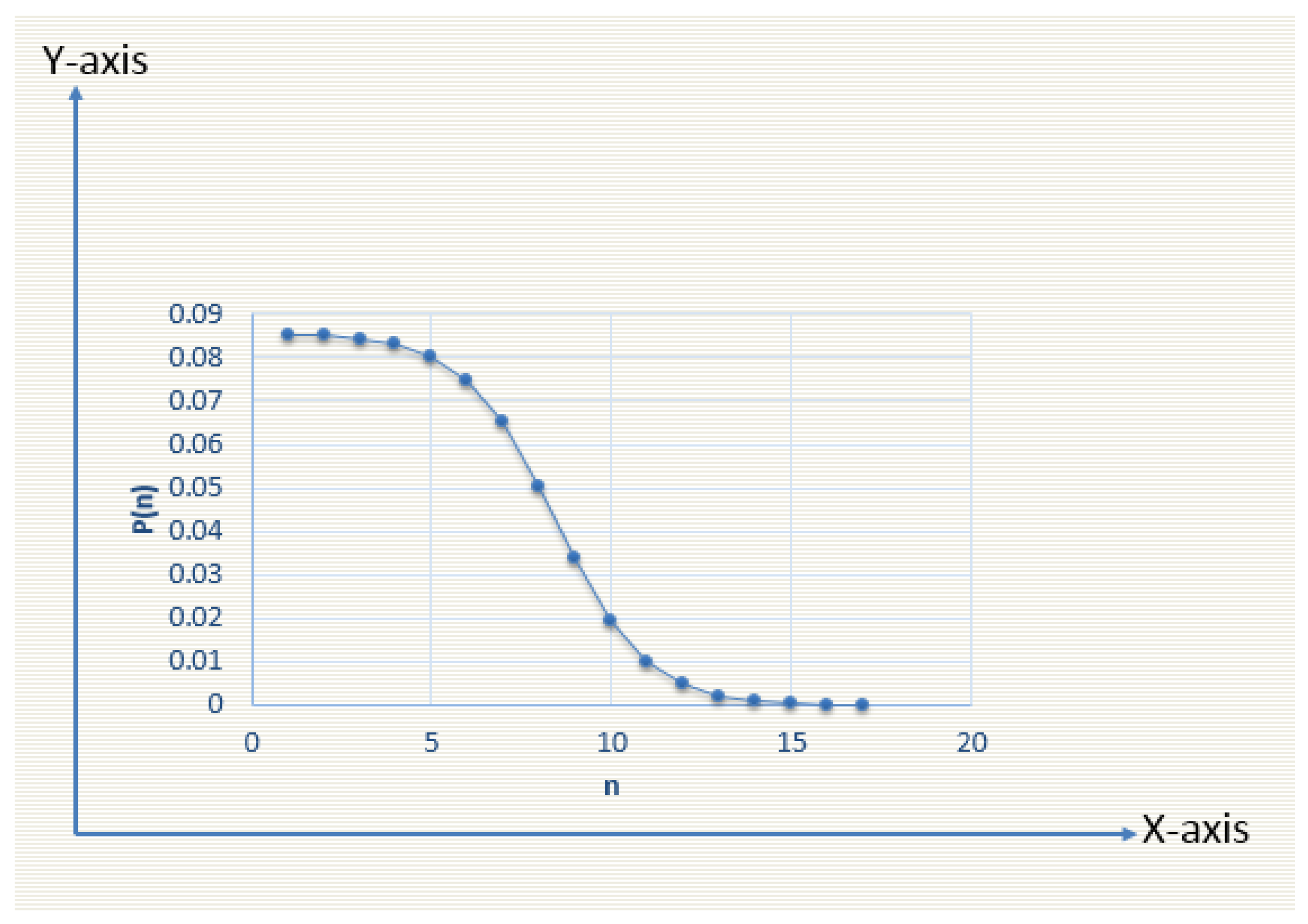
It is assumed that the buyer inspects the whole lot received at a constant screening rate; after that, the buyer separates the whole lot received from the seller into two categories, defective and non-defective items, and then sells them at different selling prices (Salameh and Jaber [6]). It is also considered that the selling price of good quality is greater than that of defective quality items (poorer) (Jaggi et al. [38]). The fraction of defective growing items follows the S-shape learning curve (Jaber et al. [9]). All defective growing items are sold in different markets (Mittal and Sharma [24]).

⮚

To avoid shortages within screening time.

⮚

It is assumed that the rework or lack of replacement of growing defective items after the delivery of the lot.

⮚

The demanded items are capable of growing prior to being slaughtered (Sebatjane and Adetunji [13]) and include the feeding cost. The cost of feeding the items is proportional to the weight gained by the items (Mittal and Sharma [24]).

⮚

It is supposing that when the transaction of the newborn items shifts from one place to another, a lot of carbon units emit due to transportation, which is very harmful to the environment and incorporates emission cost for low carbon units (Guru et al. [39]).

2.2. Some Basic Definitions

Below are some useful definitions required for developing the present paper.

Definition 1.

Suppose that if the universal set is $S$ and any set $L$ on $S$, the fuzzy set can be defined on $S$ and it is mentioned by $\tilde{L}$ and where $\tilde{L}=\left\{\left(l, {\mu }_{\widetilde{ L}}{}_{ }\left(\tilde{l}\right)\right):l\in S\right\}$, ${\mu }_{\widetilde{ L}}$ is a membership function that is defined from $S$ to [0,1]. If the three numbers with the condition $b_1<b_2<b_3$, then the triplet $\left(b_1,b_2,b_3\right)$ are known as triangular fuzzy numbers; if their membership function will be

$${\mu }_{\tilde{L}}=\{\begin{array}{c}\frac{b-b_1}{b_2-b_1} b\in {\left[b_1,b_2 \right]}_{ }\\ \frac{b_3-b}{b_3-b_2} b\in {\left[b_2,b_3 \right]}_{ }\\ 0 \mathrm{Otherwise}\end{array}$$

Definition 2.

If we take any number, let us say, $z$ and $0\in S$, then the signed distance can be calculated from the number $z$ to $0$, which can be represented by $d\left(z,0\right)=z$ and also for the negative of any number, the signed distance from $\left(-z\right)$ to 0, we can represent it such that $d\left(-z,0\right)=-z$ where the negative sign represents the direction of $z$ and it will be in the opposite direction of positive $z.$ It is considered that Ω is the collection of fuzzy sets $\tilde{Z}$, which is defined on $S$. The $\alpha -cut,$ $Z\left(\alpha \right)=\left[Z_L\left(\alpha \right),Z_U\left(\alpha \right)\right],exits$ $\forall \alpha \in \left[0.1\right]$ then $Z\left(\alpha \right)=\left[Z_L\left(\alpha \right),Z_U\left(\alpha \right)\right]$, $Z_L\left(\alpha \right) and Z_U\left(\alpha \right)$ are the continuous function and defined on $\alpha$. The $\alpha -cut,$ $Z\left(\alpha \right)$ can be represented by $Z\left(\alpha \right)={{\displaystyle \cup }}_{0\ll \alpha \ll 1}\left[Z_L{\left(\alpha \right)}_{\alpha }, Z_U{\left(\alpha \right)}_{\alpha }\right]$.

Definition 3.

It is supposed that, $\tilde{Z}$$\in$ Ω, then the signed distance of $\tilde{Z}$ from ${\tilde{0}}_1$ can be defined below

$$d\left(z,0\right)=\frac{{{\displaystyle \int }}_0^1\left[Z_L\left(\alpha \right)+Z_U\left(\alpha \right)\right]d\alpha }{2}$$

(1)

Definition 4.

If $\tilde{Z}=\left(z_1,z_2,z_3\right)$ represents the triangular fuzzy number, then $\alpha -cut$ of $\tilde{Z}$ is $Z\left(\alpha \right)=\left[Z_L\left(\alpha \right),Z_U\left(\alpha \right)\right]$, where $Z_L\left(\alpha \right)=z_1+\left(z_2-z_1\right)\alpha$ and $C_U\left(\alpha \right)=z_3-\left(z_1-z_2\right)\alpha$. The signed distance of $\tilde{Z}$ to ${\tilde{0}}_1$ is

$$d\left(\widetilde{ Z},0\right)=\frac{\left(z+2z_2+z_3\right)}{2}$$

(2)

3. Model Formulation

3.1. S-Shape Learning Curve

The effects of learning operate as a significant function for reducing the inventory cost and also optimizing the total profit of the inventory system. Figure 2 graphically represents the S-shape learning curve with the help of the given data below and in the form of a formula (Jaber et al. [9]) $P\left(n\right)=\frac{a}{g+e^{bn}}, a>0, g>0,$ where $b$ represents the parameter of learning and $n$ is a shipment (shown in Figure 3).

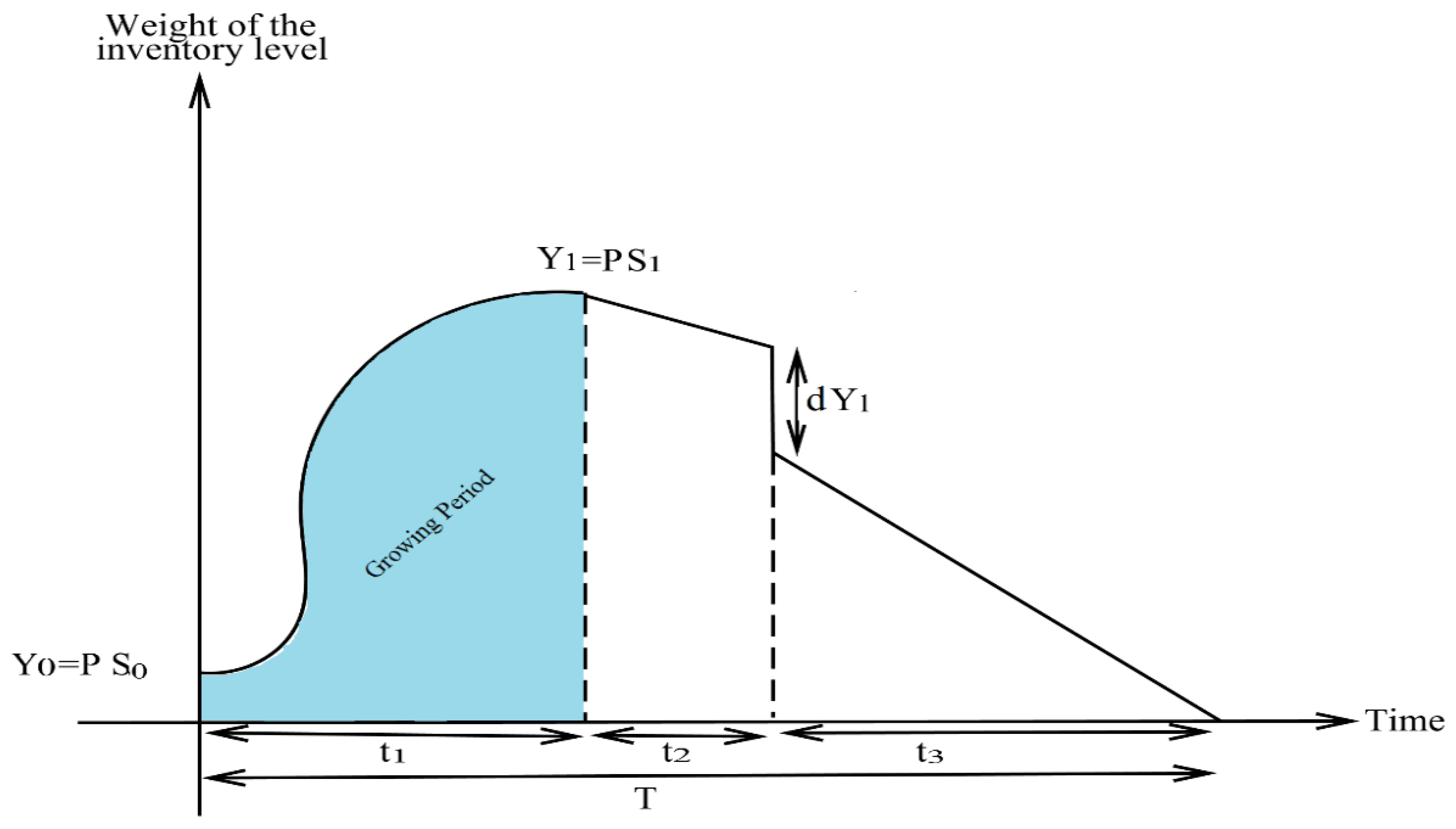
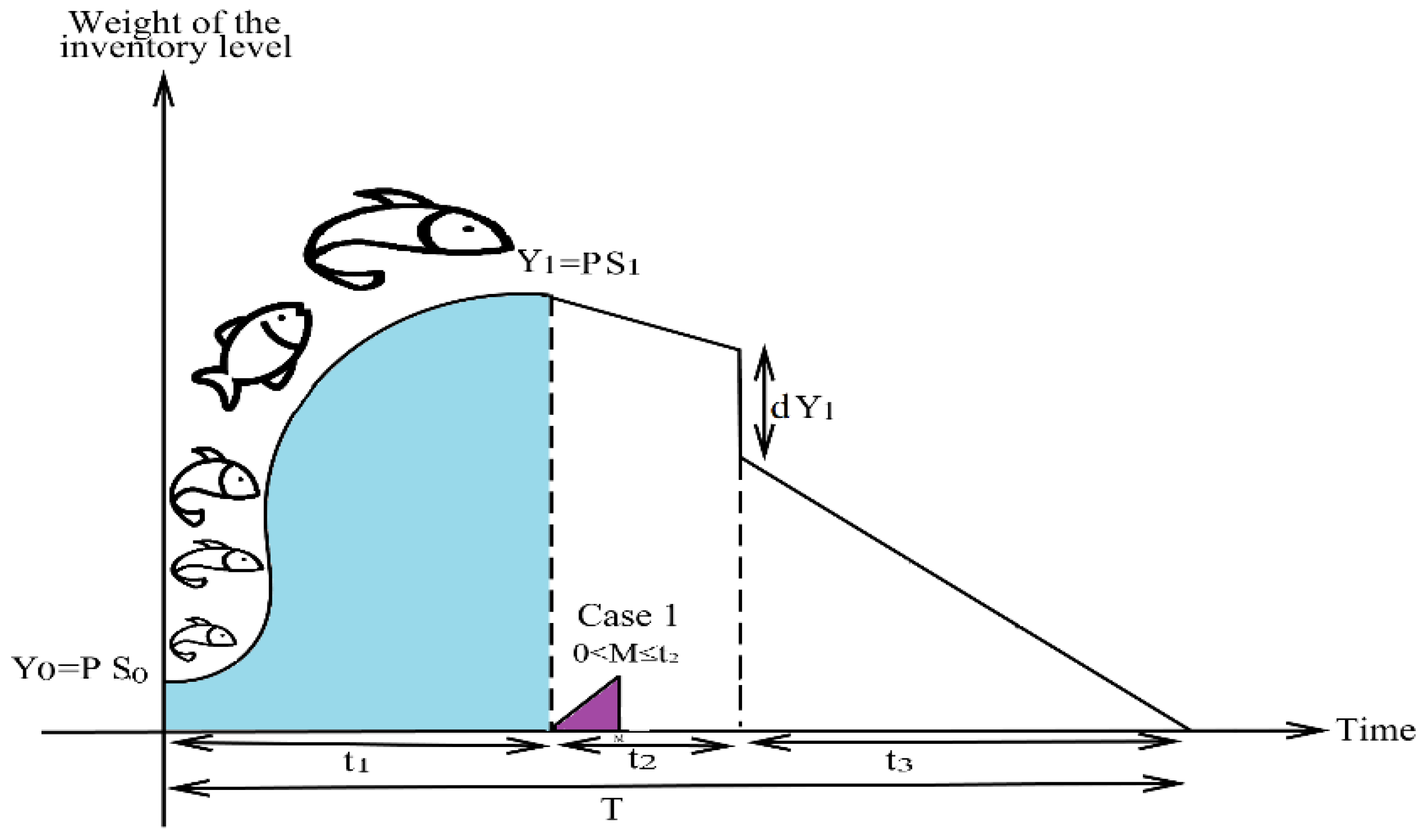
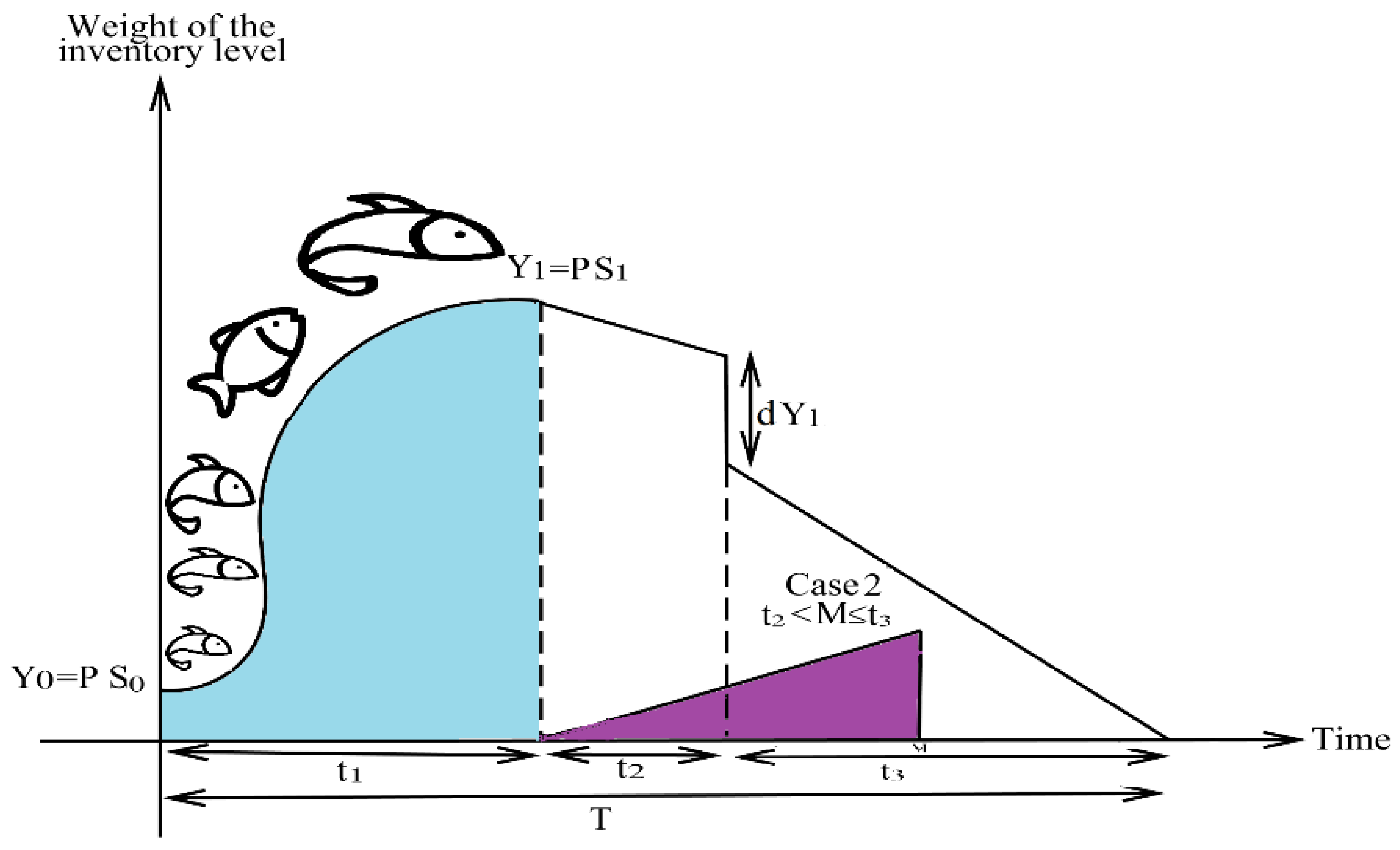
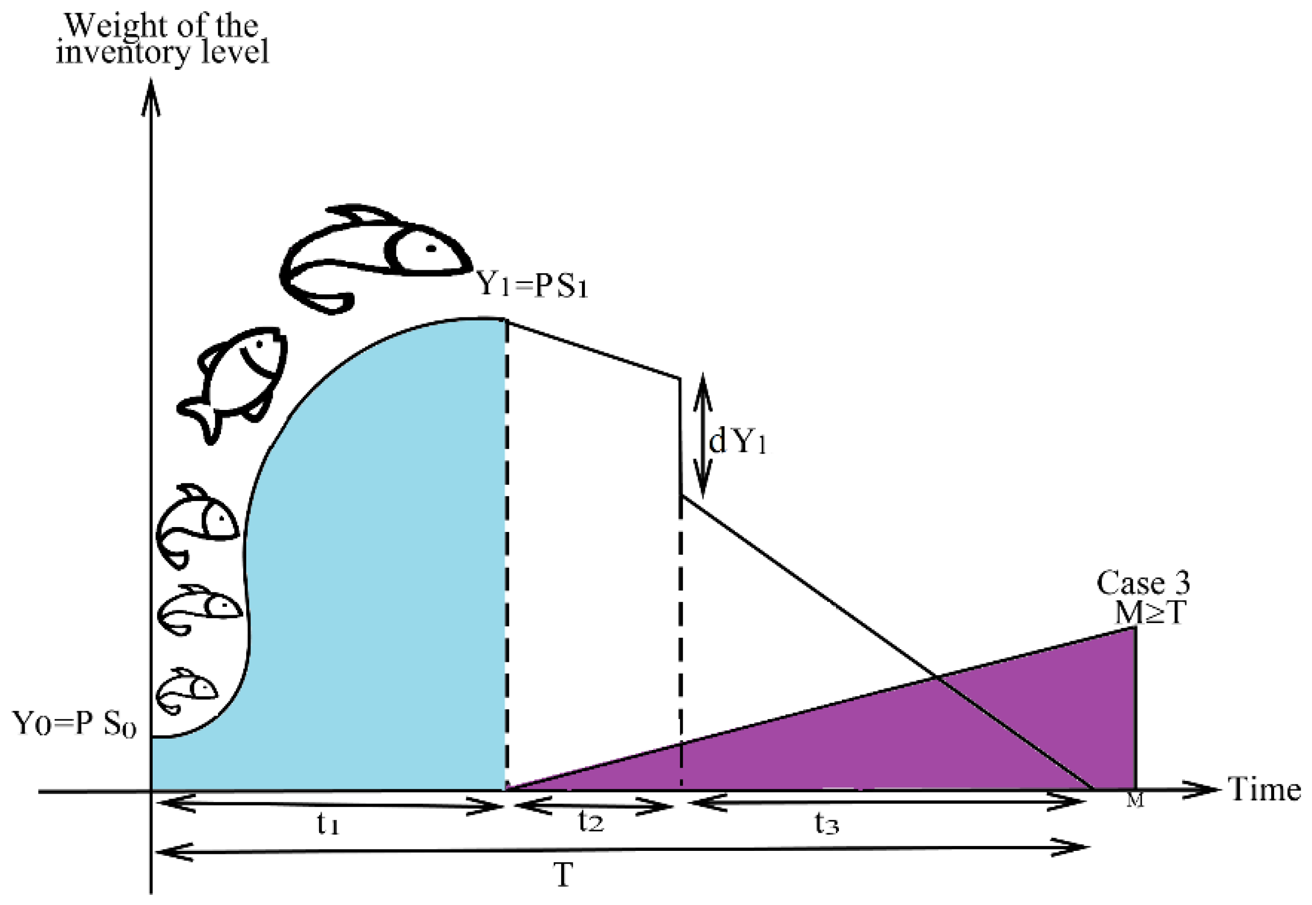
3.2. Model Description

Suppose that the buyer orders newborn items, say $P$ at the staring of the growing cycle, and the newborn items have some weight $S_0$. Now the total weight of inventory is $Y_0=P{S}_0$ and it is also considered that after time $t_1$ its weight is $S_1$ then the whole weight of the inventory as $Y_1=P{S}_1$. After the whole lot is received, the buyer inspects the whole lot during the time period ${\mathit{t}}_{\mathbf{2}}$ with the screening rate $R$ and divides the whole lot into two categories: one is the good quality items and the other is the defective quality items. It is assumed the percentage of defective items in the whole lot is $d\left(n\right)$ and the whole defective items are $d\left(n\right){\mathit{Y}}_{\mathbf{1}}$ while the non-defective items are $(1-d\left(n\right)){\mathit{Y}}_{\mathbf{1}}$. The buyer sales the defective items at low prices during the time period ${\mathit{t}}_{\mathbf{3}}$ and the good quality at a high price. The carrying costs are included for the time period of consumption time, and we have described it in Figure 4 briefly. The accepted policy of trade credit is also described in Figure 5. We included some costs such as purchasing cost $\left(PC=P_{c}P{S}_0\right)$, ordering cost $\left(OC=K\right)$, inventory carrying cost $(IHC=h\left(\frac{P^2{\left(1-d \left(n\right)\right)}^2}{2D}+\frac{P^2{S}_1^{2}d\left(n\right)}{R}\right)$, inspection cost $\left(IC=I_s{Y}_1\right)$, carbon emission cost $\left(CEC=2 d_1{E}_t{T}_{ci}\right)$ due to carbon units exit during transportation and feeding cost $\left(FC\right)$. The buyer obtains the whole revenue $\left(TR=S_{g}P{S}_1\left(1-d\left(n\right)\right)+S_{d}P{S}_{1}d\left(n\right)\right)$ from the other sources. The whole profit is given below:

The whole buyer’s profit

$$\xi \left(P\right)=\mathrm{whole} \mathrm{sales} \mathrm{revenue}\left(TR\right)-\mathrm{whole} \mathrm{inventory} \mathrm{cost}\left(TC\right)$$

$$\xi \left(P\right)=\left(S_{g}P{S}_1\left(1-d\left(n\right)\right)+S_{d}P{S}_{1}d\left(n\right) \right)-\left(P_{c}P{S}_0+K+h\left(\frac{P^2{\left(1-d \left(n\right)\right)}^2}{2D}+\frac{P^2{S}_1^{2}d\left(n\right)}{R}\right)+I_{s}P{S}_1{}_{ }+2 d_{1}e{T}_{ci}+FC\right)$$

(3)

In Equation (3), the feeding cost (FC) can be calculated with the help of the growth linear function ($S_t$), which gives

$$FC=f_{d}P{{\displaystyle \int }}_0^{t_1}{S}_{t}dt$$

(4)

From Equation (4), the value of feeding cost (FC) putting in Equation (3), and we obtain

$$\xi \left(P\right)=\left(S_{g}P{S}_1\left(1-d\left(n\right)\right)+S_{d}P{S}_{1}d\left(n\right) \right)-\left(P_{c}P{S}_0+K+h\left(\frac{P^2{\left(1-d \left(n\right)\right)}^2}{2D}+\frac{P^2{S}_1^{2}d\left(n\right)}{R}\right)+I_{s}P{S}_1{}_{ }+2 d_{1}e{T}_{ci}+f_{d}P{{\displaystyle \int }}_0^{t_1}{S}_{t}dt\right)$$

(5)

For the calculation of the buyer’s whole profit, the feeding function is needed for the growing items, and its value is different for different items. To calculate the feeding cost, the growth function is needed. Here, we discuss the logistic growth functions for the calculation of feeding costs. The logistic growth function is one type of growth function that relates the weight of the items with time and has three parameters; one is the weight under an asymptotic situation $\left(B\right)$, the second is the constant of integration $\left(l\right)$, and the third is the exponentially growth rate $\left(\mu \right)$. The growth function of the growing items is defined and briefly given in Sebatjane and Adetunji [13].

From Figure 4, the weight of an item rises slowly in the initial stage and steadily rises over time, up to the maturity level; after that, the weight gain reduces. At the initial stage, the stock of the inventory is $Y_0\left(=P{S}_0\right).$ The inventory level at the maturity time $t_1$ is $Y_1\left(=P{S}_1\right)$. The whole items screened up to time $t_2$.

$$S_t=\frac{B}{1+l{e}^{-\mu t}}$$

(6)

From Equation (6), we can calculate for $t_1$ and we obtain

$$t_1=-\frac{\log \left(\frac{B}{l{S}_1}-\frac{1}{l}\right) }{\mu }$$

(7)

Hence, the feeding cost (FC) can be calculated from Figure 3, and we obtain

$$FC=f_{d}P{{\displaystyle \int }}_0^{t_1}{S}_{t}dt=f_{d}P{{\displaystyle \int }}_0^{\frac{-\log \left(\frac{B}{l{S}_1}-\frac{1}{l}\right) }{\mu }}\frac{B}{1+l{e}^{-\mu t}} dt$$

$$FC=f_{d}P{{\displaystyle \int }}_0^{\frac{-\log \left(\frac{B}{l{S}_1}-\frac{1}{l}\right) }{\mu }}\frac{B}{1+l{e}^{-\mu t}} dt$$

$$FC=f_{d}P\left({\mathrm{B} \mathrm{t}}_1+\frac{\mathrm{B}}{\mu }\log \left(\frac{1+l{e}^{-\mu t}}{1+l}\right)\right)$$

(8)

The buyer’s whole profit under the logistic growth function from Equation (5) and Equation (8); we obtain

$${\xi }_{LGF}\left(P\right)=\left(S_{g}P{S}_1\left(1-d\left(n\right)\right)+S_{d}P{S}_{1}d\left(n\right) \right)-(P_{c}P{S}_0+K+h\left(\frac{P^2{\left(1-d \left(n\right)\right)}^2}{2D}+\frac{P^2{S}_1^{2}d\left(n\right)}{R}\right)+I_{s}P{S}_1{}_{ }+2 d_1{E}_t{T}_{ci}+f_{d}P\left({\mathrm{B} \mathrm{t}}_1+\frac{\mathrm{B}}{\mu }\log \left(\frac{1+l{e}^{-\mu t}}{1+l}\right)\right))$$

(9)

The seller offers the credit financing period to the buyer, and the buyer accepts the scheme of the trade credit policy. The buyer’s total profit under the trade credit scheme is given in Equation (10) below:

$$\xi \left(P\right)=(S_{g}P{S}_1\left(1-d\left(n\right)\right)+S_{d}P{S}_{1}d\left(n\right) +\mathrm{IE})-(P_{c}P{S}_0+K+h\left(\frac{P^2{\left(1-d \left(n\right)\right)}^2}{2D}+\frac{P^2{S}_1^{2}d\left(n\right)}{R}\right)+I_{s}P{S}_1{}_{ }+2 d_1{E}_t{T}_{ci}+f_{d}P\left({\mathrm{B} \mathrm{t}}_1+\frac{\mathrm{B}}{\mu }\log \left(\frac{1+l{e}^{-\mu t}}{1+l}\right)\right)+IP)$$

(10)

From Equation (10), the values of interest gained (IE) and interest charged (IP) depend on some situations of credit period, which are (i) $0\le M\le t_2$ (ii) $M\le t_2\le T$ (iii) $T\le M$ and explained briefly in Figure 5.

Case-1:

$0\le M\le t_2$

From Figure 6, the buyer obtains interest gained in the credit period from $0$ to $M$ and revenue earned on the sale of items. The interest gained (IE) for the buyer is calculated and equal $D{\left(M-t_1\right)}^2{I}_e{S}_g/2$. The interest paid (IP) for the buyer is calculated from the time period $M$ to $T$ and due to the unsold items, which is equal to $\frac{D{\left(T-M\right)}^2{I}_p{P}_c}{2}+Pd\left(n\right)\left(t_2-M-t_1\right)I_p{P}_c$.

Now, the buyer’s total profit in this scenario is

$${\xi }_1\left(P\right)=(S_{g}P{S}_1\left(1-d\left(n\right)\right)+S_{d}P{S}_{1}d\left(n\right) +D{\left(M-t_1\right)}^2{I}_e{S}_g/2)-(P_{c}P{S}_0+K+h\left(\frac{P^2{\left(1-d \left(n\right)\right)}^2}{2D}+\frac{P^2{S}_1^{2}d\left(n\right)}{R}\right)+I_{s}P{S}_1{}_{ }+2 d_1{E}_t{T}_{ci}+f_{d}P\left({\mathrm{B} \mathrm{t}}_1+\frac{\mathrm{B}}{\mu }\log \left(\frac{1+l{e}^{-\mu t}}{1+l}\right)\right)+\frac{D{\left(T-M\right)}^2{I}_p{P}_c}{2}+Pd\left(n\right)\left(t_M-M-t_1\right)I_p{P}_c)$$

(11)

Case-2:

$t_2\le M\le T$

In this case, from Figure 6, the buyer earns interest gained and revenue for the sold items, which are equal to $\frac{D{\left(M-t_1\right)}^2{I}_e{S}_g}{2}+Pd\left(n\right)\left(M-t_2-t_1\right)I_e{S}_d$ and the buyer pays interest for unsold items, which is equal to $\frac{D{\left(T-M\right)}^2{I}_p{P}_c}{2}$.

Now, the buyer’s total profit in this scenario is

$$\begin{gathered} {\xi }_2\left(P\right)=(S_{g}P{S}_1\left(1-d\left(n\right)\right)+S_{d}P{S}_{1}d\left(n\right) +\frac{D{\left(M-t_1\right)}^2{I}_e{S}_g}{2}+Pd\left(n\right)\left(M-t_2-t_1\right)I_e{S}_d) \\ -(P_{c}P{S}_0+K+h\left(\frac{P^2{\left(1-d \left(n\right)\right)}^2}{2D}+\frac{P^2{S}_1^{2}d\left(n\right)}{R}\right)+I_{s}P{S}_1{}_{ }+2 d_1{E}_t{T}_{ci} \\ +f_{d}P\left({\mathrm{B} \mathrm{t}}_1+\frac{\mathrm{B}}{\mu }\log \left(\frac{1+l{e}^{-\mu t}}{1+l}\right)\right)+\frac{D{\left(T-M\right)}^2{I}_p{P}_c}{2}) \end{gathered}$$

(12)

Case-3:

$t_2\le T\le M$

The buyer obtains interest gained from the whole up to the time period T and its value is $\frac{D{\left(T\right)}^2{I}_e{S}_g}{2}+Pd\left(n\right)\left(M-t_2-t_1\right)I_e{S}_d+\left(M-T\right)DT{I}_e{S}_g$, and the buyer does not give any interest paid, which is equal to zero.

Now, the buyer’s total profit in this scenario is

$${\xi }_3\left(P\right)=(S_{g}P{S}_1\left(1-d\left(n\right)\right)+S_{d}P{S}_{1}d\left(n\right) +\frac{D{\left(T\right)}^2{I}_e{S}_g}{2}+Pd\left(n\right)\left(M-t_2-t_1\right)I_e{S}_d+\left(M-T\right)DT{I}_e{S}_g)-(P_{c}P{S}_0+K+h\left(\frac{P^2{\left(1-d \left(n\right)\right)}^2}{2D}+\frac{P^2{S}_1^{2}d\left(n\right)}{R}\right)+I_{s}P{S}_1{}_{ }+2 d_1{E}_t{T}_{ci}+f_{d}P\left({\mathrm{B} \mathrm{t}}_1+\frac{\mathrm{B}}{\mu }\log \left(\frac{1+l{e}^{-\mu t}}{1+l}\right)\right))$$

(13)

In this order, we are moving in the direction of the fuzzy concept and also have discussed the fuzzify and defuzzify of the buyer’s total profit for each case in the forthcoming section.

4. Proposed Model under Fuzzy Environment

In real-world transactions, considering the unstable environment, it would not be easy to calculate the exact value of the inventory parameters. Therefore, the decision-makers calculate the approximate value of these parameters. The triangular fuzzy number represents the uncertainty. In this model, the triangular fuzzy number is used to fuzzify the buyer’s total profit for each case, and after that, the signed distance method is applied to defuzzify the buyer’s total fuzzy profit for each case. From the assumption, we considered that the demand rate is imprecise in nature and taken as a triangular fuzzy number, $\tilde{D}=\left(D-{\mathsf{\Delta }}_l,D,D+{\mathsf{\Delta }}_h\right)$ and the total profit of each case is defuzzified with the help of the signed distance method.

The buyer’s total profit under case 1 is reduced into a total fuzzy profit from Equation (11)

$${\tilde{\xi }}_1\left(P\right)=(S_{g}P{S}_1\left(1-d\left(n\right)\right)+S_{d}P{S}_{1}d\left(n\right) +\tilde{D}{\left(M-t_1\right)}^2{I}_e{S}_g/2)-(P_{c}P{S}_0+K+h\left(\frac{P^2{\left(1-d \left(n\right)\right)}^2}{2\tilde{D}}+\frac{P^2{S}_1^{2}d\left(n\right)}{R}\right)+I_{s}P{S}_1{}_{ }+2 d_1{E}_t{T}_{ci}+f_{d}P\left({\mathrm{B} \mathrm{t}}_1+\frac{\mathrm{B}}{\mu }\log \left(\frac{1+l{e}^{-\mu t}}{1+l}\right)\right)+\frac{\tilde{D}{\left(T-M\right)}^2{I}_p{P}_c}{2}+Pd\left(n\right)\left(t_M-M-t_1\right)I_p{P}_c)$$

(14)

From Equation (14), we defuzzified the buyer’s total fuzzy profit under case 1, and we obtain

$${\tilde{\xi }}_1(P)={\xi }_{11}(P)=d\left({\tilde{\xi }}_1\right(P),0)=(S_{g}P{S}_1\left(1-d\left(n\right)\right)+S_{d}P{S}_{1}d\left(n\right) +d(\tilde{D},\tilde{0}){\left(M-t_1\right)}^2{I}_e{S}_g/2)-(P_{c}P{S}_0+K+h\left(\frac{P^2{\left(1-d \left(n\right)\right)}^2}{2d(\tilde{D},\tilde{0})}+\frac{P^2{S}_1^{2}d\left(n\right)}{R}\right)+I_{s}P{S}_1{}_{ }+2 d_1{E}_t{T}_{ci}+f_{d}P\left({\mathrm{B} \mathrm{t}}_1+\frac{\mathrm{B}}{\mu }\log \left(\frac{1+l{e}^{-\mu t}}{1+l}\right)\right)+\frac{d(\tilde{D},\tilde{0}){\left(T-M\right)}^2{I}_p{P}_c}{2}+Pd\left(n\right)\left(t_M-M-t_1\right)I_p{P}_c)$$

(15)

Now, using the definition of the signed distance method from Equation (2) in Equation (15), we obtain

$${\xi }_{11}(P)=d\left({\tilde{\xi }}_1\right(P),0)=(S_{g}P{S}_1\left(1-d\left(n\right)\right)+S_{d}P{S}_{1}d\left(n\right) +\left(\frac{4D+{\mathsf{\Delta }}_h-{\mathsf{\Delta }}_l}{4}\right){\left(M-t_1\right)}^2{I}_e{S}_g/2)-(P_{c}P{S}_0+K+h\left(\frac{P^2{\left(1-d \left(n\right)\right)}^2}{2\left(\frac{4D+{\mathsf{\Delta }}_h-{\mathsf{\Delta }}_l}{4}\right)}+\frac{P^2{S}_1^{2}d\left(n\right)}{R}\right)+I_{s}P{S}_1{}_{ }+2 d_1{E}_t{T}_{ci}+f_{d}P\left({\mathrm{B} \mathrm{t}}_1+\frac{\mathrm{B}}{\mu }\log \left(\frac{1+l{e}^{-\mu t}}{1+l}\right)\right)+\frac{\left(\frac{4D+{\mathsf{\Delta }}_h-{\mathsf{\Delta }}_l}{4}\right){\left(T-M\right)}^2{I}_p{P}_c}{2}+Pd\left(n\right)\left(t_M-M-t_1\right)I_p{P}_c)$$

(16)

Now, the buyer’s total fuzzy profit per cycle for the case 1 using Equation (16)

$${\xi }_{111}\left(P\right)=\frac{1}{T}\left({\xi }_{11}\left(P\right)\right) \mathrm{where} T=\frac{P{S}_1\left(1-d\left(n\right)\right)}{\left(\frac{4D+{\mathsf{\Delta }}_h-{\mathsf{\Delta }}_l}{4}\right)}$$

$${\xi }_{111}(P)=\frac{\left(\frac{4D+{\mathsf{\Delta }}_h-{\mathsf{\Delta }}_l}{4}\right)}{P{S}_1\left(1-d\left(n\right)\right)}((S_{g}P{S}_1\left(1-d\left(n\right)\right)+S_{d}P{S}_{1}d\left(n\right) +\left(\frac{4D+{\mathsf{\Delta }}_h-{\mathsf{\Delta }}_l}{4}\right){\left(M-t_1\right)}^2{I}_e{S}_g/2)-(P_{c}P{S}_0+K+h\left(\frac{P^2{\left(1-d \left(n\right)\right)}^2}{2\left(\frac{4D+{\mathsf{\Delta }}_h-{\mathsf{\Delta }}_l}{4}\right)}+\frac{P^2{S}_1^{2}d\left(n\right)}{R}\right)+I_{s}P{S}_1{}_{ }+2 d_1{E}_t{T}_{ci}+f_{d}P\left({\mathrm{B} \mathrm{t}}_1+\frac{\mathrm{B}}{\mu }\log \left(\frac{1+l{e}^{-\mu t}}{1+l}\right)\right)+\frac{\left(\frac{4D+{\mathsf{\Delta }}_h-{\mathsf{\Delta }}_l}{4}\right){\left(T-M\right)}^2{I}_p{P}_c}{2}+Pd\left(n\right)\left(t_M-M-t_1\right)I_p{P}_c)$$

(17)

The buyer’s total profit under case 2 is reduced into a total fuzzy profit from Equation (12)

$${\xi }_2\left(P\right)=(S_{g}P{S}_1\left(1-d\left(n\right)\right)+S_{d}P{S}_{1}d\left(n\right) +\frac{\tilde{D}{\left(M-t_1\right)}^2{I}_e{S}_g}{2}+Pd\left(n\right)\left(M-t_2-t_1\right)I_e{S}_d)-(P_{c}P{S}_0+K+h\left(\frac{P^2{\left(1-d \left(n\right)\right)}^2}{2\tilde{D}}+\frac{P^2{S}_1^{2}d\left(n\right)}{R}\right)+I_{s}P{S}_1{}_{ }+2 d_1{E}_t{T}_{ci}+f_{d}P\left({\mathrm{B} \mathrm{t}}_1+\frac{\mathrm{B}}{\mu }\log \left(\frac{1+l{e}^{-\mu t}}{1+l}\right)\right)+\frac{\tilde{D}{\left(T-M\right)}^2{I}_p{P}_c}{2})$$

(18)

From Equation (18), we defuzzified the buyer’s total fuzzy profit under case 2, and we obtain

$${\tilde{\xi }}_2(P)={\xi }_{22}(P)=d\left({\tilde{\xi }}_2\right(P),0)=(S_{g}P{S}_1\left(1-d\left(n\right)\right)+S_{d}P{S}_{1}d\left(n\right) +\frac{d(\tilde{D},\tilde{0}){\left(M-t_1\right)}^2{I}_e{S}_g}{2}+Pd\left(n\right)\left(M-t_2-t_1\right)I_e{S}_d)-(P_{c}P{S}_0+K+h\left(\frac{P^2{\left(1-d \left(n\right)\right)}^2}{2d(\tilde{D},\tilde{0})}+\frac{P^2{S}_1^{2}d\left(n\right)}{R}\right)+I_{s}P{S}_1{}_{ }+2 d_1{E}_t{T}_{ci}+f_{d}P\left({\mathrm{B} \mathrm{t}}_1+\frac{\mathrm{B}}{\mu }\log \left(\frac{1+l{e}^{-\mu t}}{1+l}\right)\right)+\frac{d(\tilde{D},\tilde{0}){\left(T-M\right)}^2{I}_p{P}_c}{2})$$

(19)

Now, using the definition of the signed distance method from Equation (2) in Equation (19), we obtain

$${\xi }_{22}(P)=d\left({\tilde{\xi }}_2\right(P),0)=(S_{g}P{S}_1\left(1-d\left(n\right)\right)+S_{d}P{S}_{1}d\left(n\right) +\frac{\left(\frac{4D+{\mathsf{\Delta }}_h-{\mathsf{\Delta }}_l}{4}\right){\left(M-t_1\right)}^2{I}_e{S}_g}{2}+Pd\left(n\right)\left(M-t_2-t_1\right)I_e{S}_d)-(P_{c}P{S}_0+K+h\left(\frac{P^2{\left(1-d \left(n\right)\right)}^2}{2\left(\frac{4D+{\mathsf{\Delta }}_h-{\mathsf{\Delta }}_l}{4}\right)}+\frac{P^2{S}_1^{2}d\left(n\right)}{R}\right)+I_{s}P{S}_1{}_{ }+2 d_1{E}_t{T}_{ci}+f_{d}P\left({\mathrm{B} \mathrm{t}}_1+\frac{\mathrm{B}}{\mu }\log \left(\frac{1+l{e}^{-\mu t}}{1+l}\right)\right)+\frac{\left(\frac{4D+{\mathsf{\Delta }}_h-{\mathsf{\Delta }}_l}{4}\right){\left(T-M\right)}^2{I}_p{P}_c}{2})$$

(20)

Now, the buyer’s total fuzzy profit per cycle for the case 2 using Equation (20)

$${\xi }_{222}\left(P\right)=\frac{1}{T}\left({\xi }_{22}\left(P\right)\right) \mathrm{where} T=\frac{P{S}_1\left(1-d\left(n\right)\right)}{\left(\frac{4D+{\mathsf{\Delta }}_h-{\mathsf{\Delta }}_l}{4}\right)}$$

$${\xi }_{222}(P)=\frac{\left(\frac{4D+{\mathsf{\Delta }}_h-{\mathsf{\Delta }}_l}{4}\right)}{P{S}_1\left(1-d\left(n\right)\right)}=\left(\right(S_{g}P{S}_1\left(1-d\left(n\right)\right)+S_{d}P{S}_{1}d\left(n\right) +\frac{\left(\frac{4D+{\mathsf{\Delta }}_h-{\mathsf{\Delta }}_l}{4}\right){\left(M-t_1\right)}^2{I}_e{S}_g}{2}+Pd\left(n\right)\left(M-t_2-t_1\right)I_e{S}_d)-(P_{c}P{S}_0+K+h\left(\frac{P^2{\left(1-d \left(n\right)\right)}^2}{2\left(\frac{4D+{\mathsf{\Delta }}_h-{\mathsf{\Delta }}_l}{4}\right)}+\frac{P^2{S}_1^{2}d\left(n\right)}{R}\right)+I_{s}P{S}_1{}_{ }+2 d_1{E}_t{T}_{ci}+f_{d}P\left({\mathrm{B} \mathrm{t}}_1+\frac{\mathrm{B}}{\mu }\log \left(\frac{1+l{e}^{-\mu t}}{1+l}\right)\right)+\frac{\left(\frac{4D+{\mathsf{\Delta }}_h-{\mathsf{\Delta }}_l}{4}\right){\left(T-M\right)}^2{I}_p{P}_c}{2}\left)\right)$$

(21)

The buyer’s total profit under case 3 is reduced into a total fuzzy profit from Equation (13)

$${\tilde{\xi }}_3\left(P\right)=(S_{g}P{S}_1\left(1-d\left(n\right)\right)+S_{d}P{S}_{1}d\left(n\right) +\tilde{D}\frac{{\left(T\right)}^2{I}_e{S}_g}{2}+Pd\left(n\right)\left(M-t_2-t_1\right)I_e{S}_d+(M-T)\tilde{D}T{I}_e{S}_d)-(P_{c}P{S}_0+K+h\left(\frac{P^2{\left(1-d \left(n\right)\right)}^2}{2\tilde{D}}+\frac{P^2{S}_1^{2}d\left(n\right)}{R}\right)+I_{s}P{S}_1{}_{ }+2 d_1{E}_t{T}_{ci}+f_{d}P\left({\mathrm{B} \mathrm{t}}_1+\frac{\mathrm{B}}{\mu }\log \left(\frac{1+l{e}^{-\mu t}}{1+l}\right)\right))$$

(22)

From Equation (22), we defuzzified the buyer’s total fuzzy profit under case 3, and we obtain

$${\tilde{\xi }}_3\left(P\right)={\xi }_{33}\left(P\right)=d({\tilde{\xi }}_3(P),\tilde{0})=(S_{g}P{S}_1\left(1-d\left(n\right)\right)+S_{d}P{S}_{1}d\left(n\right) +d(\tilde{D},\tilde{0})\frac{{\left(T\right)}^2{I}_e{S}_g}{2}+Pd\left(n\right)(M-t_2-t_1)I_e{S}_d+(M-Td(\tilde{D},\tilde{0}))T{I}_e{S}_g)-(P_{c}P{S}_0+K+h\left(\frac{P^2{\left(1-d \left(n\right)\right)}^2}{2d(\tilde{D},\tilde{0})}+\frac{P^2{S}_1^{2}d\left(n\right)}{R}\right)+I_{s}P{S}_1{}_{ }+2 d_1{E}_t{T}_{ci}+f_{d}P\left({\mathrm{B} \mathrm{t}}_1+\frac{\mathrm{B}}{\mu }\log \left(\frac{1+l{e}^{-\mu t}}{1+l}\right)\right))$$

(23)

Now, using the definition of the signed distance method from Equation (2) in Equation (23), we obtain

$${\xi }_{33}\left(P\right)=d({\tilde{\xi }}_3(P),\tilde{0})=(S_{g}P{S}_1\left(1-d\left(n\right)\right)+S_{d}P{S}_{1}d\left(n\right) +\left(\frac{4D+{\mathsf{\Delta }}_h-{\mathsf{\Delta }}_l}{4}\right)\frac{{\left(T\right)}^2{I}_e{S}_g}{2}+Pd\left(n\right)(M-t_2-t_1)I_e{S}_d+(M-T)(\frac{4D+{\mathsf{\Delta }}_h-{\mathsf{\Delta }}_l}{4})T{I}_e{S}_g)-(P_{c}P{S}_0+K+h\left(\frac{P^2{\left(1-d \left(n\right)\right)}^2}{2\left(\frac{4D+{\mathsf{\Delta }}_h-{\mathsf{\Delta }}_l}{4}\right)}+\frac{P^2{S}_1^{2}d\left(n\right)}{R}\right)+I_{s}P{S}_1{}_{ }+2 d_1{E}_t{T}_{ci}+f_{d}P\left({\mathrm{B} \mathrm{t}}_1+\frac{\mathrm{B}}{\mu }\log \left(\frac{1+l{e}^{-\mu t}}{1+l}\right)\right))$$

(24)

Now, the buyer’s total fuzzy profit per cycle for case 3 using Equation (24):

$${\xi }_{333}\left(P\right)=\frac{1}{T}\left({\xi }_{33}\left(P\right)\right) \mathrm{where} T=\frac{P{S}_1\left(1-d\left(n\right)\right)}{\left(\frac{4D+{\mathsf{\Delta }}_h-{\mathsf{\Delta }}_l}{4}\right)}$$

$${\xi }_{333}(P)=\frac{\left(\frac{4D+{\mathsf{\Delta }}_h-{\mathsf{\Delta }}_l}{4}\right)}{P{S}_1\left(1-d\left(n\right)\right)}=\left(\right(S_{g}P{S}_1\left(1-d\left(n\right)\right)+S_{d}P{S}_{1}d\left(n\right) +\left(\frac{4D+{\mathsf{\Delta }}_h-{\mathsf{\Delta }}_l}{4}\right)\frac{{\left(T\right)}^2{I}_e{S}_g}{2}+Pd\left(n\right)\left(M-t_2-t_1\right)I_e{S}_d+(M-T)(\frac{4D+{\mathsf{\Delta }}_h-{\mathsf{\Delta }}_l}{4})T{I}_e{S}_g)-(P_{c}P{S}_0+K+h\left(\frac{P^2{\left(1-d \left(n\right)\right)}^2}{2\left(\frac{4D+{\mathsf{\Delta }}_h-{\mathsf{\Delta }}_l}{4}\right)}+\frac{P^2{S}_1^{2}d\left(n\right)}{R}\right)+I_{s}P{S}_1{}_{ }+2 d_1{E}_t{T}_{ci}+f_{d}P\left({\mathrm{B} \mathrm{t}}_1+\frac{\mathrm{B}}{\mu }\log \left(\frac{1+l{e}^{-\mu t}}{1+l}\right)\right)\left)\right)$$

(25)

5. Solution Method

The solution methodology has been taken from Mittal and Sharma [24] for case 1, case 2, and case 3. The decision variable $\left(P\right)$ has been calculated with the help of the maxima minima test, and the necessary conditions for finding the decision variable are $\frac{d\left(\xi \left(P\right)\right)}{dP}=0$. After that, we calculated the value of the decision variable, and the value of the decision variable is optimal if it satisfies the sufficient condition $\frac{d^2\left(\xi \left(P\right)\right)}{d{P}^2}\le 0$ at $P$, which also represents the concavity of the buyer’s total fuzzy profit with respect to the optimal value of the decision variable, then the value of the decision variable $\left(P\right)$ can be termed as optimal and it is represented by $\left(P^{\ast }\right)$. The optimal value of the decision variable maximizes the buyer’s total fuzzy profit.

5.1. Solution Method for Case 1

From Equation (17), we can write for the optimal value of $P,$

$$\frac{d\left({\xi }_{111}\left(P\right)\right)}{dP}=0$$

(26)

After solving Equation (26) and the calculation has been given in Appendix A part ((A1)–(A3)), we obtain the value of $P$:

$$P=\sqrt{\frac{2RK\left(\frac{4D+{\mathsf{\Delta }}_h-{\mathsf{\Delta }}_l}{4}\right)-{\left(\frac{4D+{\mathsf{\Delta }}_h-{\mathsf{\Delta }}_l}{4}\right)}^2{(M-t_1)}^2{I}_e{S}_g+{\left(\frac{4D+{\mathsf{\Delta }}_h-{\mathsf{\Delta }}_l}{4}\right)}^2{M}^2{I}_p{P}_c}{2\left(\frac{4D+{\mathsf{\Delta }}_h-{\mathsf{\Delta }}_l}{4}\right)I_{p}d{\left(n\right)}_{ }{P}_c{S}_1+S_1^{2}Rh{\left(1-d\left(n\right)\right)}^2+2\left(\frac{4D+{\mathsf{\Delta }}_h-{\mathsf{\Delta }}_l}{4}\right) h{S}_1^{2}d\left(n\right)+R{I}_p{P}_c{S}_1^2{\left(1-d\left(n\right)\right)}^2} }$$

(27)

The value of $P$, from Equation (27) and putting in Equation (28), we obtain

$$\frac{d^2\left({\xi }_{111}\left(P\right)\right)}{d{P}^2}=\frac{-2K\left(\frac{4D+{\mathsf{\Delta }}_h-{\mathsf{\Delta }}_l}{4}\right)}{P^3{S}_1(1-d\left(n\right))}-\frac{{\left(\frac{4D+{\mathsf{\Delta }}_h-{\mathsf{\Delta }}_l}{4}\right)}^{2}P{I}_p{M}^2}{(1-d\left(n\right))P^3{S}_1}+\frac{S_g{I}_e{\left(\frac{4D+{\mathsf{\Delta }}_h-{\mathsf{\Delta }}_l}{4}\right)}^2{(M-t_1)}^2}{(1-d\left(n\right))P^3{S}_1}<0$$

(28)

Now, we conclude that the value of $P$ from Equation (26) is optimal because it satisfies Equation (28), which represents the concavity of the total fuzzy profit for the case 1, and hence, we can write the optimal value of $P_1^{\ast }$,

$$P_1^{\ast }=\sqrt{\frac{2RK\left(\frac{4D+{\mathsf{\Delta }}_h-{\mathsf{\Delta }}_l}{4}\right)-{\left(\frac{4D+{\mathsf{\Delta }}_h-{\mathsf{\Delta }}_l}{4}\right)}^2{(M-t_1)}^2{I}_e{S}_g+{\left(\frac{4D+{\mathsf{\Delta }}_h-{\mathsf{\Delta }}_l}{4}\right)}^2{M}^2{I}_p{P}_c}{2\left(\frac{4D+{\mathsf{\Delta }}_h-{\mathsf{\Delta }}_l}{4}\right)I_{p}d{\left(n\right)}_{ }{P}_c{S}_1+S_1^{2}Rh{\left(1-d\left(n\right)\right)}^2+2\left(\frac{4D+{\mathsf{\Delta }}_h-{\mathsf{\Delta }}_l}{4}\right) h{S}_1^{2}d\left(n\right)+R{I}_p{P}_c{S}_1^2{\left(1-d\left(n\right)\right)}^2} }$$

(29)

5.2. Solution Method for Case 2

From Equation (21), we can write for the optimal value of $P,$

$$\frac{d\left({\xi }_{222}\left(P\right)\right)}{dP}=0$$

(30)

We solved Equation (30), and the calculation has been given in Appendix A part ((A4)–(A6)); we obtain the value of $P$

$$P=\sqrt{\frac{2\left(\frac{4D+{\mathsf{\Delta }}_h-{\mathsf{\Delta }}_l}{4}\right)RK-{\left(\frac{4D+{\mathsf{\Delta }}_h-{\mathsf{\Delta }}_l}{4}\right)}^2{(M-t_1)}^2{I}_e{S}_{g}R+{\left(\frac{4D+{\mathsf{\Delta }}_h-{\mathsf{\Delta }}_l}{4}\right)}^2{M}^2{I}_p{P}_{c}R}{2\left(\frac{4D+{\mathsf{\Delta }}_h-{\mathsf{\Delta }}_l}{4}\right)d{\left(n\right)}_{ }{I}_e{P}_c{S}_1+S_1^{2}Rh{\left(1-d\left(n\right)\right)}^2+2h{S}_1^2\left(\frac{4D+{\mathsf{\Delta }}_h-{\mathsf{\Delta }}_l}{4}\right) d\left(n\right)+R{I}_p{P}_c{S}_1^2{\left(1-d\left(n\right)\right)}^2} }$$

(31)

Now, we find the second derivative of Equation (30), and putting the value of $P$ from Equation (31) in Equation (32) for the justification of the optimal value of $P$, we obtain

$$\frac{d^2\left({\xi }_{222}\left(P\right)\right)}{d{p}^2}=\frac{-2\left(\frac{4D+{\mathsf{\Delta }}_h-{\mathsf{\Delta }}_l}{4}\right)K}{\left(1-d\left(n\right)\right)P^3{S}_1}-\frac{P{I}_p{\left(\frac{4D+{\mathsf{\Delta }}_h-{\mathsf{\Delta }}_l}{4}\right)}^2{M}^2}{\left(1-d\left(n\right)\right)P^3{S}_1}+\frac{S_g{I}_e{\left(\frac{4D+{\mathsf{\Delta }}_h-{\mathsf{\Delta }}_l}{4}\right)}^2{\left(M-t_1\right)}^2}{\left(1-d\left(n\right)\right)P^3{S}_1}<0$$

(32)

From Equation (31), $P$ is the optimal value, and it is represented by $P_2^{\ast }$, and Equation (32) denotes the concavity of total fuzzy profit.

$$P_2^{\ast }=\sqrt{\frac{2\left(\frac{4D+{\mathsf{\Delta }}_h-{\mathsf{\Delta }}_l}{4}\right)RK-{\left(\frac{4D+{\mathsf{\Delta }}_h-{\mathsf{\Delta }}_l}{4}\right)}^2{(M-t_1)}^2{I}_e{S}_{g}R+{\left(\frac{4D+{\mathsf{\Delta }}_h-{\mathsf{\Delta }}_l}{4}\right)}^2{M}^2{I}_p{P}_{c}R}{2\left(\frac{4D+{\mathsf{\Delta }}_h-{\mathsf{\Delta }}_l}{4}\right)d{\left(n\right)}_{ }{I}_e{P}_c{S}_1+S_1^{2}Rh{\left(1-d\left(n\right)\right)}^2+2h{S}_1^2\left(\frac{4D+{\mathsf{\Delta }}_h-{\mathsf{\Delta }}_l}{4}\right) d\left(n\right)+R{I}_p{P}_c{S}_1^2{\left(1-d\left(n\right)\right)}^2} }$$

(33)

5.3. Solution Method for Case 3

From Equation (25), we can write for the optimal value of $P,$

$$\frac{d\left({\xi }_{333}\left(P\right)\right)}{dP}=0$$

(34)

We solved Equation (34), and the calculation has been given in Appendix A part ((A7)–(A9)); we obtain the value of $P$

$$P=\sqrt{\frac{2R\left(\frac{4D+{\mathsf{\Delta }}_h-{\mathsf{\Delta }}_l}{4}\right)K}{2D\left(\frac{4D+{\mathsf{\Delta }}_h-{\mathsf{\Delta }}_l}{4}\right)d{\left(n\right)}_{ }{I}_e{S}_d{S}_1+S_1^{2}Rh{\left(1-d\left(n\right)\right)}^2+2\left(\frac{4D+{\mathsf{\Delta }}_h-{\mathsf{\Delta }}_l}{4}\right) h{S}_1^{2}d\left(n\right)+r{I}_p{S}_g{S}_1^2{\left(1-d\left(n\right)\right)}^2} }$$

(35)

Now, we find the second derivative of Equation (34), and putting the value of $P$ from Equation (35) in Equation (36) for the justification of the optimal value of $P$, we obtain

$$\frac{d^2\left({\xi }_{333}\left(P\right)\right)}{d{p}^2}=\frac{-4RK{\left(\frac{4D+{\mathsf{\Delta }}_h-{\mathsf{\Delta }}_l}{4}\right)}_{ }}{p^3}<0.$$

(36)

From Equation (34), $P$ is the optimal value, and it is represented by $P_3^{\ast }$, and Equation (36) denotes the concavity of total fuzzy profit.

$$P_3^{\ast }=\sqrt{\frac{2R\frac{4D+{\mathsf{\Delta }}_h-{\mathsf{\Delta }}_l}{4} K}{2D\frac{4D+{\mathsf{\Delta }}_h-{\mathsf{\Delta }}_l}{4} d{\left(n\right)}_{ }{I}_e{S}_d{S}_1+S_1^{2}Rh{\left(1-d\left(n\right)\right)}^2+2\frac{4D+{\mathsf{\Delta }}_h-{\mathsf{\Delta }}_l}{4} h{S}_{1}d\left(n\right)+r{I}_p{S}_g{S}_1^2{\left(1-d\left(n\right)\right)}^2} }$$

(37)

5.4. Algorithm

Jayaswal et al. [17] have followed the algorithm process:

Step 1: Replace all input parameters in Equations (29), (33), and (37) and calculate the value of $P_1^{\ast }$,$P_2^{\ast }$, and $P_3^{\ast }$.

Step 2: After the calculation of $P$, we find out the value of $t_2$ and $T$ along the Equations (29), (33), and (37) and compared with credit period $M$ in each case.

Step 3: If it satisfies the condition $0<M<t_2$ along Equation (29), then calculate the total fuzzy profit from Equation (17); otherwise, move to the next step.

Step 4: If it satisfies the condition $t_2<M<t_3$ along Equation (33), then calculate the total fuzzy profit from Equation (21); otherwise, move to the next step.

Step 5: If it satisfies the condition $t_2<T<M$ along Equation (37), then calculate the total fuzzy profit from Equation (25).

Step 6: In this case, we compare which case is better for this proposed model and use it for sensitivity analysis.

5.5. Numerical Example

We have adopted the inventory parameters (Sebatjane and Adetunji [13]) given in

Table 2. Recommended inventory parameters.

Inventory Parameter	Numerical Value of Inventory Parameter	Inventory Parameter	Numerical Value of Inventory Parameter
Fuzzy demand rate $\left(\tilde{D}\right)$	1,000,000 g/year	Holding cost $\left(h\right)$	0.04 ZAR/g/year
Upper deviation fuzzy demand rate $({\mathsf{\Delta }}_h)$	10,000 g/year	Ordering cost $\left(K\right)$	1000 ZAR/cycle
Lower deviation fuzzy demand rate $({\mathsf{\Delta }}_h)$	5000 g/year	Feeding cost $\left(f_d\right)$	0.2 ZAR/g/year
Weight of each newborn growing item $(S_0)$	57 g	Weight of each newborn growing item at slaughtering time $(S_1)$	1500 g
Purchasing cost $(P_c)$	0.025 ZAR/g	Selling price for good items $(S_g)$	0.05 ZAR/g
Inspection cost $\left(I_s\right)$	0.00025 ZAR/g	Selling price for defective items $(S_d)$	0.02 ZAR/g
Inspection rate $\left(R\right)$	5,256,000 g/year	Asymptotic weight $\left(B\right)$	6870 g
Constant of integration $\left(l\right)$	120	Growth rate $\left(\mu \right)$	40/year (0.11/day)
Carbon emissions per Km due to transport $\left(E_t\right)$	0.00077344	Distance covered in one way (Km) $\left(d_1\right)$	500 Km
Emissions tax rate $\left(T_{ci}\right)$	30 $ per Ton	Learning rate (b)	0.79
Learning supporting parameter $\left(a\right)$	40	Learning supporting parameter $\left(g\right)$	999
Number of shipments $\left(n\right)$	5	Interest earned $\left(I_e\right)$	0.05
Interest earned $\left(I_p\right)$	0.08	Trade credit period Interest earned $\left(M\right)$	0.363 year

.

Several learning curve models were fitted to the collected data, and the S-shaped logistic learning curve was found to fit well, and it is of the form $d\left(n\right)=\frac{a}{g+e^{bn}}$ where $a, g,$ and $b>0$ are model parameters, $n$ is the number of shipments.

First, test the condition to avoid shortages within the inspection period. The behavior of the inventory level is depicted in Figure 6, Figure 7 and Figure 8 to avoid shortages during the screening time $(t_2=\frac{Y_1}{R})$, the percentage of defective items is restricted to $\left(1-d\left(n\right)\right)Y_1\ge \tilde{D}{t}_2⟹\mathsf{\Delta }d\left(n\right)\le 1-\left(\frac{\tilde{D}}{R}\right)$ where $Y_1=P{S}_1$,$t_2=\frac{Y_1}{R}$ and $d\left(n\right)=\frac{a}{g+e^{bn}}$; otherwise, shortages will occur. We are discussing some contributions, such as Sebatjane and Adetunji [13], who calculated the optimal newborn items and the expected profit for the defective items under the Logistic growth function, which are 148 units and USD 34,641.73, respectively. There was no fuzzy learning theory in this model, but the inclusion of fuzzy learning theory has a positive effect. The maximum total fuzzy profit depends on the credit period, which has been discussed in the mathematical formulation. The effect of learning, credit policy, and fuzzy concept had a positive effect on the number of newborn items and the buyer’s total fuzzy profit. If, in this study, we had excluded the learning, credit policy, or fuzzy environment, then the optimal inventory of the number of newborn items would be $P^{\ast }=1890$ and the buyer’s total profit is ${\xi }^{\ast }\left(P^{\ast }\right)=\$1.03421\times {10}^8$. From step 6 of the algorithm, we obtain maximum fuzzy profit in case 3, and we have selected case 3 for the sensitivity analysis. The optimal number of newborn items per cycle is calculated in three different cases, and the maximum total fuzzy profit with the optimal number of newborn is discussed below in

Table 3. Optimal number of newborn items under different cases.

Cases $\mathit{M} \left(\mathbf{Year}\right), {\mathit{t}}_2 \left(\mathbf{Year}\right)$ $\mathbf{and} \mathit{T} \left(\mathbf{year}\right)$	Optimal Number of New Born Items	Buyer’s Total Fuzzy Profit
$\mathrm{Case} 1, 0<M<t_2$, $0<0.03<0.291$	$P_1^{\ast }=1023$	${\xi }_{111}^{\ast }\left(P_1^{\ast }\right)=\$1.05725\times {10}^8$
$\mathrm{Case} 2, t_2<M<t_3,0.328<0.342<0.35$	$P_2^{\ast }=1150$	${\xi }_{222}^{\ast }\left(P_2^{\ast }\right)=\$1.07725\times {10}^8$
$\mathrm{Case} 3, T<M, 0.007<0.363$	$P_3^{\ast }=1214$	${\xi }_{333}^{\ast }\left(P_3^{\ast }\right)=\$1.08725\times {10}^8$

. In Figure 7, the model presentation under the logistic growth function for the case $t_2\le M\le T$ is showcased below, and also underneath below Figure 8, describes the model presentation under logistic growth function for the case $t_2\le T\le M$.

6. Sensitivity Analysis

In this section, we discussed the impact of the number of shipments, the impact of learning, credit period, and lower and upper fuzzy deviation of the demand rate on the total fuzzy profit and presented from

Table 4. Impact of shipment on the fuzzy total profit.

$\mathbf{Number} \mathbf{of} \mathbf{Shipments} \left(\mathit{n}\right)$	$\mathbf{Number} \mathbf{of} \mathbf{New} \mathbf{Born} \mathbf{Items} \left({\mathit{P}}_3^{\ast }\right)$	$\mathbf{Fuzzy} \mathbf{Total} \mathbf{Profit} {\mathit{\xi }}_{333}^{\ast } \left({\mathit{P}}_3^{\ast }\right)$
1	1193	$\$1.08710\times {10}^8$
2	1194	$$1.08712\times {10}^8$
3	1197	$$1.08716\times {10}^8$
4	1203	$$1.08721\times {10}^8$
5	1214	$$1.08725\times {10}^8$

,

Table 5. Impact of credit period on the fuzzy total profit.

$\mathbf{Credit} \mathbf{Period} \left(\mathit{M}\right) \mathbf{year}$	$\mathbf{Number} \mathbf{of} \mathbf{New} \mathbf{Born} \mathbf{Items} \left({\mathit{P}}_3^{\ast }\right)$	$\mathbf{Total} \mathbf{Fuzzy} \mathbf{Profit} {\mathit{\xi }}_{333}^{\ast } \left({\mathit{P}}_3^{\ast }\right)$
0.1	1211	$$1.07475\times {10}^8$
0.2	1213	$$1.081\times {10}^8$
0.3	1214	$$1.08725\times {10}^8$

,

Table 6. Impact of learning rate on the total fuzzy profit.

$\mathbf{Learning} \mathbf{Rate} \left(\mathit{b}\right)$	$\mathbf{Number} \mathbf{of} \mathbf{New} \mathbf{Born} \mathbf{Items} \left({\mathit{P}}_3^{\ast }\right)$	$\mathbf{Total} \mathbf{Fuzzy} \mathbf{Profit} {\mathit{\xi }}_{333}^{\ast } \left({\mathit{P}}_3^{\ast }\right)$
0.3932	1195	$$1.08715\times {10}^8$
0.4932	1198	$$1.08719\times {10}^8$
0.5932	1201	$$1.08721\times {10}^8$
0.6932	1213	$$1.08724\times {10}^8$
0.7932	1214	$$1.08725\times {10}^8$
0.8932	1214	$$1.08725\times {10}^8$
0.9932	1214	$$1.08725\times {10}^8$

,

Table 7. Impact of lower and upper fuzzy deviation of fuzzy demand rate on the total fuzzy profit.

$$\begin{gathered} \mathbf{Upper} \mathbf{Deviation} \mathbf{of} \mathbf{Demand} \mathbf{Rate} \\ \left({\mathbf{\Delta }}_{\mathit{h}}\right) \end{gathered}$$	Fuzzy Demand Rate $\left(\tilde{\mathit{D}}\right)$	$\mathbf{Lower} \mathbf{Deviation} \mathbf{of} \mathbf{Demand} \mathbf{Rate} \left({\mathbf{\Delta }}_{\mathit{l}}\right)$	$\mathbf{Number} \mathbf{of} \mathbf{New} \mathbf{Born} \mathbf{Items} \left({\mathit{P}}_3^{\ast }\right)$	Total Fuzzy Profit ${\mathit{\xi }}_{333}^{\ast } \left({\mathit{P}}_3^{\ast }\right)$
4000 g/year	1,000,000 g/year	2000 g/year	1141	$$4.34679\times {10}^7$
6000 g/year	1,000,000 g/year	3000 g/year	1203	$$6.52202\times {10}^7$
8000 g/year	1,000,000 g/year	4000 g/year	1210	$$8.69729\times {10}^7$
10,000 g/year	1,000,000 g/year	5000 g/year	1214	$$1.08725\times {10}^8$

,

Table 8. Impact of feeding cost on the total fuzzy profit.

$\mathbf{Feeding} \mathbf{Cost} \left({\mathit{f}}_{\mathit{d}}\right) \mathbf{ZAR}/\mathbf{g}/\mathbf{Year}$	$\mathbf{Number} \mathbf{of} \mathbf{New} \mathbf{Born} \mathbf{Items} \left({\mathit{P}}_3^{\ast }\right)$	Total Fuzzy Profit ${\mathit{\xi }}_{333}^{\ast } \left({\mathit{P}}_3^{\ast }\right)$
0.2	1214	$$1.08725\times {10}^8$
0.3	1214	$$1.01635\times {10}^8$
0.4	1214	$

,

Table 9. Impact of holding cost on the total fuzzy profit.

$\mathbf{Holding} \mathbf{Cost} \left(\mathit{h}\right) \mathbf{ZAR}/\mathbf{g}/\mathbf{Year}$	$\mathbf{Number} \mathbf{of} \mathbf{New} \mathbf{Born} \mathbf{Items} \left({\mathit{P}}_3^{\ast }\right)$	Total Fuzzy Profit ${\mathit{\xi }}_{333}^{\ast } \left({\mathit{P}}_3^{\ast }\right)$
0.04	1214	$$1.08725\times {10}^8$
0.06	991	$$1.08084\times {10}^8$
0.08	858	$$1.07544\times {10}^8$

,

Table 10. Impact of inspection cost on the total fuzzy profit.

$\mathbf{Inspection} \mathbf{Cost} \left({\mathit{I}}_{\mathit{s}}\right) \mathbf{g}/\mathbf{Year}$	$\mathbf{Number} \mathbf{of} \mathbf{New} \mathbf{Born} \mathbf{Items} \left({\mathit{P}}_3^{\ast }\right)$	Total Fuzzy Profit ${\mathit{\xi }}_{333 }^{\ast }\left({\mathit{P}}_3^{\ast }\right)$
0.00025	1214	$$1.08725\times {10}^8$
0.00035	1214	$$1.08465\times {10}^8$
0.00045	1214	$$1.08205\times {10}^8$

,

Table 11. Impact of purchasing cost on the total fuzzy profit.

$\mathbf{Purchasing} \mathbf{Cost} \left({\mathit{P}}_{\mathit{c}}\right) \mathbf{ZAR}/\mathbf{g}$	$\mathbf{Number} \mathbf{of} \mathbf{New} \mathbf{Born} \mathbf{Items} \left({\mathit{P}}_3^{\ast }\right)$	Total Fuzzy Profit ${\mathit{\xi }}_{333}^{\ast } \left({\mathit{P}}_3^{\ast }\right)$
0.025	1214	$$1.08725\times {10}^8$
0.035	1214	$$1.07737\times {10}^8$
0.045	1214	$$1.06749\times {10}^8$

,

Table 12. Impact of selling cost on the total fuzzy profit.

$\mathbf{Selling} \mathbf{Price} ({\mathit{S}}_{\mathit{g}}) \mathbf{for} \mathbf{Good} \mathbf{Items}$	$\mathbf{Number} \mathbf{of} \mathbf{New} \mathbf{Born} \mathbf{Items} \left({\mathit{P}}_3^{\ast }\right)$	Total Fuzzy Profit ${\mathit{\xi }}_{333 }^{\ast }\left({\mathit{P}}_3^{\ast }\right)$
0.05	1214	$$1.08725\times {10}^8$
0.06	1214	$$1.341\times {10}^8$
0.07	1214	$$1.59474\times {10}^8$

,

Table 13. Impact of emissions tax rate $\left(T_{ci}\right)$ on the total fuzzy profit.

$\mathbf{Emissions} \mathbf{Tax} \mathbf{Rate} \left({\mathit{T}}_{\mathit{c}\mathit{i}}\right)$	$\mathbf{Number} \mathbf{of} \mathbf{New} \mathbf{Born} \mathbf{Items} \left({\mathit{P}}_3^{\ast }\right)$	Total Fuzzy Profit ${\mathit{\xi }}_{333}^{\ast } \left({\mathit{P}}_3^{\ast }\right)$
30 $	1214	$$1.08725\times {10}^8$
35 $	1214	$\$1.08719\times {10}^8$
40 $	1214	$$1.08712\times {10}^8$

and

Table 14. Impact of travel distance (one-way) on the total fuzzy profit.

$\mathbf{Emissions} \mathbf{Tax} \mathbf{Rate} \left({\mathit{T}}_{\mathit{c}\mathit{i}}\right)$	$\mathbf{Number} \mathbf{of} \mathbf{New} \mathbf{Born} \mathbf{Items} \left({\mathit{P}}_3^{\ast }\right)$	Total Fuzzy Profit ${\mathit{\xi }}_{333 }^{\ast }\left({\mathit{P}}_3^{\ast }\right)$
500 Km	1214	$$1.08725\times {10}^8$
600 Km	1214	$$1.08642\times {10}^8$
700 Km	1214	$$1.08511\times {10}^8$

and the graphical representation of trade credit period, interest gained as learning rate has been shown in Figure 9, Figure 10, Figure 11 and Figure 12, which are the given below:

7. Observation and Managerial Insights

• From Table 4, we can conclude that if the number of shipments increases, then the number of newborn items and the buyer’s total fuzzy profit increase as well because the percentage of defective items decreases as the number of shipments increases from the mathematical relationship between the number of shipments and the defective percentage.
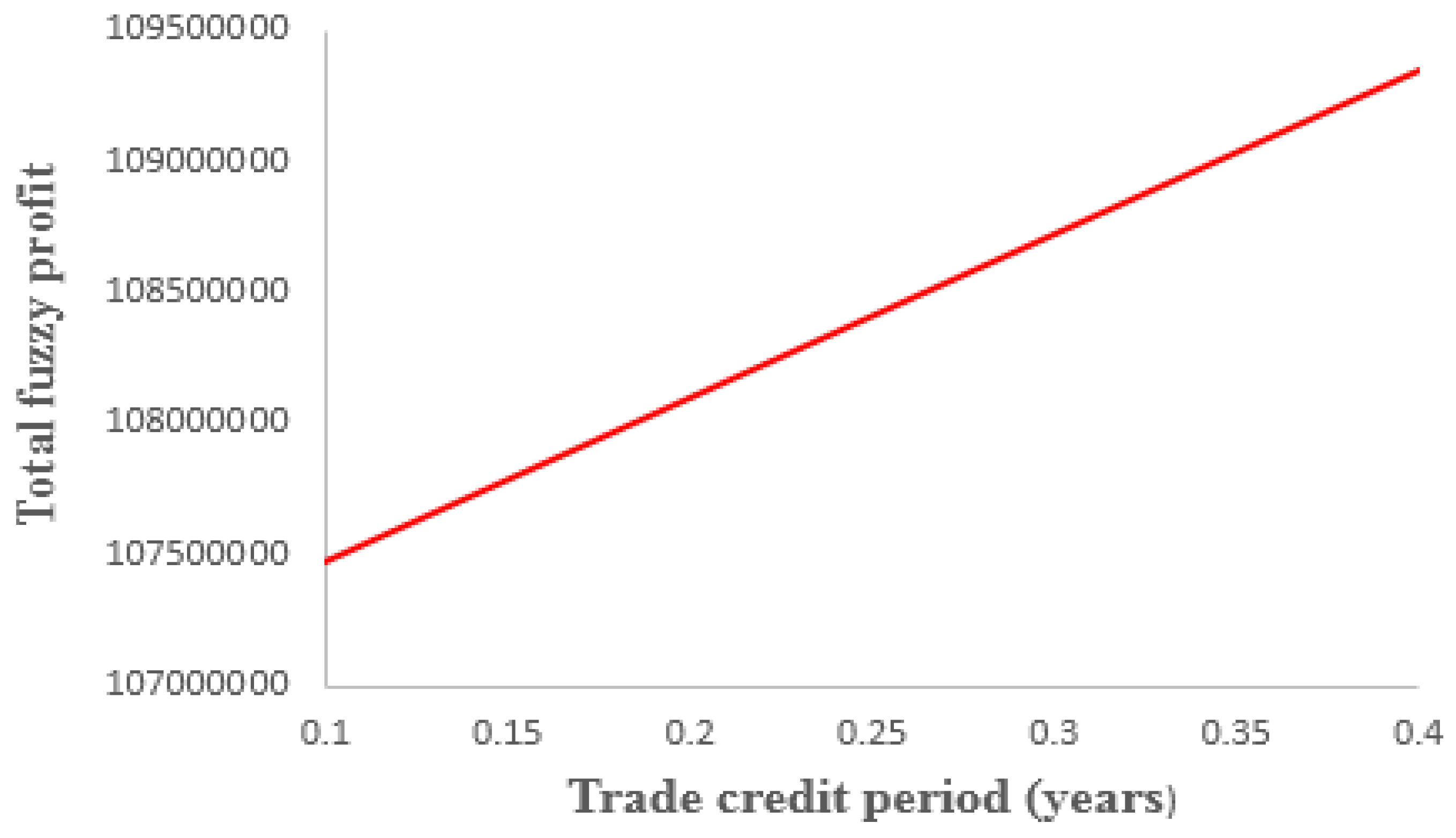
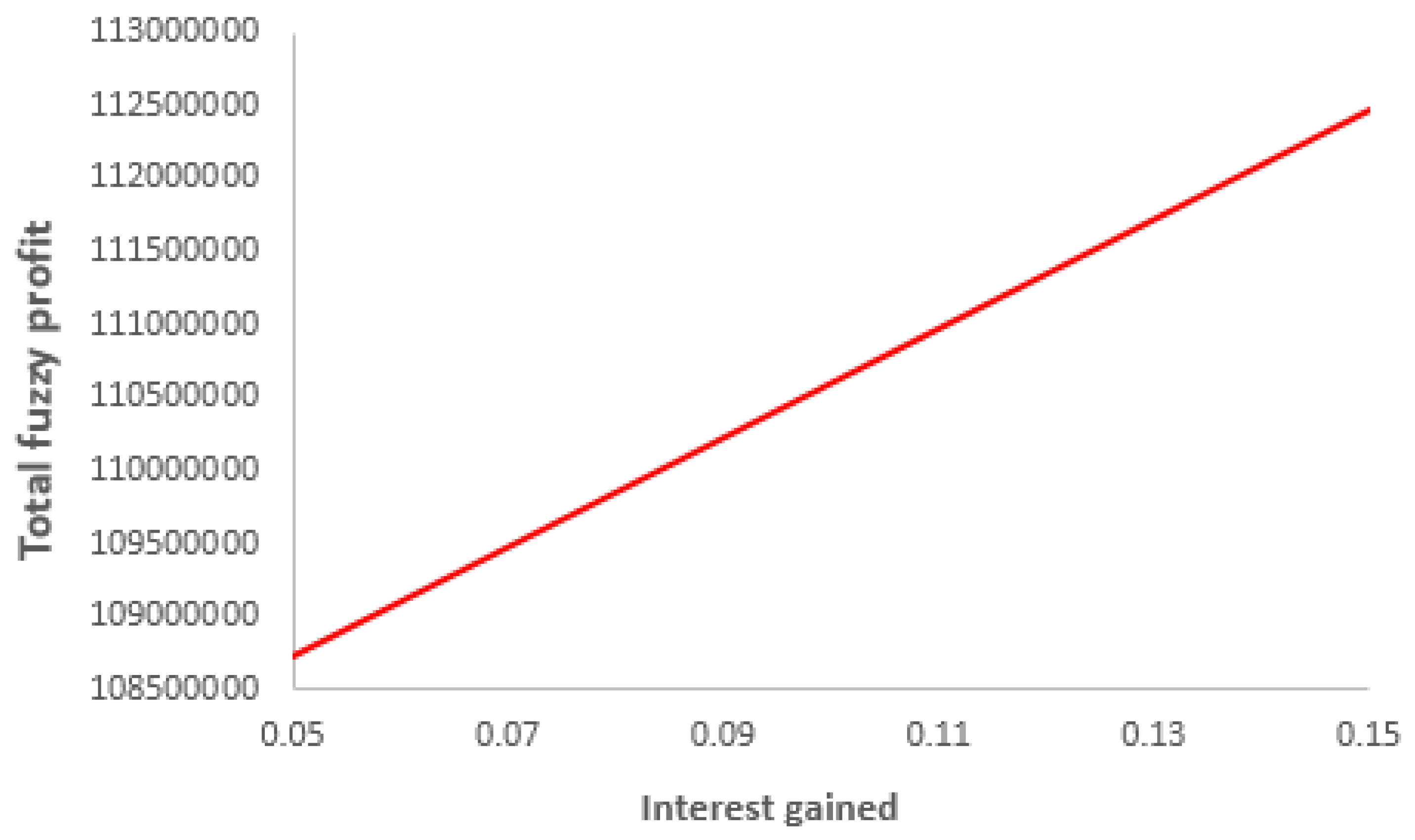
• From Table 5, it can be observed that when the credit period increases, the number of newborn items and the buyer’s total fuzzy profit increase as well. The newborn items and buyer’s total profit increase due to the presence of the trade credit policy because the buyer obtains more credit period for the selling of items, and its revenue generates more due to interest earned and the selling of items when trade credit period is less than or equal to cycle length. On the other hand, the seller obtains more profit due to interest paid when the buyer does not return borrowed items on or before the fixed credit period. Finally, in this model, the credit policy positively affects the order quantity and the buyer’s total fuzzy profit. The trade-credit policy can be risky for the seller when the financing period is very large. The graphical impact of the trade credit period has been shown in Figure 9 and Figure 10.
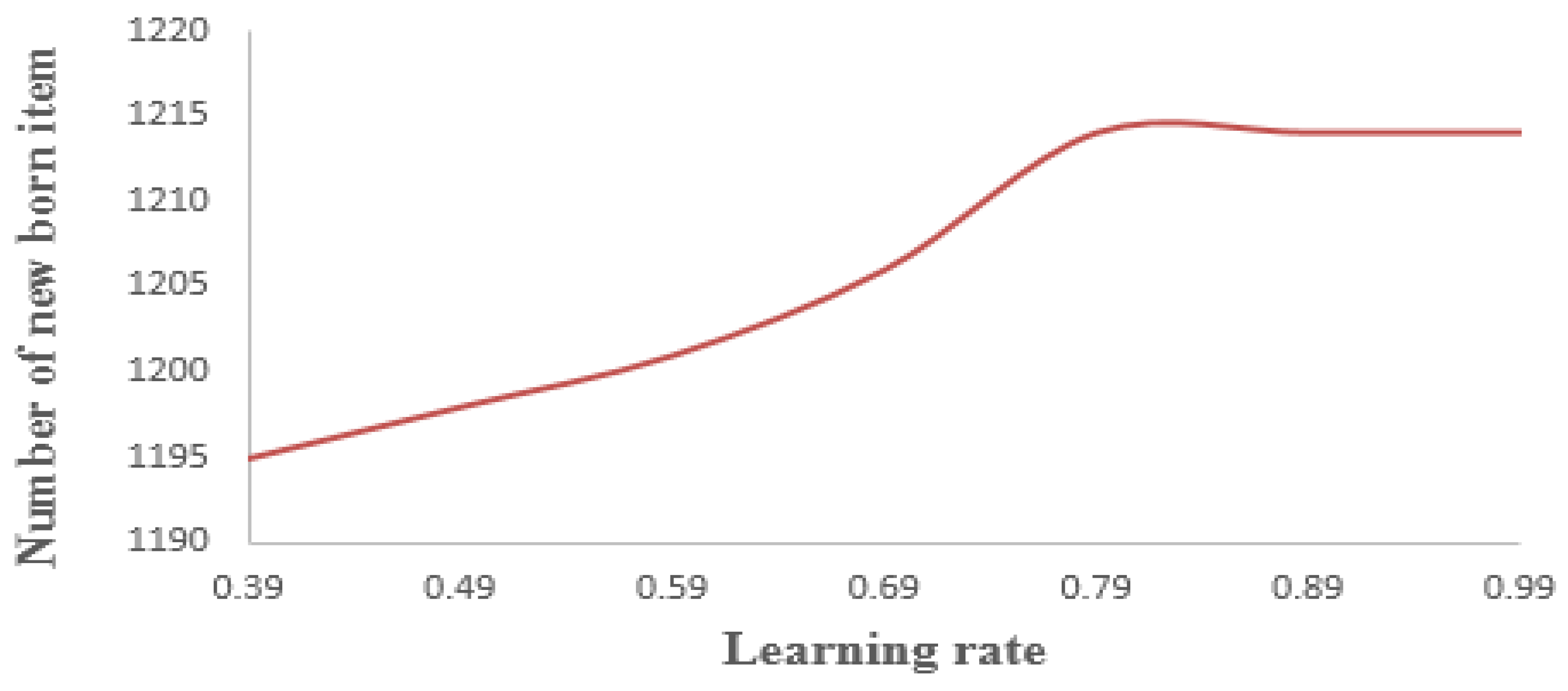
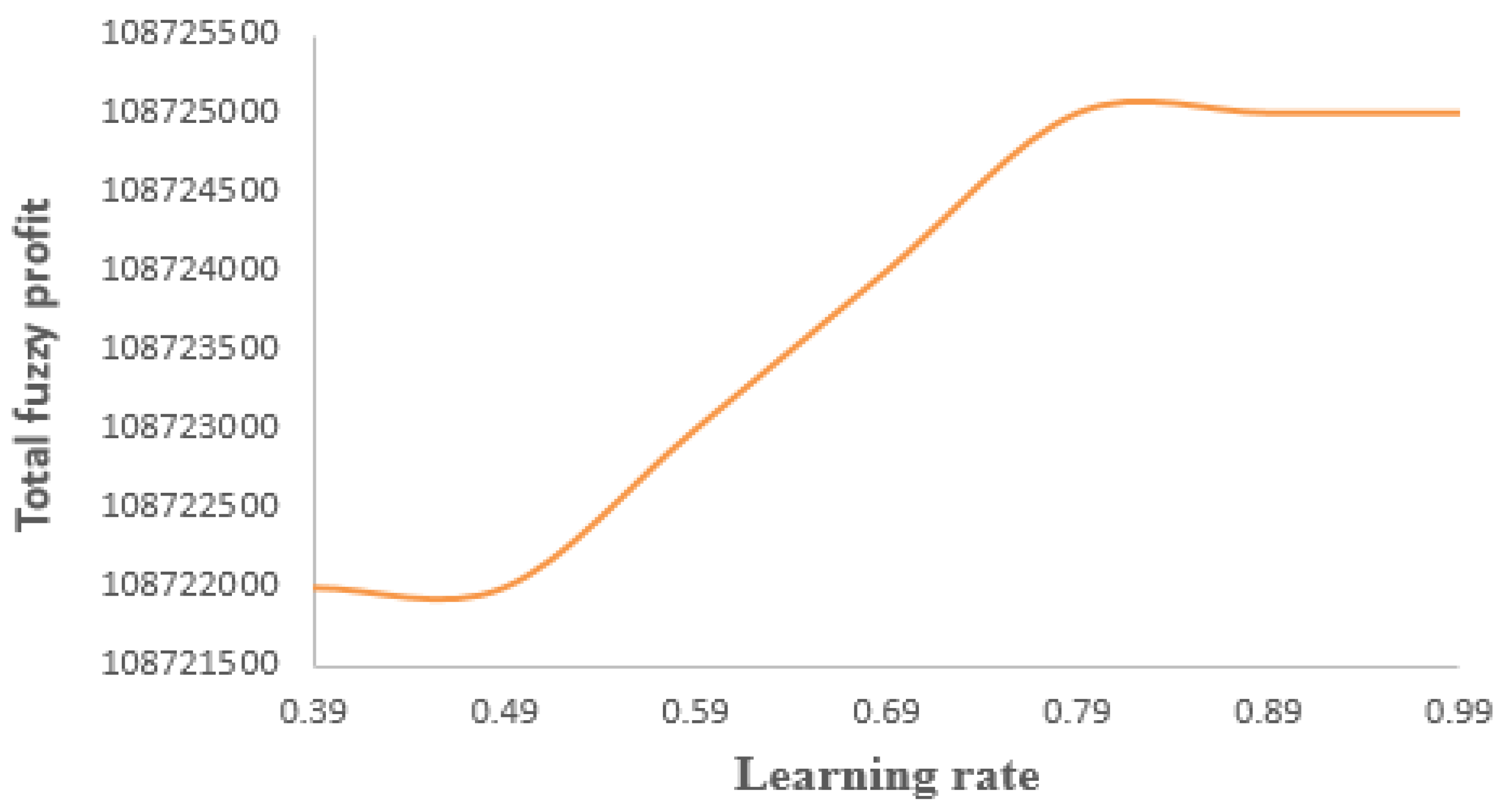
• From Table 6, it can be analyzed that as the learning rate increases with keeping other model parameter constant, the number of newborn items and the buyer’s total fuzzy profit increase because when the learning rate increases, the percentage of defective items decreases per shipment, but those items cannot be removed from the lot. Initially, the order quantity increases when the learning rate increases, but only for some time, and for some values of the learning rate, the order quantity becomes constant. This specific value of the learning rate is more important for the fishery industry and the order quantity. Learning theory suggests that the buyer obtains more profit on less order quantity. The impact of the learning rate has been shown in Figure 11 and Figure 12.
• From Table 7, if the lower and upper deviation of the fuzzy demand rate increase, the number of newborn items and the buyer’s total fuzzy profit increase because the selling of items increases and generates more revenue. The interest earned and interest paid vary due to the lower and upper deviation of the demand rate. The decision-makers can manage the value of the lower and upper deviation of the demand rate for the fishery industry. The fuzzy learning theory is more beneficial for the fishery industry.
• From Table 8, if the feeding cost increases, the number of newborn items is constant while the buyer’s total fuzzy profit decreases due to the addition of the feeding cost to the revenue cost.
• From Table 9, if the holding cost increases, the number of newborn items is constant while the buyer’s total fuzzy profit decreases because the cost function increases due to the increase in the holding cost.
• From Table 10, the inspection of the lot must be performed when the lot has some defective items. If the inspection cost $\left(I_s\right)$ increases, the number of newborn item is constant, whereas the buyer’s total profit decreases because the cost function increases. The decision-makers can manage the inspection cost according to the model.
• From Table 11, we see that if the purchasing cost increases, the number of newborn item is constant, and the buyer’s total fuzzy profit decreases because the cost function increases.
• From Table 12, when the buyer increases the selling price of good quality items, the number of newborn items is constant and increases the total fuzzy profit because the selling price of good items is more than the purchasing price and generates more revenue due to more sales.
• From Table 13, when the carbon emission tax rate increases, the number of newborn items is constant, but the buyer’s total fuzzy profit decreases due to the addition of carbon taxation in the cost function.
• From Table 14, if the traveling distance increases, then the number of the newborn items is constant, but the buyer’s total fuzzy profit decreases because the emission cost increases due to the increase in distance.

8. Conclusions

The present paper describes a supply chain model with carbon emissions and learning effect for the growing items (fishes) under a fuzzy environment and trade credit policy where the demand rate is taken as a triangular fuzzy number and defective items follow the S-shaped learning curve. The companies or firms need to optimize the inventory of newborn growing items (fishes, chicks, feeds, and extra). In this paper, we have optimized the buyer’s total fuzzy profit with respect to the number of newborn growing items (fishes), and the players (seller and buyer) of the supply chain obtained more profit under some realistic situations, such as the inspection of the lot, trade-credit policy, consideration of fuzzy demand rate, and the effect of the learning. We observed and analyzed some results from the behavior of the inventory parameters and briefly discussed them in the observation and managerial insights section. The inventory cost affects the total fuzzy profit of the supply chain’s members. The buyer obtained more profit in case 3 because the buyer does not pay extra interest charges and only earns gained interest as well as no pressure for selling the growing items while both players take benefits during the dealing of that contract under trade credit policy. From case 1 and case 2, we concluded that the buyer faces some difficulties in selling the items because he has to pay for the unsold items as per the contracted. From the sensitivity analysis of the inventory parameters, we conclude that the trade credit policy and learning fuzzy theory are more effective tools in this model, and these parameters directly affect the size of the newborn items and the buyer’s total profit. The seller should be aware of the trade credit when it plans to use the policy of trade credit, and without a plan, it can be riskier for the seller. The trade-credit policy is more effective when the demand for newborn items is constant, whereas, in this model, the demand for newborn items is uncertain. The buyer’s total fuzzy profit is defuzzified with the help of the signed distance method for the nullification of the uncertainty of the demand for newborn items. The present model suggests to the decision-makers that, at the time of ordering, one should be aware of the trade credit time, rate of learning, and deviation of lower and upper demand of newborn items. The learning rate suggests a minimum order quantity on which the buyer obtains more profit, and this model is developed especially for the fishery industry. We obtained some decision-making results from the sensitivity analysis of the learning rate when the learning rate is 0.79, and the order quantity and the buyer’s total fuzzy profit become saturated. The application of this research work is very important wherein a firm or a company purchases newborn fish, chicks, feeds, etc., after they are sold in another market when newborns have gained a certain weight. Companies or firms need to optimize the inventory of newborn growing items. The limitation of the paper is that the demand rate should be imprecise in nature, and the upper and lower deviation of the demand rate should be in the proper range. The rate of learning, shipments, and trade credit period should be checked before the strategy of mathematical modeling because these are changeable under some realistic situations. The proposed model can be improved with the contribution of Sarkar et al. [40], Bachar et al. [41], and Mondal et al. [42] for a closed-loop supply for greening defective items under some realistic situations. We obtained fruitful suggestions from the observation, and when the seller wishes to start a business for growing items, especially for newborn fishes, the seller must use the trade credit scheme to increase the selling of newborn items (fishes) in addition to new clients. The fuzzy learning theory is more effective when the demand for newborn items is uncertain. In the case of the fishery industry, the demand for newborn items is not constant, and sometimes it varies, and in this case, the buyer should use the concept of learning a fuzzy environment.

When a seller and buyer connect through a trade credit scheme and generate a supply chain for a long time of the demand for newborn items is uncertain and the carbon units emit during transportation. The contribution of this scenario is more useful because the uncertainty of the demand for newborn items can be nullified with the help of fuzzy theory, and learning suggests how much order quantity should be for newborn items during the transaction of business. Minimum carbon emission cost reduces the total cost of the supply chain, which results in higher profit for the supply chain partners. The contribution of this paper covers the area of the topic of reputed journals, and it will be very helpful for the fishery industry.

References

1. Harris, F.W. How many parts to make at once. Factory Mag. Manag. 1913, 10, 135–136. [Google Scholar] [CrossRef]
2. Aggarwal, S.P.; Jaggi, C.K. Ordering policies of deteriorating items under allowable deferment in payments. J. Oper. Res. Soc. 1995, 46, 658–662. [Google Scholar] [CrossRef]
3. Chu, P.; Chung, K.J.; Lan, S.P. Economic order quantity of deteriorating items under allowable deferment in payments. Comput. Oper. Res. 1998, 25, 817–824. [Google Scholar] [CrossRef]
4. Abad, P.L.; Jaggi, C.K. A joint approach for setting unit price and the length of the credit period for a supplier when end demand is price sensitive. Int. J. Prod. Econ. 2003, 83, 115–122. [Google Scholar] [CrossRef]
5. Chung, K.J.; Liao, J.J. The optimum ordering policy in a DCF analysis for deteriorating items when trade credit depends on the order quantity. Int. J. Prod Econ. 2006, 100, 116–130. [Google Scholar] [CrossRef]
6. Salameh, M.K.; Jaber, M.Y. Economic production quantity model for items with imperfect quality. Int. J. Prod. Econ. 2000, 64, 59–64. [Google Scholar] [CrossRef]
7. Chung, K.J.; Her, C.C.; Lin, S.D. A two warehouse inventory model with imperfect quality production process. Comput. Ind. Eng. 2009, 56, 193–197. [Google Scholar] [CrossRef]
8. Huang, C.K. An integrated vendor–buyer cooperative inventory model for items with imperfect quality. Prod. Planning Control 2002, 13, 355–361. [Google Scholar] [CrossRef]
9. Jaber, M.Y.; Goyal, S.K.; Imran, M. Economic production quantity model for items with imperfect quality subject to learning effects. Int. J. Prod. Econ 2008, 115, 143–150. [Google Scholar] [CrossRef]
10. Jaggi, C.K.; Khanna, A.; Mittal, M. Credit financing for deteriorating imperfect-quality items under inflationary conditions. Int. J. Serv. Oper. Inf. 2011, 6, 292–309. [Google Scholar] [CrossRef]
11. Zhang, L.; Li, Y.; Tian, X.; Feng, C. Inventory management research for growing items with carbon constrained. In Proceedings of the 2016 35th Chinese Control Conference (CCC), Chengdu, China, 27–29 July 2016; pp. 9588–9593. [Google Scholar]
12. Tiwari, S.; Daryanto, Y.; Wee, H.M. Sustainable inventory management with deteriorating and imperfect quality items considering carbon emission. J. Clean Pro. 2018, 192, 281–292. [Google Scholar] [CrossRef]
13. Sebatjane, M.; Adetunji, O. Economic order quantity model for growing items with imperfect quality. Oper. Res. Perspect. 2019, 6, 100088. [Google Scholar] [CrossRef]
14. De-la-Cruz-Marquez, C.G.; Cardenas-Barron, L.E.; Mandal, B. An inventory model for growing items with imperfect quality when the demand is price sensitive under carbon emissions and shortages. Math. Prob. Eng. 2021, 2021, 1–23. [Google Scholar] [CrossRef]
15. Chang, H.C. An application of fuzzy sets to the EOQ model with imperfect quality items. Comput. Oper. Res. 2004, 31, 2079–2092. [Google Scholar] [CrossRef]
16. Rani, S.; Ali, R.; Agarwal, A. Fuzzy inventory model for new and refurbished deteriorating items with cannibalization in green supply chain. Int. J. Syst. Sci. Oper. Logist. 2022, 9, 22–38. [Google Scholar]
17. Wright, T.P. Factors affecting the cost of airplanes. J. Aero. Sci. 1936, 3, 122–128. [Google Scholar] [CrossRef]
18. Wee, H.M.; Yu Chen, M.C. Optimum inventory model for items with imperfect quality and shortage backordering. Omega 2007, 35, 7–11. [Google Scholar] [CrossRef]
19. Jayaswal, M.K.; Mittal, M.; Sangal, I. Ordering policies for deteriorating imperfect quality items with trade-credit financing under learning effect. Int. J. Syst. Assur. Eng. Manag. 2021, 12, 112–125. [Google Scholar] [CrossRef]
20. Jayaswal, M.; Sangal, I.; Mittal, M.; Malik, S. Effects of learning on retailer ordering policy for imperfect quality items with trade credit financing. Uncertain Supp. Chain Manag. 2019, 7, 49–62. [Google Scholar] [CrossRef]
21. Alamri, O.A.; Jayaswal, M.K.; Khan, F.A.; Mittal, M. An EOQ Model with Carbon Emissions and Inflation for Deteriorating Imperfect Quality Items under Learning Effect. Sustainability 2022, 14, 1365. [Google Scholar] [CrossRef]
22. Jayaswal, M.K.; Mittal, M.; Alamri, O.A.; Khan, F.A. Learning EOQ Model with Trade-Credit Financing Policy for Imperfect Quality Items under Cloudy Fuzzy Environment. Mathematics 2022, 10, 246. [Google Scholar] [CrossRef]
23. Rezaei, J. Economic order quantity for growing items. Int. J. Prod. Econ. 2014, 155, 109–113. [Google Scholar] [CrossRef]
24. Mittal, M.; Sharma, M. Economic ordering policies for growing items (poultry) with trade-credit financing. Int. J. Appl. Comput. Math. 2021, 7, 39. [Google Scholar] [CrossRef]
25. Pattnaik, S. Linearly Deteriorating EOQ Model for Imperfect Items with Price Dependent Demand Under Different Fuzzy Environments. Turk. J. Comput. Math Educ. 2021, 12, 5328–5349. [Google Scholar]
26. Rajeswari, S.; Sugapriya, C.; Nagarajan, D.; Kavikumar, J. Optimization in fuzzy economic order quantity model involving pentagonal fuzzy parameter. Inte. J. Fuz. Sys. 2022, 24, 44–56. [Google Scholar] [CrossRef]
27. Mahapatra, A.S.; Mahapatra, M.S.; Sarkar, B.; Majumder, S.K. Benefit of preservation technology with promotion and time-dependent deterioration under fuzzy learning. Expert Syst. Appl. 2022, 201, 117169. [Google Scholar] [CrossRef]
28. Taheri, J.; Mirzazadeh, A. Optimization of inventory system with defects, rework failure and two types of errors under crisp and fuzzy approach. J. Ind. Manag. Optim. 2022, 18, 2289–2318. [Google Scholar] [CrossRef]
29. Dinagar, D.S.; Manvizhi, M. Single-Stage Fuzzy Economic Inventory Models with Backorders and Rework Process for Imperfect Items. J. Algebraic Stat. 2022, 13, 3008–3020. [Google Scholar]
30. Garg, H.; Sugapriya, C.; Kuppulakshmi, V.; Nagarajan, D. Optimization of fuzzy inventory lot-size with scrap and defective items under inspection policy. Sot. Comput. 2023, 27, 2231–2250. [Google Scholar] [CrossRef]
31. Kuppulakshmi, V.; Sugapriya, C.; Kavikumar, J.; Nagarajan, D. Fuzzy Inventory Model for Imperfect Items with Price Discount and Penalty Maintenance Cost. Math. Prob. Engin. 2023, 2023, 1–15. [Google Scholar] [CrossRef]
32. Jayaswal, M.K.; Mittal, M. Impact of Learning on the Inventory Model of Deteriorating Imperfect Quality Items with Inflation and Credit Financing under Fuzzy Environment. Int. J. Fuzzy Syst. Appl. 2022, 11, 1–36. [Google Scholar] [CrossRef]
33. Chung, K.J.; Huang, Y.F. Retailer’s optimal cycle times in the EOQ model with imperfect quality and a permissible credit period. Qual. Quant. 2006, 40, 59–77. [Google Scholar] [CrossRef]
34. Sulak, H. An EOQ model with defective items and shortages in fuzzy sets environment. Int. J. Soc. Sci. Educ. Res. 2015, 2, 915–929. [Google Scholar] [CrossRef]
35. Shekarian, E.; Olugu, E.U.; Abdul-Rashid, S.H.; Kazemi, N. An economic order quantity model considering different holding costs for imperfect quality items subject to fuzziness and learning. J. Intell. Fuz. Syst. 2016, 30, 2985–2997. [Google Scholar] [CrossRef]
36. Kazemi, N.; Abdul-Rashid, S.H.; Ghazilla RA, R.; Shekarian, E.; Zanoni, S. Economic order quantity models for items with imperfect quality and emission considerations. Int. J. Syst. Sci. Oper. Logist. 2018, 5, 99–115. [Google Scholar] [CrossRef]
37. Alsaedi, B.S.; Alamri, O.A.; Jayaswal, M.K.; Mittal, M. A Sustainable Green Supply Chain Model with Carbon Emissions for Defective Items under Learning in a Fuzzy Environment. Mathematics 2023, 11, 301. [Google Scholar] [CrossRef]
38. Jaggi, C.K.; Goel, S.K.; Mittal, M. Credit financing in economic ordering policies for defective items with allowable shortages. Appl. Math. Compt. 2013, 219, 5268–5282. [Google Scholar] [CrossRef]
39. Gurtu, A.; Jaber, M.Y.; Searcy, C. Impact of fuel price and emissions on inventory policies. Appl. Math. Model. 2015, 39, 1202–1216. [Google Scholar] [CrossRef]
40. Sarkar, B.; Ganguly, B.; Pareek, S.; Cárdenas-Barrón, L.E. A three-echelon green supply chain management for biodegradable products with three transportation modes. Comput. Ind. Eng. 2022, 174, 108727. [Google Scholar] [CrossRef]
41. Bachar, R.K.; Bhuniya, S.; Ghosh, S.K.; Sarkar, B. Controllable Energy Consumption in a Sustainable Smart Manufacturing Model Considering Superior Service, Flexible Demand, and Partial Outsourcing. Mathematics 2022, 10, 4517. [Google Scholar] [CrossRef]
42. Mondal, A.K.; Pareek, S.; Chaudhuri, K.; Bera, A.; Bachar, R.K.; Sarkar, B. Technology license sharing strategy for remanufacturing industries under a closed-loop supply chain management bonding. RAIRO Oper. Res. 2022, 56, 3017–3045. [Google Scholar] [CrossRef]
Figure 1. Representation of model’s flowchart.
Axioms 12 00436 g001
Figure 2. Membership function of a triangular fuzzy number.
Axioms 12 00436 g002
Figure 3. S-Shape learning curve.
Axioms 12 00436 g003
Figure 4. Model presentation under logistic growth function.
Axioms 12 00436 g004
Figure 5. Model presentation under logistic growth function and credit policy scheme.
Axioms 12 00436 g005
Figure 6. Model presentation under logistic growth function for the case 0 M t 2 .
Axioms 12 00436 g006
Figure 7. Model presentation under logistic growth function for the case t 2 M T .
Axioms 12 00436 g007
Figure 8. Model presentation under logistic growth function for the case t 2 T M .
Axioms 12 00436 g008
Figure 9. Effect of the trade credit period on the total fuzzy profit.
Axioms 12 00436 g009
Figure 10. Effect of the interest gained on the total fuzzy profit.
Axioms 12 00436 g010
Figure 11. Effect of the learning rate on the number of newborn items.
Axioms 12 00436 g011
Figure 12. Effect of the learning rate on the total fuzzy profit.
Axioms 12 00436 g012