

Spectral Properties of Exact Polarobreathers in Semiclassical Systems


Abstract
:1. Introduction
2. The Model
3. Frequency Shift of the Charge Amplitudes
4. Review of the Properties of Exact Moving Breathers and Solitons
- Exact traveling wave:
- An exact traveling wave with velocity is characterized by a function or sum of functions of the form:with f a periodic on its second one, and with the following condition below.
- Fundamental time and step:
- There exist a fundamental time and an integer number called the step s, so the profile f repeats exactly after a time . The velocity is then .
- Localized solutions:
- If f is localized in the first variable, it may be a breather, soliton, or kink. We will refer to it as a breather for simplicity. Then, we write the second variable as . If it is delocalized, it is an exact extended traveling wave.
- Fundamental frequency:
- . The relevant frequencies are integer multiples of , among which is the frequency associated to the velocity, i.e., the frequency at which a traveler in the moving frame encounters particles .
- Frequency in the moving frame:
- is the frequency in the moving frame, because if an observer moves with the breather, then , and there remains a single frequency , for the breather. We do not take into account the variation due to the discreteness.
- Exactness:
- The exactness condition implies that for the integer m, or for the breather.
- Harmonic modes:
- The breather, as any function of , can be expressed as a sum of harmonic waves, also called modes , with being the laboratory frequency of each mode.
- Resonant modes:
- Resonant modes with the breather are all the modes that advance the step s in the time , that is, they are also exact with the same step and fundamental frequency. They can be written as .
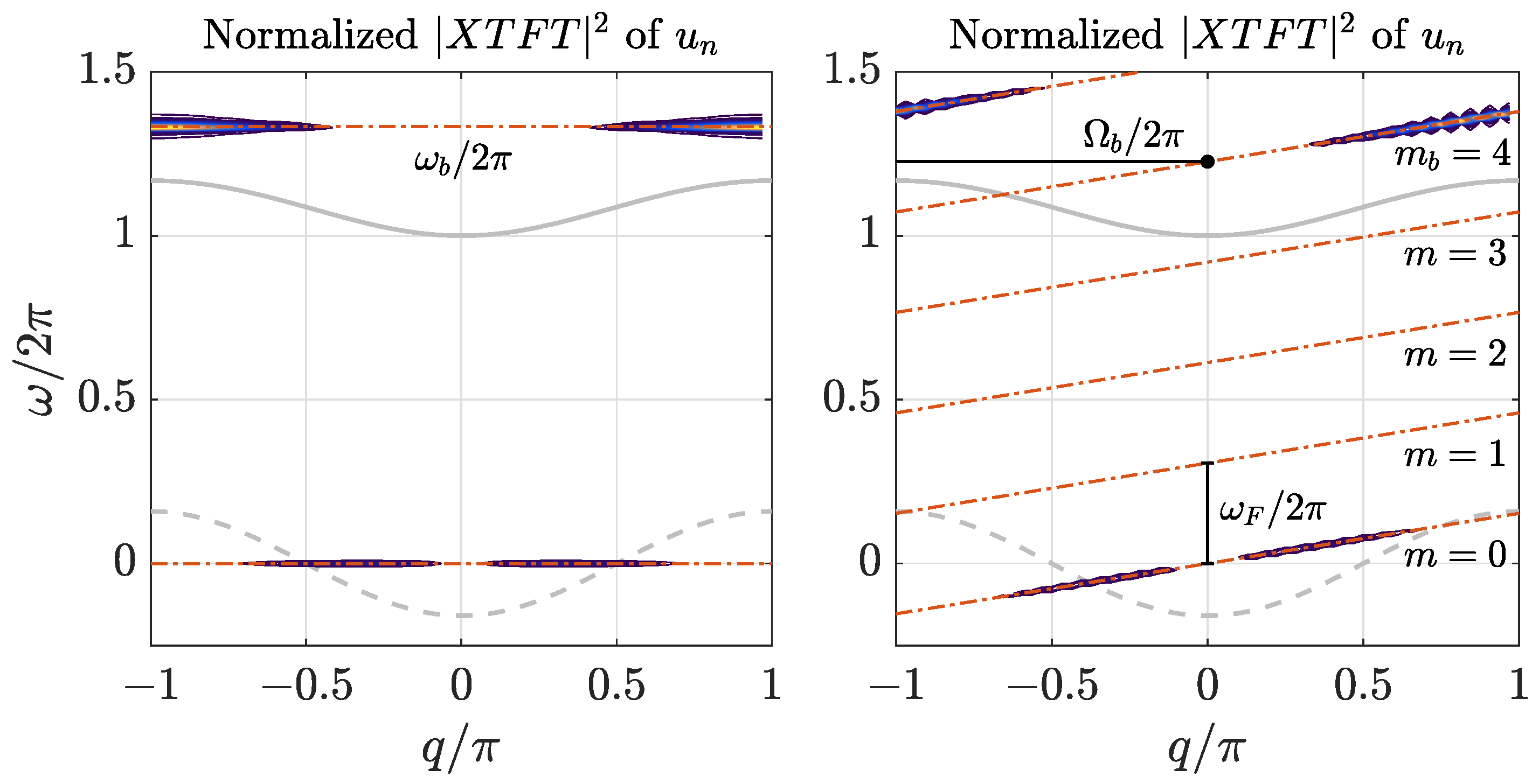
- Resonant lines:
- Therefore, the laboratory frequencies of the resonant modes are given by . They form parallel straight lines called resonant lines, with slope , and cross the vertical axis () at , for the m integer. All modes in a resonant line travel with speed and have the same frequency in the moving frame .
- Breather line:
- All the modes in the spectrum of the localized exact solution are within one resonant line, with , that is, the breather line. Note that the breather line ends at and reappears at as a different resonant line.
- Breather frequency in the moving frame:
- The breather line crosses the vertical axis () at , the frequency of the breather in the moving frame.
- Transformation to the moving frame:
- Changing the frame of reference to the one moving with the breather, it is equivalent to the transformation . The resonant lines and the breather line become horizontal lines with the frequencies in the moving frame.
- Soliton or kink:
- If , the excitation is a kink or soliton, that is, a static profile in the moving frame.
- Wing:
- If a resonant line crosses the dispersion band, there is a resonant phonon, i.e., a solution to the linearized equation, that may bring about a wing. It is an extended wave that travels with the localized solution, becoming a pterobreather, pterosoliton, or pterokink. The wing may be an integral part of the solution to the nonlinear dynamical equations, that is, it will not exist without the wing [42].
- Commensurability condition:
- The breather line frequency change for is , the velocity frequency, which is given by . Then,is a rational number. This important property allows for the determination of , s, , , and , by simple inspection of the breather spectrum. is also the difference in frequency between the breather line and its continuation when . The moving frame frequency and the velocity frequency are commensurate.
5. Linear Approximations
6. Tail Analysis of Stationary Localized Excitations
7. Tail Analysis of Moving Localized Excitations
8. Numerical Methods
8.1. Numerical Integration of the Canonical Hamiltonian Equations
8.2. Numerical Algorithm for Computation of Exact Polarobreathers

9. Stationary Polarobreathers
9.1. Generation of Approximate Stationary Polarobreathers
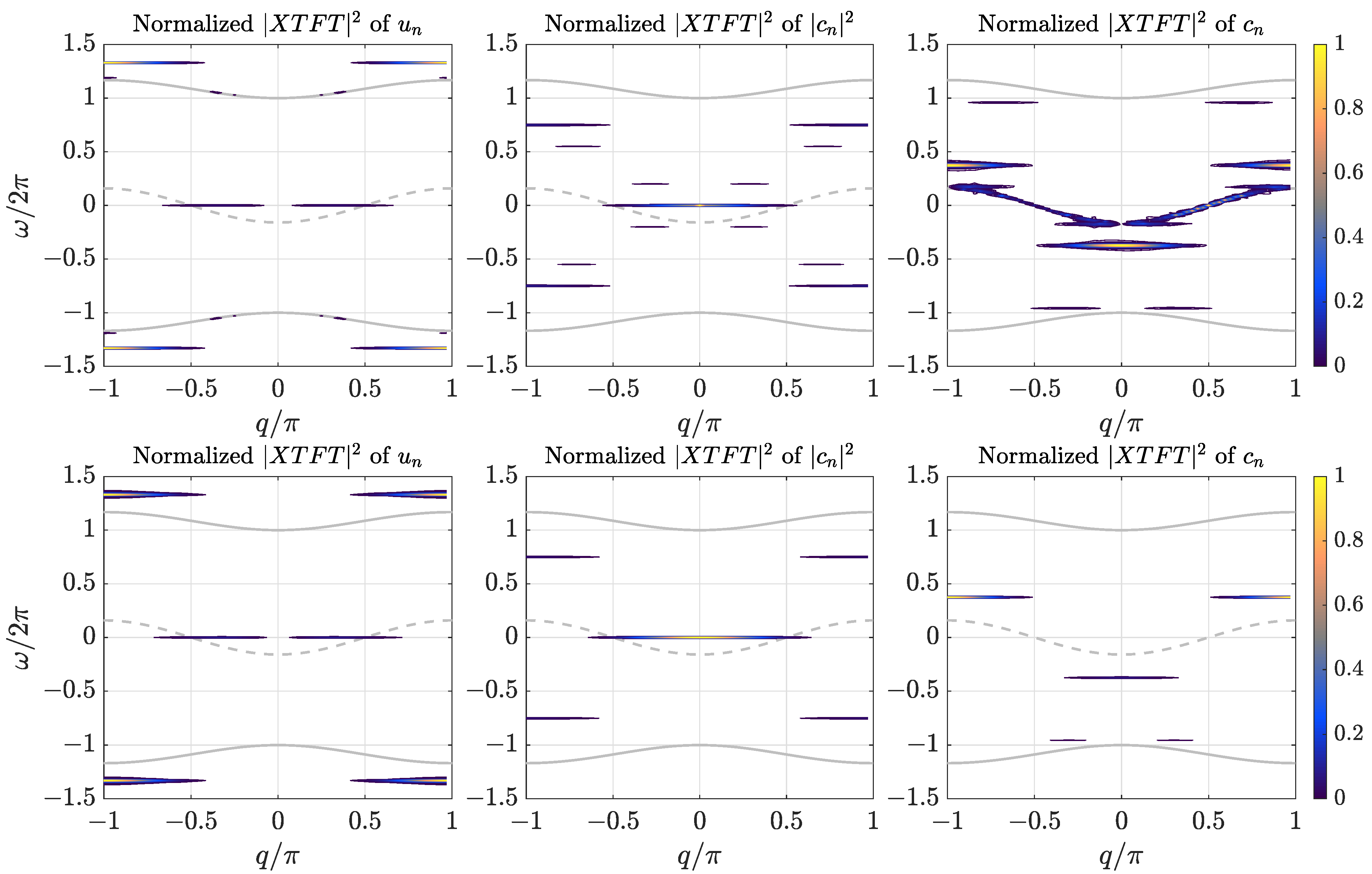
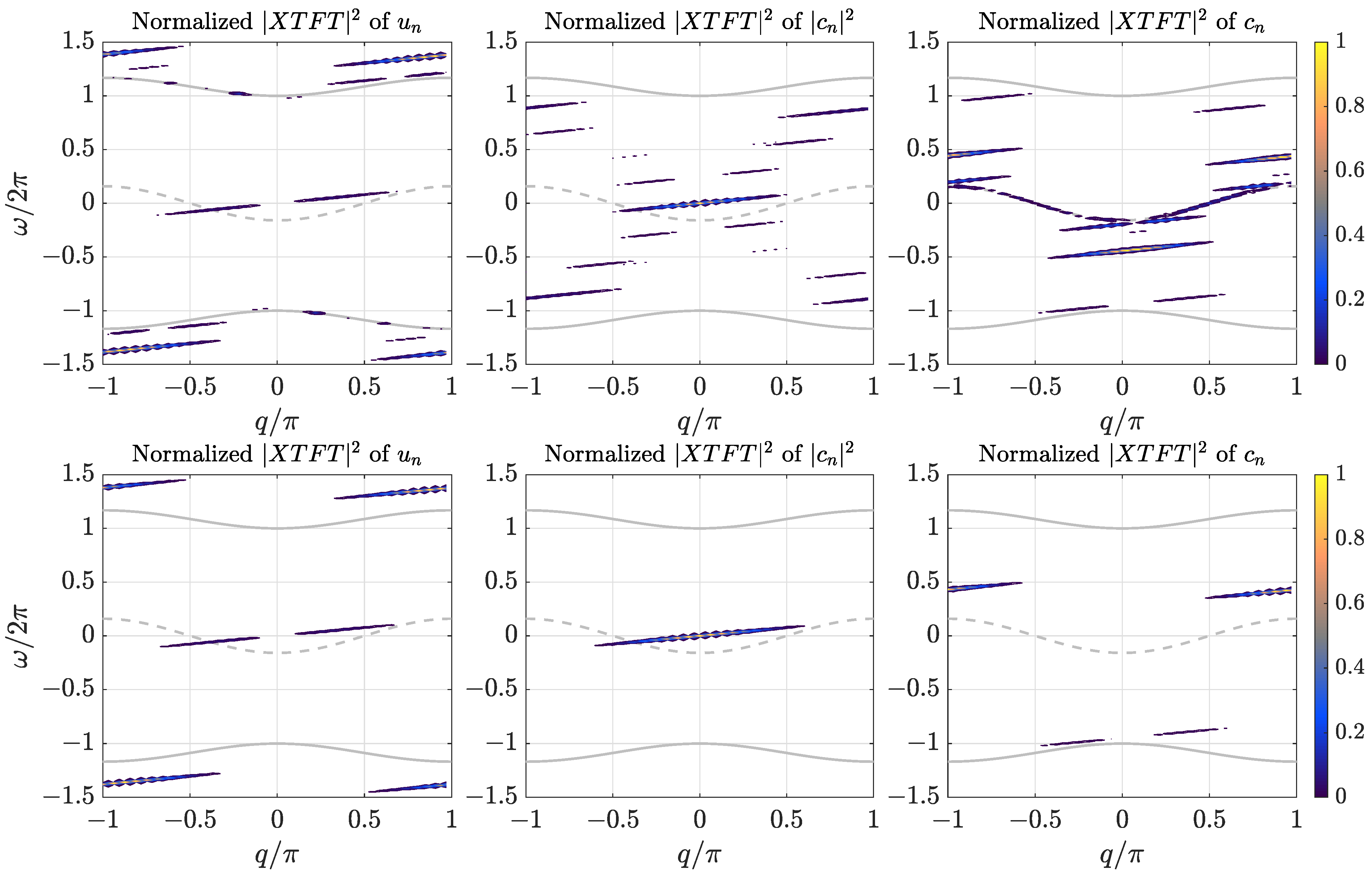
- For the of , there appear two horizontal lines at , centered around , and some frequency above the dispersion relation and centered around . This means that the breather is composed of a soliton, that is, a static deformation with a displacement largely in phase and a staggered vibration above the phonon spectrum, i.e., a nonlinear vibration, as demonstrated in Section 6. The static solution appears due to the asymmetry of the Lennard-Jones potential well, which makes compression harder than expansion, and therefore, oscillations with respect to the equilibrium distance are larger for expansion than for compression.
- For , two horizontal lines appear, one at zero frequency, a stationary soliton close to , that is, with nearest neighbors in phase; and also at frequency , close to the modes , that is, with a staggered profile. The soliton here is necessary, as is a positive quantity, so the vibration has an alternating pattern around a stationary one. This means that there is a small change in probability between neighboring particles with the frequency . This was also explained in Section 6. Depending on the nonlinearity and the system, the interchange of probability will be larger or smaller.
- For , we find three main frequencies, two of them , close to the phonon spectrum, one above and the other below. The upper one is around , i.e., with a staggered profile; and the lower one is around , that is, with a bell profile. These two frequencies are explained in Section 6. The other two are located at . These appear because the quantum Hamiltonian has the time periodicity of , which appears in the transfer matrix elements.
- There are some other lines of weaker intensity in of , but especially for . We can observe some phonons for and even more for , where they occupy the whole -phonon band, but not for , as there is no dispersion relation for , because its evolution depends on the other terms of the density matrix [40]. Results on the density matrix for polarobreathers will be discussed and published elsewhere.
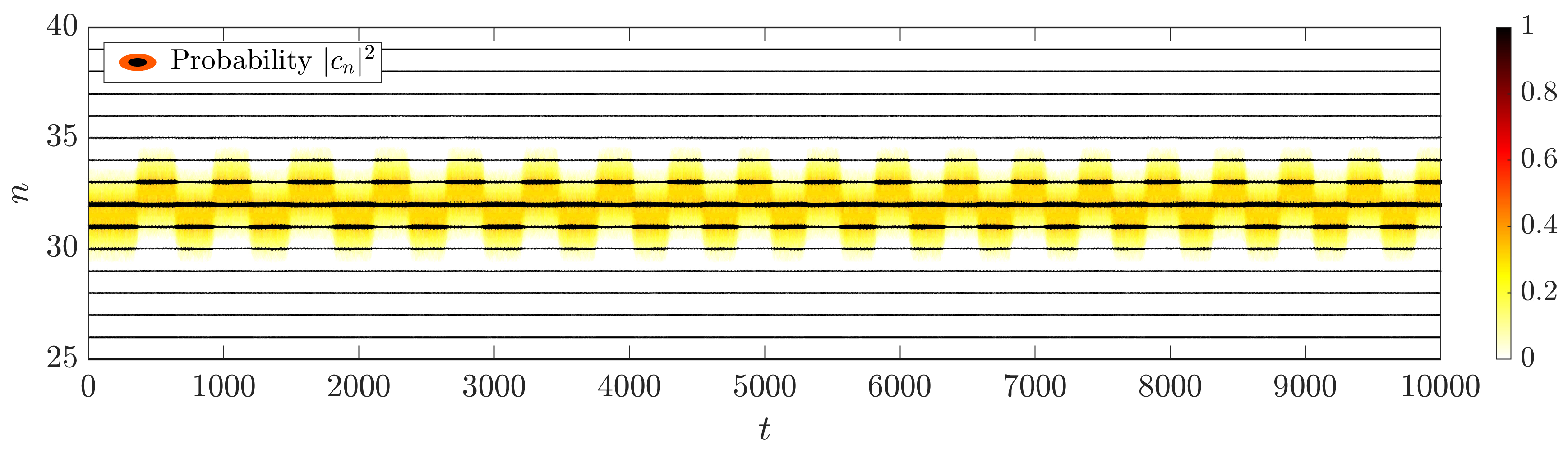
9.2. Exact Stationary Polarobreathers
- All the phonons have disappeared from the dispersion bands.
- Extra bands have also disappeared, except for the ones described above, which have become much more defined.
- In the of , the zero-frequency component corresponding to the stationary soliton and the frequency slightly above the positive phonon band, centered at (also the symmetric band at ), have remained. These features are in accordance with the theory described in Section 6.
- In the of , already shifted to by the numerically found value, only two bands— slightly above the phonon band at and below at , which correspond to a hard potential case—have remained; see Section 6.
- Furthermore, for the of , there is a weak negative frequency corresponding to the forcing by the matrix transfer elements , which change with , the frequency. The corresponding band is symmetric in q, but does not include . This means that it is a stationary wave: the sum of waves traveling in opposite directions with wavenumbers around or wavelength . With greater initial kinetic energy, the positive frequencies also appear above the positive phonon band and are centered at .
- In the plot of charge probability , only the bands with frequencies at zero and have remained, due to the election of , (as well as , due to the symmetry).
9.3. Stability of Exact Stationary Solutions: The Switching Mode
10. Moving Polarobreathers
10.1. Generation of Approximate Moving Polarobreathers
- We observe the of . There are three localized waves traveling at the same speed, and some phonons. The three localized waves are a soliton; a breather; and with weaker intensity, what we could call a quasilinear breather, very close to the phonon band. We know that the soliton and main breather are characteristic components of this system, with strong asymmetry in the coupling potential. Therefore, we discard the weaker breather as an effect of the breather not being exact. In Section 4 it is deduced that the breather frequency in the moving frame is the frequency of the breather line for . The commensurability relation (17) was also obtained:with and the step being the integers we have to find. We measure and ; then . Therefore, the simplest values are
- For the of , also for positive frequencies, we observe four resonant lines with intensity. One is the soliton, characteristic of the of a positive quantity. The many lines are a sign of high nonlinearity, which corresponds to a very localized , and is therefore close to one for some n. The linear approximation is not at all valid, and there are many harmonic frequencies.
- For the of , we have to observe the frequency differences, as the solution is invariant to a global shift in frequency, as explained in Section 3. We observe many phonons in the dispersion band, two positive bands centered around , and two negative bands centered at . Two bands are very close to the phonon band, indicating a strong interaction with the linear modes. Observing the two truly nonlinear bands, their difference in frequency is , corresponding to . Using the commensurability relation (17) as above and with the same , we obtain:We conclude thatThus, we can set the common step and estimate the fundamental time , i.e.,as well as finding an approximate value of for the computation of the exact moving polarobreathers of the following section.
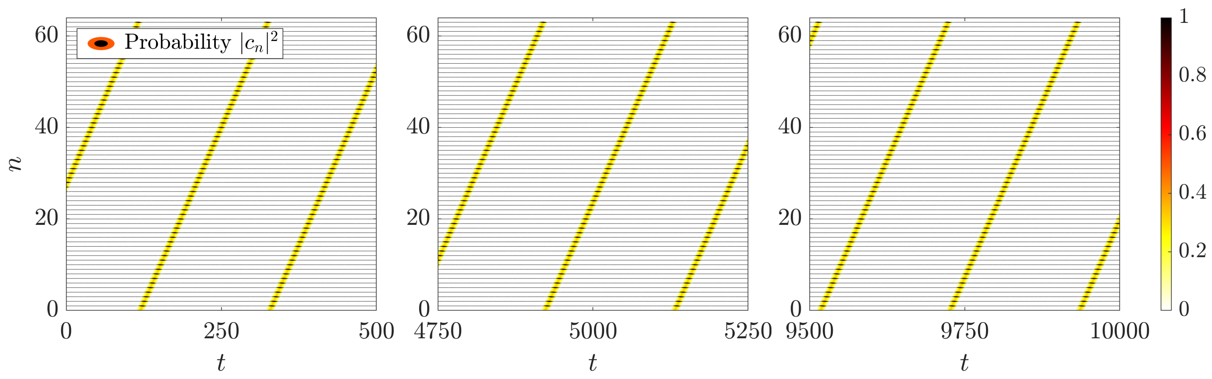
10.2. Exact Moving Polarobreathers
- For the of , phonons have been eliminated, and only a well localized soliton breather remains.
- For the of , only a soliton remains, meaning that in the moving frame, it is reduced to a static deformation, corresponding to a charge probability traveling without vibration. The other part of the solution is a uniform probability spread through the lattice, indicating a small probability that the charge could appear at any site n.
- For the of , two intensity bands remain: one around , and a stronger one centered at . The difference in frequencies is exactly the breather frequency, indicating that there is no vibration of , except the one driven by the change in the transfer elements , which depend on .
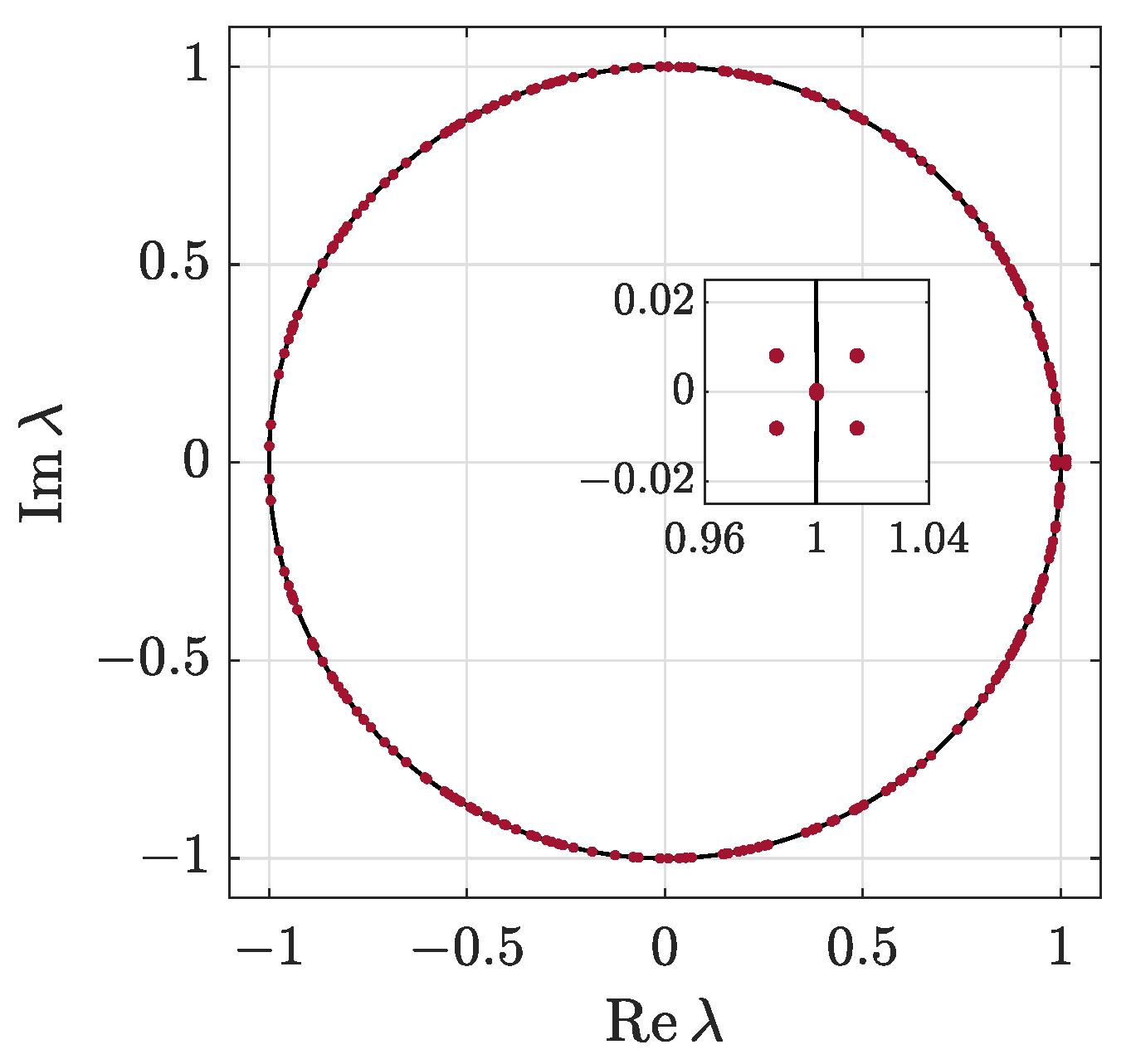
10.3. Stability of Moving Polarobreathers
10.4. Path Continuation
11. Conclusions
Author Contributions
Funding
Institutional Review Board Statement
Informed Consent Statement
Data Availability Statement
Conflicts of Interest
References
- Landau, L.D. Electron motion in crystal lattices. Phys. Z. Sowjetunion 1933, 3, 664. [Google Scholar]
- Landau, L.D.; Pekar, S.I. Effective mass of a polaron. Zh. Eksp. Teor. Fiz. 1948, 18, 419–423, English translation: Ukr. J. Phys. 2008, 53, 71–74. [Google Scholar]
- Holstein, T. Studies of polaron motion: Part I. The molecular-crystal model. Ann. Phys. 1959, 8, 325–342. [Google Scholar] [CrossRef]
- Holstein, T. Studies of polaron motion: Part II. The “small” polaron. Ann. Phys. 1959, 8, 343–389. [Google Scholar] [CrossRef]
- Alexandrov, A.S. Polarons in Advanced Materials; Springer: Dordrecht, The Netherlands, 2007. [Google Scholar]
- Dubinko, V.I.; Selyshchev, P.A.; Archilla, J.F.R. Reaction-rate theory with account of the crystal anharmonicity. Phys. Rev. E 2011, 83, 041124. [Google Scholar] [CrossRef] [Green Version]
- Davydov, A.S. Solitons in Molecular Systems; Mathematics and Its Applications; Springer: Dordrecht, The Netherlands, 1985. [Google Scholar]
- Remoissenet, M. Waves Called Solitons; Advanced Texts in Physics; Springer: Berlin, Germany, 1999. [Google Scholar]
- Sievers, A.J.; Takeno, S. Intrinsic Localized Modes in Anharmonic Crystals. Phys. Rev. Lett. 1988, 61, 970–973. [Google Scholar] [CrossRef]
- Sato, M.; Sievers, A.J. Direct observation of the discrete character of intrinsic localized modes in an antiferromagnet. Nature 2004, 432, 486–488. [Google Scholar] [CrossRef]
- Flach, S.; Gorbach, A.V. Discrete breathers. Advances in theory and applications. Phys. Rep. 2008, 467, 1–116. [Google Scholar] [CrossRef]
- MacKay, R.S.; Aubry, S. Proof of Existence of Breathers for Time-Reversible or Hamiltonian Networks of Weakly Coupled Oscillators. Nonlinearity 1994, 7, 1623. [Google Scholar] [CrossRef]
- Marín, J.L.; Aubry, S. Breathers in Nonlinear Lattices: Numerical Calculation from the Anticontinuous Limit. Nonlinearity 1996, 9, 1501. [Google Scholar] [CrossRef]
- Aubry, S. Breathers in nonlinear lattices: Existence, linear stability and quantization. Physica D 1997, 103, 1–4. [Google Scholar] [CrossRef]
- MacKay, R.S.; Sepulchre, J.A. Stability of discrete breathers. Physica D 1998, 119, 148–162. [Google Scholar] [CrossRef]
- Yoshimura, K.; Doi, Y. Moving discrete breathers in nonlinear lattice: Resonance and stability. Wave Motion 2007, 45, 83–99. [Google Scholar] [CrossRef]
- Butt, I.A.; Wattis, J.A.D. Asymptotic analysis of combined breather-kink modes in a Fermi-Pasta-Ulam chain. Physica D 2007, 231, 165–179. [Google Scholar] [CrossRef] [Green Version]
- Chong, C.; Kevrekidis, P.G.; Theocharis, G.; Daraio, C. Dark breathers in granular crystals. Phys. Rev. E 2013, 87, 042202. [Google Scholar] [CrossRef] [Green Version]
- Koukouloyannis, V. Seminumerical method for tracking multibreathers in Klein-Gordon chains. Phys. Rev. E 2004, 69, 046613. [Google Scholar] [CrossRef]
- Lazarides, N.; Eleftheriou, M.; Tsironis, G.P. Discrete breathers in nonlinear magnetic metamaterials. Phys. Rev. Lett. 2006, 97, 157406. [Google Scholar] [CrossRef] [Green Version]
- Haas, M.; Hizhnyakov, V.; Shelkan, A.; Klopov, M.; Sievers, A.J. Prediction of high-frequency intrinsic localized modes in Ni and Nb. Phys. Rev. B 2011, 84, 144303. [Google Scholar] [CrossRef] [Green Version]
- Hizhnyakov, V.; Haas, M.; Shelkan, A.; Klopov, M. Theory and molecular dynamics simulations of intrinsic localized modes and defect formation in solids. Phys. Scr. 2014, 89, 044003. [Google Scholar] [CrossRef] [Green Version]
- Chechin, G.M.; Dmitriev, S.V.; Lobzenko, I.P.; Ryabov, D.S. Properties of discrete breathers in graphane from ab initio simulations. Phys. Rev. B 2014, 90, 045432. [Google Scholar] [CrossRef] [Green Version]
- Lobzenko, I.P.; Chechin, G.M.; Bezuglova, G.S.; Baimova, Y.A.; Korznikova, E.A.; Dmitriev, S.V. Ab initio simulation of gap discrete breathers in strained graphene. Phys. Solid State 2016, 58, 633–639. [Google Scholar] [CrossRef]
- Archilla, J.F.R.; Doi, Y.; Kimura, M. Pterobreathers in a model for a layered crystal with realistic potentials: Exact moving breathers in a moving frame. Phys. Rev. E 2019, 100, 022206. [Google Scholar] [CrossRef] [PubMed] [Green Version]
- Bajārs, J.; Archilla, J.F.R. Frequency-momentum representation of moving breathers in a two dimensional hexagonal lattice. Physica D 2022, 441, 133497. [Google Scholar] [CrossRef]
- Kalosakas, G.; Aubry, S. Polarobreathers in a generalized Holstein model. Physica D 1998, 113, 228–232. [Google Scholar] [CrossRef]
- Cuevas, J.; Kevrekidis, P.G.; Frantzeskakis, D.J.; Bishop, A.R. Existence of bound states of a polaron with a breather in soft potentials. Phys. Rev. B 2006, 74, 064304. [Google Scholar] [CrossRef] [Green Version]
- Chetverikov, A.P.; Ebeling, W.; Velarde, M.G. Nonlinear soliton-like excitations in two-dimensional lattices and charge transport. Eur. Phys. J.-Spec. Top. 2013, 222, 2531–2546. [Google Scholar] [CrossRef]
- Velarde, M.G.; Ebeling, W.; Chetverikov, A.P. Thermal solitons and solectrons in 1D anharmonic lattices up to physiological temperatures. Int. J. Bifurc. Chaos 2008, 18, 3815–3823. [Google Scholar] [CrossRef] [Green Version]
- Ros, O.G.C.; Cruzeiro, L.; Velarde, M.G.; Ebeling, W. On the possibility of electric transport mediated by long living intrinsic localized solectron modes. Eur. Phys. J. B 2011, 80, 545–554. [Google Scholar]
- Ashcroft, N.W.; Mermim, N.D. Solid State Physics, 1st ed.; Cengage Learning: Boston, MA, USA, 1976. [Google Scholar]
- Bajārs, J.; Archilla, J.F.R. Splitting methods for semi-classical Hamiltonian dynamics of charge transfer in nonlinear lattices. Mathematics 2022, 10, 3460. [Google Scholar] [CrossRef]
- Russell, F.M.; Archilla, J.F.R.; Frutos, F.; Medina-Carrasco, S. Infinite charge mobility in muscovite at 300 K. EPL 2017, 120, 46001. [Google Scholar] [CrossRef] [Green Version]
- Russell, F.M.; Russell, A.W.; Archilla, J.F.R. Hyperconductivity in fluorphlogopite at 300 K and 1.1 T. EPL 2019, 127, 16001. [Google Scholar] [CrossRef] [Green Version]
- Braun, O.M.; Kivshar, Y.S. Nonlinear dynamics of the Frenkel-Kontorova model. Phys. Rep. 1998, 1–2, 1–108. [Google Scholar] [CrossRef]
- Braun, O.M.; Kivshar, Y.S. The Frenkel-Kontorova Model; Springer: Berlin/Heidelberg, Germany, 2004. [Google Scholar]
- Bajars, J.; Eilbeck, J.C.; Leimkuhler, B. Nonlinear propagating localized modes in a 2D hexagonal crystal lattice. Physica D 2015, 301–302, 8–20. [Google Scholar] [CrossRef] [Green Version]
- Bajars, J.; Eilbeck, J.C.; Leimkuhler, B. 2D mobile breather scattering in a hexagonal crystal lattice. Phys. Rev. E 2021, 103, 022212. [Google Scholar] [CrossRef]
- Cohen-Tannoudji, C.; Diu, B.; Laloe, F. Quantum Mechanics, Volume 1: Basic Concepts, Tools, and Applications, 2nd ed.; Wiley-VCH: Weinheim, Germany, 2019. [Google Scholar]
- Archilla, J.F.; Zolotaryuk, Y.; Kosevich, Y.A.; Doi, Y. Nonlinear waves in a model for silicate layers. Chaos 2018, 28, 083119. [Google Scholar] [CrossRef]
- Boyd, J.P. A numerical calculation of a weakly nonlocal solitary wave: The ϕ4 breather. Nonlinearity 1990, 3, 177–195. [Google Scholar] [CrossRef] [Green Version]
- Hairer, E.; Lubich, C.; Wanner, G. Geometrical Numerical Integration: Structure-Preserving Algorithms for Ordinary Differential Equations, 2nd ed.; Springer Series in Computational Mathematics; Springer: Berlin/Heidelberg, Germany, 2006; Volume 31. [Google Scholar]
- Blanes, S.; Casas, F.; Murua, A. Splitting and composition methods in the numerical integration of differential equations. Bol. Soc. Esp. Mat. Apl. 2008, 45, 89–145. [Google Scholar]
- Nocedal, J.; Wright, S.J. Numerical Optimization; Springer Series in Operations Research and Financial Engineering; Springer: New York, NY, USA, 2006. [Google Scholar]


Disclaimer/Publisher’s Note: The statements, opinions and data contained in all publications are solely those of the individual author(s) and contributor(s) and not of MDPI and/or the editor(s). MDPI and/or the editor(s) disclaim responsibility for any injury to people or property resulting from any ideas, methods, instructions or products referred to in the content. |
© 2023 by the authors. Licensee MDPI, Basel, Switzerland. This article is an open access article distributed under the terms and conditions of the Creative Commons Attribution (CC BY) license (https://creativecommons.org/licenses/by/4.0/).
Share and Cite
Archilla, J.F.R.; Bajārs, J. Spectral Properties of Exact Polarobreathers in Semiclassical Systems. Axioms 2023, 12, 437. https://doi.org/10.3390/axioms12050437
Archilla JFR, Bajārs J. Spectral Properties of Exact Polarobreathers in Semiclassical Systems. Axioms. 2023; 12(5):437. https://doi.org/10.3390/axioms12050437
Chicago/Turabian StyleArchilla, Juan F. R., and Jānis Bajārs. 2023. "Spectral Properties of Exact Polarobreathers in Semiclassical Systems" Axioms 12, no. 5: 437. https://doi.org/10.3390/axioms12050437