1. Introduction
The characteristics of stochastic quantum systems (SQSs) described by the Langevin equation [
1,
2] or Fokker–Planck equation [
2,
3] have long attracted great interest from physicists. Many systems in scientific disciplines, such as basic physics, biology, chemistry, engineering, and astronomy, belong to SQSs [
2,
4,
5]. Despite the ubiquity and importance of SQSs, the fundamental nature of the associated stochastic process based on quantum possibilities is not fully understood [
4,
6]. Especially, SQSs associated with quantum information processing in quantum computation, quantum cryptography, and quantum communication are important [
7,
8]. Quantum effects relevant to this are particularly prominent in the case where mass of the system is extremely small as is well known.
An interesting consequence of quantum field theory, which is necessary for understanding SQSs, is the emergence of classical behavior in a system from quantum one after a finite time known as the decoherence time. In constructing a physical framework for interpreting such an advent of classicality, the understanding of decoherence plays a key role since it is at the heart of the associated quantum-to-classical transition [
9,
10,
11,
12,
13]. Rigorous experiments for tracing the boundary between the quantum and classical worlds show that various interactions of quantum systems with their environment cause decoherence [
14,
15,
16].
When a quantum system interacts with its environment, phase coherence between possible quantum states is destroyed in general, leading them to a pointer state [
17]. Namely, the pointer states are a small set of relatively stable states that can appear as a result of decoherence. They are regarded to be minimally disturbed during the interaction between a system and its environment [
18], and minimize the production of the (von Neumann) entropy against unlimited changes of the initial states [
19]. The loss of quantum coherence can take place naturally when a system interacts with its surroundings.
Besides decoherence, correlation is also a necessary condition for the shifting of a quantum system to a classical one. The underlying notion of the correlation condition is that the Wigner distribution function should be peaked along the classical trajectory, whereas the decoherence condition focuses on the disappearance of quantum interference in the same trajectory. Despite the crucial roles of these two conditions in understanding the relation between quantum and classical behaviors, there is no general consensus for the interpretation of the two factors as the classicality conditions in the physics community on one hand [
20].
The decoherence phenomenon unwantedly restricts the exploitation of quantum information technologies which are expected to lead next-generation industries [
5]. Because nonclassical states and entanglement are fragile under the influence of environments, the development of solid-state qubits robust to decoherence as fundamental building blocks of quantum computers is necessary. Concerning this, the problem of controlling and reducing decoherence requires clarification of the properties of those factors based on exact physical theory of related stochastic processes [
21].
To meet the above-mentioned requirement, we study, in this paper, the progress of quantum characteristics of time-dependent SQSs that interact with the environment. How decoherence, classical correlation, and quantum coherence length are related to the emergence of classicality from their initial quantum characters is analyzed. We organize this work as follows. We derive quantum solutions of an SQS with a general environment in
Section 2 on the basis of the invariant operator theory. Such solutions are used in investigating quantum decoherence and the classical correlation of the time-varying systems in
Section 3. Emergence of classicality from quantum characters is analyzed in
Section 4 in the limit of the damped harmonic oscillator for better understanding. Discussions and some concluding remarks are given in the last section.
2. Stochastic Quantum System and a General Environment
We survey how to quantize a stochastic system with a general environment characterized by time-dependent parameters in this section. To this end, the invariant operator method which is useful for quantizing time-dependent Hamiltonian systems will be used. The Hamiltonian of an SQS with a general environment has the form
where
is a time function,
is an interaction potential of the system that consists of regular and stochastic terms,
is a random vector force responsible for the generation of environment fluctuations, and
is a white noise. Here, we put
where
is an effective time-dependent mass and
is a time-dependent damping factor originated from a frictional force. We suppose that
is always real. For a one-dimensional oscillatory system with variable parameters, the Hamiltonian becomes [
4]
where
is a random function of time. We only consider the system described by this Hamiltonian from now on for convenience. To simplify the problem, we assume that
where
is a constant, whereas
acts as an independent stochastic process.
and
follow independent Gaussian stochastic processes with the conditions
Whereas these functions have a zero mean
the correlation functions associated with them are given by
For the case where parameters do not vary over time, the probability distribution of the system is relatively well known in both position and momentum spaces [
3,
22,
23].
Let us denote a homogeneous solution of the classical equation of motion of the system without the white noise as
. Then, from Hamilton’s equations, we easily confirm that it follows
We see from this equation that, not only damping coefficient
, but also the time dependence of mass causes dissipation of the amplitude in the system. A general form of the solution
can be divided into real and imaginary parts as
where
and
are real and independent from each other. The solution may also be written in terms of its amplitude and phase, such that
where
The separation-of-variables method for solving the Schrödinger equation of the system may be inapplicable here because the Hamiltonian, Equation (
3), is a complicated time-dependent form. In such a case, the invariant operator method is useful for deriving quantum solutions of the system. This method is based on the Lewis–Riesenfeld invariants [
24,
25] which are the extension of the classical Ermakov invariants [
26] into the quantum domain. The availability of this method stems from the fact that the Schrödinger solutions (wave functions) of a time-dependent Hamiltonian system are described in terms of the eigenstates of the invariant operator. Many researches on the quantum application have been carried out using the invariant operator method [
27,
28,
29,
30,
31]. From the Liouville–von Neumann equation,
we derive a quadratic invariant operator:
where
, whereas
and
are particular solutions of the system in position and momentum spaces respectively. Again from Hamilton’s equations, we see that
is obtained from
Once
is known by solving this equation for a specific case,
is also obtained from
It is possible to express the eigenvalue equation of the invariant operator as
where
is the eigenvalue and
is the eigenstate. By solving this equation, we have (see
Appendix A)
where
and
Here, we assumed that
is positive so that
W becomes positive.
According to the invariant operator theory, the wave functions of the system can be represented in terms of the eigenstates of the invariant operator as mentioned earlier. Hence we put the wave functions in the form [
25]
where
are time-dependent phases. With the aid of the Schrödinger equation, the phases are easily derived to be [
31]
Now, we compare the Schrödinger solutions, Equation (
24) with Equations (
22) and (
25), with those of other reports for a simple case. Under the conditions,
- (i)
The contribution of
in Equation (
4) is minor,
- (ii)
where is a constant and ,
- (iii)
, and
- (iv)
,
Equation (
23) and
in Equation (
13) are approximately reduced to
where
is the mean value of
over a sufficiently long time
:
Then, the wave functions become
If we further put
, we have
This is somewhat different from Gevorkyan’s result presented in Ref. [
4] (see
Appendix B). Notice that, in the limit of the stationary oscillatory motion, our result Equation (
30) (or, more generally, Equation (
24)) recovers to the well known formula associated with the simple harmonic oscillator, whereas Gevorkyan’s result does not in the same limit.
The Fourier transform of Equation (
24) with Equations (
22) and (
25),
gives the momentum-space wave functions such that
We see from Equations (
24) and (
32) that both the wave functions in position and momentum spaces are represented in terms of classical solutions
,
, and
. In the next section, we study the emergence of classicality from the SQS, via the decoherence phenomena and the classical correlation, using these wave functions.
3. Quantum Decoherence and the Classical Correlation
If we think that the concepts of decoherence and the classical correlation, as well as intrinsic quantum properties of the system, are important for understanding the classical transition of SQSs, such characters may be worth investigating on the basis of fundamental quantum foundations. Since most novel quantum phenomena such as decoherence and the collapse of the wave function take place without a classical analog, the interaction of the system with the environment is more complicated when we observe it from the quantum-mechanical viewpoint rather than the classical view. Suppose that the system is in equilibrium with the environment at a finite temperature
T. Then, according to statistical physics, the partition function of the system is given by
where
, with
k being Boltzmann’s constant, and
. In the case of
,
, where
and
are real constants, and
,
is reduced to
which is identical to the modified frequency of the standard damped harmonic oscillator (see
Appendix C).
Coherence refers to the superposition of quantum states in a coherent manner where a definite phase relation between the constituent states exists, and decoherence refers to the loss of this property, which leads to a classical mixture of states. Decoherence occurs as the off-diagonal entries of the density matrix of a system disappear during its evolution via interaction with environment. Hence, to analyze the transition of the system into a classical one by decoherence, we examine the density operator of the system, which is expressed as
Using Mehler’s formula [
32,
33] together with Equation (
24), we obtain
where
and
If we consider that
is given by Equation (
13),
W represented in Equation (
23) can be rewritten in the form
Hence,
and
are reduced to
It is possible to define the measure of the degree of quantum decoherence in position space using the exponential factor of Equation (
35). That is, the decoherence measure is the ratio of the dispersion
in the off-diagonal term
to the dispersion
in the diagonal term
:
Notice that this definition is somewhat different from those presented in other works. For example, Morikawa’s definition [
34] of the quantum decoherence measure is
and Kim’s definition [
35,
36] is
. Using Equations (
46) and (
47), we easily obtain that
This agrees with that of other reports for different systems, such as Ref. [
35] and Refs. [
20,
37] with the condition
. We see from Equation (
49) that
varies depending on the temperature and
. The variation range of
is
provided that
is real. Here, the case
(or
for Morikawa’s original definition) means no decoherence.
The measure of the degree of (relative) classical correlation is given by [
34]
We confirm that this measure varies in time depending on the ratio
, where the system is more classical when
is smaller. It is also possible to define the measure of the degree of absolute classical correlation in position space [
16] as
. Hence, we can readily write
We will see whether the formula
coincides with that in momentum space later, and some explanations will be provided.
The quantum coherence length that quantifies coherence is given by [
34]
This length means the length of a wave of which the phase is well-defined. In order that evolution of a quantum state in position space is effectively classical, the coherence length
should be relatively small [
38]. The quantum coherence length of the wave in position space may be large when that in momentum space is small and vice versa, due to the complementarity property between them.
Now, we examine quantum decoherence and the classical correlation in momentum space. Using the same method as in the previous case, we see that the density operator in the momentum space is of the form
where
and
The corresponding measure of degree of quantum decoherence and that of the classical correlation are given by
Rigorous evaluations of these measures give the same results as those in position space, enabling us to write
, and
.
If we know the process of decoherence completely, the origin of the emerging of classical world can be explained relying on fundamental quantum substrates. In general, the quantum decoherence condition is given by [
34]
If this condition is met by environment-induced decoherence for instance, interference effects are suppressed, leading to the control problem of the system being classical. This condition plays a central role regarding the problem of consistent measurement in quantum mechanics.
It may not be easy to overcome decoherence in the context of quantum information processing, because it is a fundamental consequence accompanying quantum measurement. Though essential removing of decoherence is not possible, recently developed approaches that rely on a decoherence-free subspace [
39,
40] or employ quantum error correction codes [
41] may provide possible solutions for alleviating such a nuisance.
The condition for the classical correlation holds when the measure of the classical correlation becomes also very small compared to unity [
34]:
When this condition is satisfied for a wave function, the Wigner distribution function is peaked following a classical trajectory in phase space, meaning that the classicality in the system emerged. Fundamental quantum features of the system, which enable the establishment of quantum protocols in quantum information, may collapse when this condition is satisfied.
Though the condition in Equation (
66) is necessary for classicality, it competes with the condition in Equation (
65) in many cases. For instance, if
(
) increases,
(
) becomes small, but
(
) becomes rather large. A compromise is necessary when they are adjusted in experimental systems.
The absolute classical correlation and quantum coherence length are given by
which are different from those in position space. The quantum waves of the oscillatory system in position (momentum) space lose coherence beyond
(
) represented in Equation (
52) (Equation (
68)).
The product of the measures of absolute classical correlation in both spaces is of the form
This is very similar to the uncertainty relation between position and momentum.
The interpretation of the emergence of classicality based on mutual information [
11,
12,
38] may also be noticeable, though it is not a main topic that we treat through this work. Mutual information measures how much information the system and environment have in common. The quantum mutual information between the system and environment is the sum of Holevo information and the quantum discord. Holevo information shared is the same as the classical information that is accessible, whereas the quantum discord is non-classical correlations. The classicality condition in this context is that the quantum mutual information becomes the same as Holevo information: that is, the quantum discord approaches zero as a signature of classicality in comparison of the condition given in Equations (
65) and (
66) in our research.
In the next section, we will discriminate the case when the decoherence condition Equation (
65) is satisfied for a particular system that is the damped harmonic oscillator. The classical correlation and quantum coherence length will also be investigated for the same system.
4. Damped Harmonic Oscillator Limit
According to the choice of arbitrary time-dependent parameters in the Hamiltonian, Equation (
3), our development can be applied to various stochastic systems. We consider the damped harmonic oscillator among them. In the limit
,
, and
, Equation (
11) becomes
which corresponds to that of the standard damped harmonic oscillator with damping constant
. The damped harmonic oscillator is a good toy model of dissipative quantum systems.
Since it is shown in
Appendix C that
in this case, where
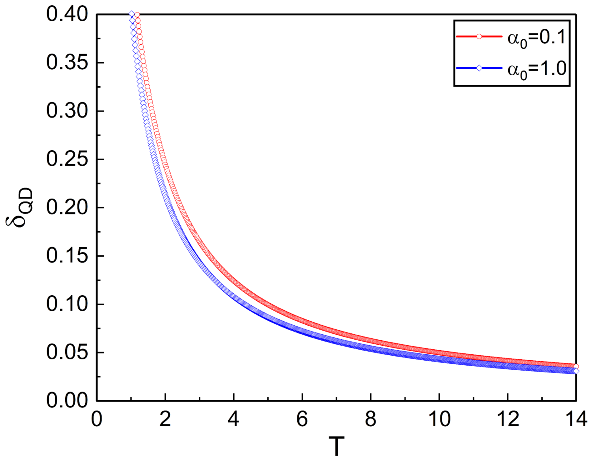
the decoherence measure is reduced to
This result is illustrated in
Figure 1 as a function of the absolute temperature.
becomes small as the temperature increases. Consequently, the quantum decoherence condition is met in the case that the temperature is sufficiently high. If the temperature gradually decreases towards absolute zero,
increases and, eventually, it reaches an extreme value (unity) in the limit
. That is,
becomes a constant at
, where this outcome agrees with the report of Kim et al., which was treated only at absolute zero temperature (see Equation (
32) in Ref. [
36]). The formula Equation (
72), which is of a particular case, also agrees with the result of Ref. [
16]. Continuous interactions of the stochastic system with the surrounding environment always result in its decoherence.
To evaluate the decoherence time, we express Equation (
35) as
where
Since the decoherence time is determined by position off-diagonal elements [
38], the conditional equation for estimating the decoherence time can be represented in the form
Thus, for the damped harmonic oscillator, the decoherence time
in position space measured from an initial time
is given by
This is the time scale required for the onset of decoherence, i.e., quantum coherence disappears exponentially on this time scale. Since a classical state is the most robust one while pure quantum states are fragile, the predictable consequences of a physical process are always classical ones. A somewhat different definition of the decoherence time is given in Refs. [
20,
37].
From the similar condition in momentum space
we have the decoherence time in momentum space for the damped harmonic oscillator:
We confirm that both Equations (
77) and (
79) do not depend on
.
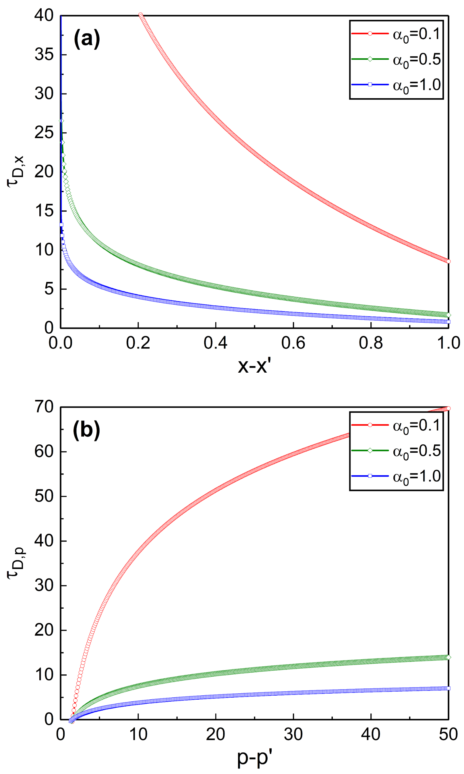
Figure 2 shows that
becomes small as
increases, whereas
becomes large as
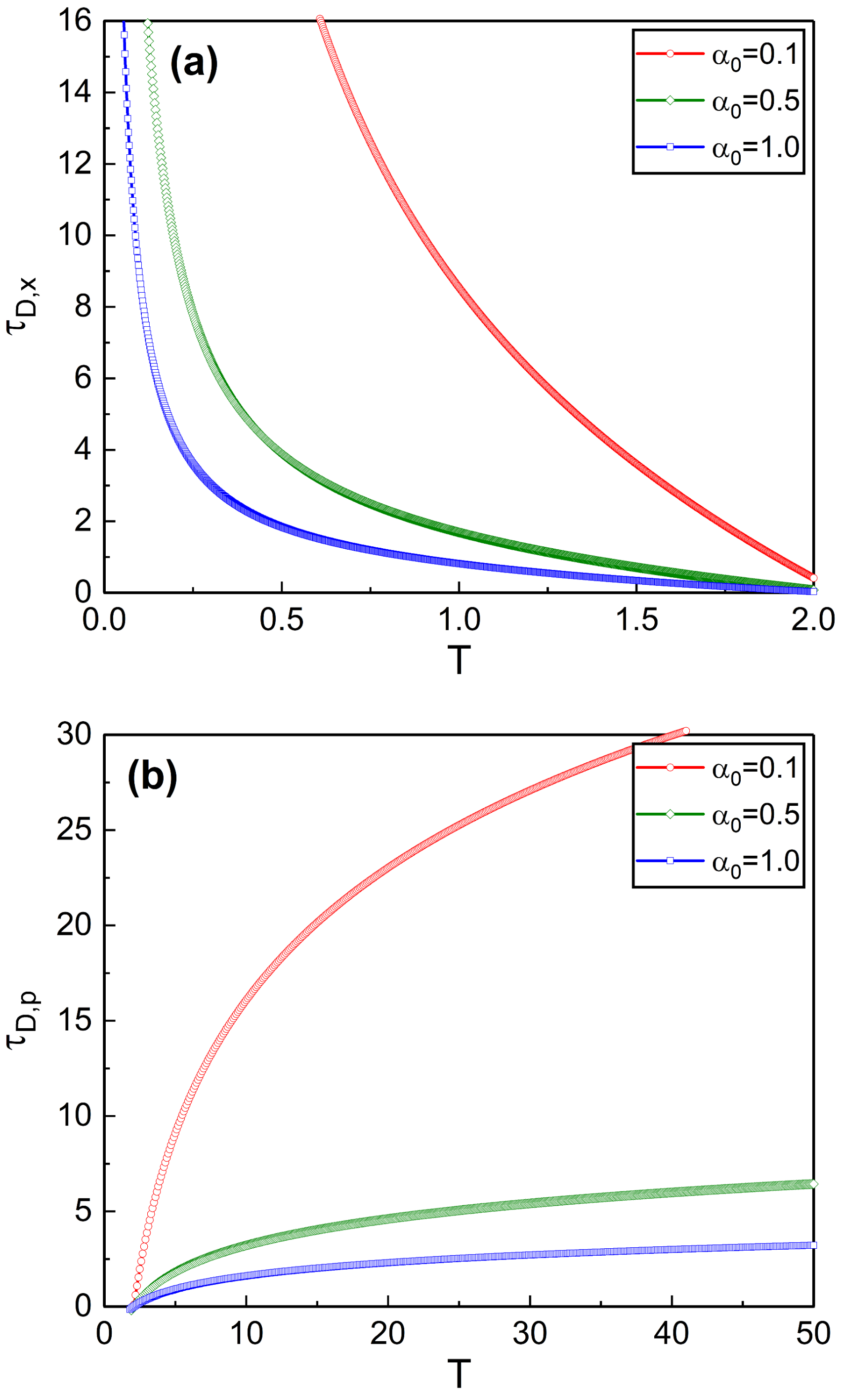
grows. We can see the effects of the increase of the absolute temperature on the decoherence time from
Figure 3.
decreases as the temperature grows while
increases in the same situation.
Now we consider the classical correlation for the damped harmonic oscillator. Using the values obtained in
Appendix C, we can represent the measure of the classical correlation given in Equation (
50) (or Equation (
64)) as
This consequence for the reduced system is correct and agrees with that of Ref. [
16]. However, it does not agree with that of Kim et al., (see Equation (
33) in Ref. [
36]), which exponentially increases with time. The classical correlation condition in our consequence is satisfied when
is sufficiently small compared to
according to Equation (
66). For the ordinary harmonic oscillator limit (
), Equation (
80) becomes infinity.
On the other hand, the measures of the absolute classical correlations in each space are given by
Notice that
exponentially increases with the lapse of time whereas
decreases exponentially. Hence, their behaviors are opposite each other in time.
The quantum coherence lengths are expressed as
Whereas
decreases exponentially with time,
increases exponentially.
is inversely proportional to
roughly, and it becomes large if
is small. This consequence is closely related to the reciprocal properties of the uncertainties of position and momentum.
5. Summary and Conclusions
Decoherence, classical correlation, and quantum coherence length of a time-varying SQS with a general environment were investigated in relation with the emergence of classicality from its initial quantum character using the invariant operator method. If we consider the arbitrariness of time dependence of the parameters, the Hamiltonian that we considered is somewhat complicated. The system dissipates with time due to not only the non-zero damping coefficient but also the time dependence of mass.
Measures for the degree of both decoherence and the classical correlation were evaluated using the wave functions. We confirmed that the classical correlation does not depend on the temperature, whereas the behavior of decoherence is different depending on the temperature. The quantum coherence lengths in position and momentum spaces vary depending on the change of parameters, but in different ways in both spaces. Quantal to classical transition of the system is affected by the time dependence of the stochastic process in this way.
For a deeper understanding of our research outcomes, we applied them to the damped harmonic oscillator. The quantum decoherence condition for that system is satisfied in the limit of high temperature. The decoherence time was estimated in both position and momentum spaces. The decoherence time in position space decreases as grows and that in momentum space increases as becomes large. Besides, the decoherence time in position space decreases as the temperature grows whereas that in momentum space increases in the same situation. The classical correlation condition is satisfied when the modified frequency of the oscillatory motion is sufficiently small compared to the damping coefficient. On the other hand, the quantum coherence length in position space decays exponentially as the damped system dissipates, whereas the momentum-space coherence length increases exponentially with time.
Although the decoherence phenomenon and the collapse of the system to a classical one have been fundamental questions in modern physics for a long time since the 1930s, the progress of related experimental techniques has now made it possible to observe and control it in laboratories [
14,
15,
42]. Many experiments in this direction have been focused on revealing how quantum systems can be robust despite the influence of an environment. For the case of our system, we considered time-variation of parameters as a generalization of the research. Hence it may be favorable to test classicality considering variation of parameters [
43,
44] in order to demonstrate our results.
The mechanism of quantum decoherence represented in the text can be applicable to many practical systems beyond stochastic systems, such as optical fibers [
45,
46], nanomechanical oscillators [
47], and evolution of the primordial universe [
48]. In particular, polarization mode dispersion in fibers induces decoherence that is detrimental in keeping the coherence of polarization entanglement. Due to this, long distance quantum communication with quantum key distribution over more than a thousand kilometers through optical fibers is one of the challenging problems.


