
Efficient Technique for Solving (3+1)-D Fourth-Order Parabolic PDEs with Time-Fractional Derivatives
 ,
,  and
and 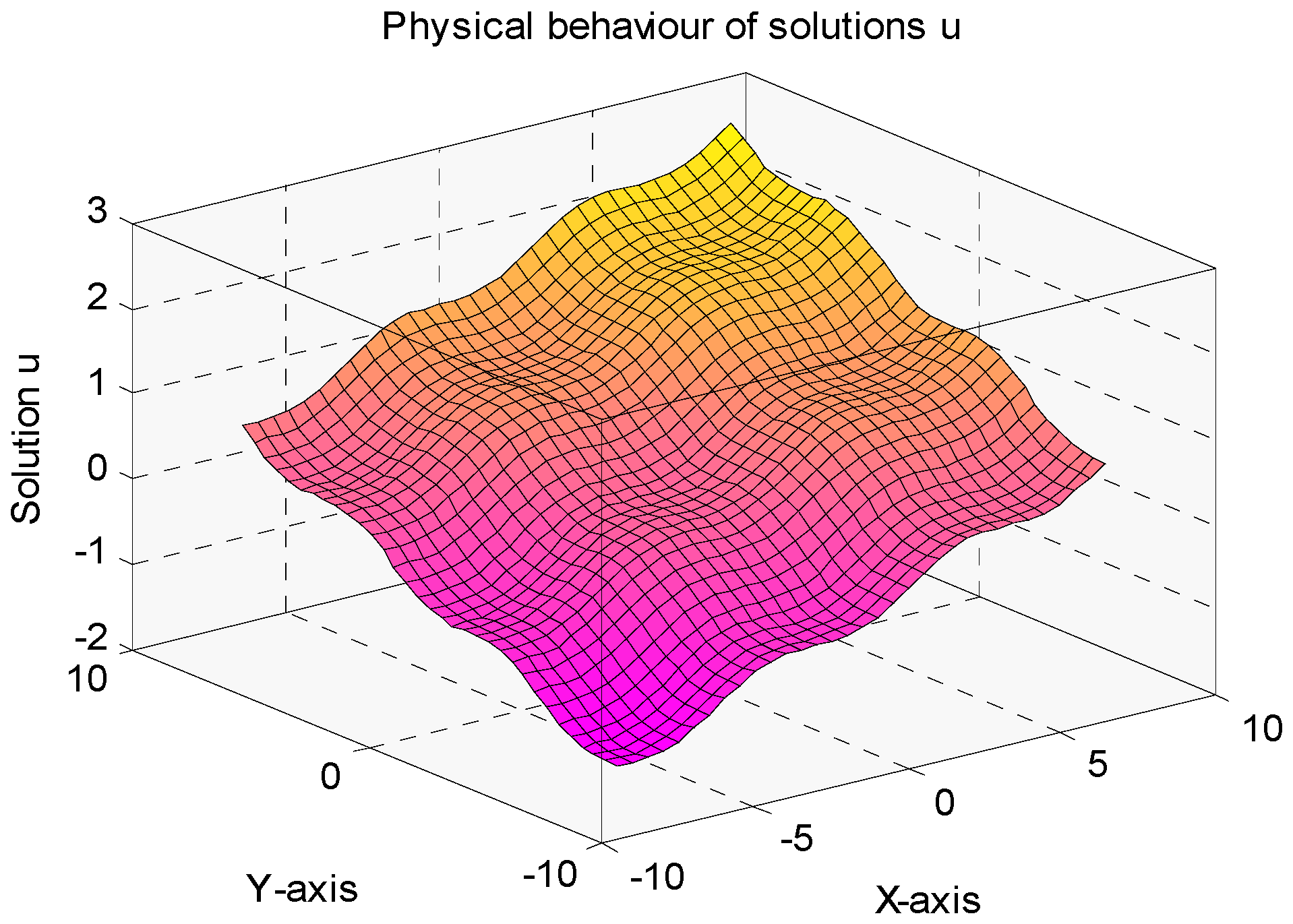
Abstract
:1. Introduction
2. Some Basic Definitions
3. Basic Properties
- The implementation of the Elzaki integral transform to the Caputo fractional derivative of the function is as follows:
- The Elzaki integral transform of some of the partial derivatives is given below:
- (a)
- (b)
- (c)
- (d)
- .
- The Elzaki transforms of some functions are listed here:
4. Classical Homotopy Perturbation Method (HPM)
5. Elzaki Transform Homotopy Perturbation Method (ETHPM)
6. Convergence Analysis
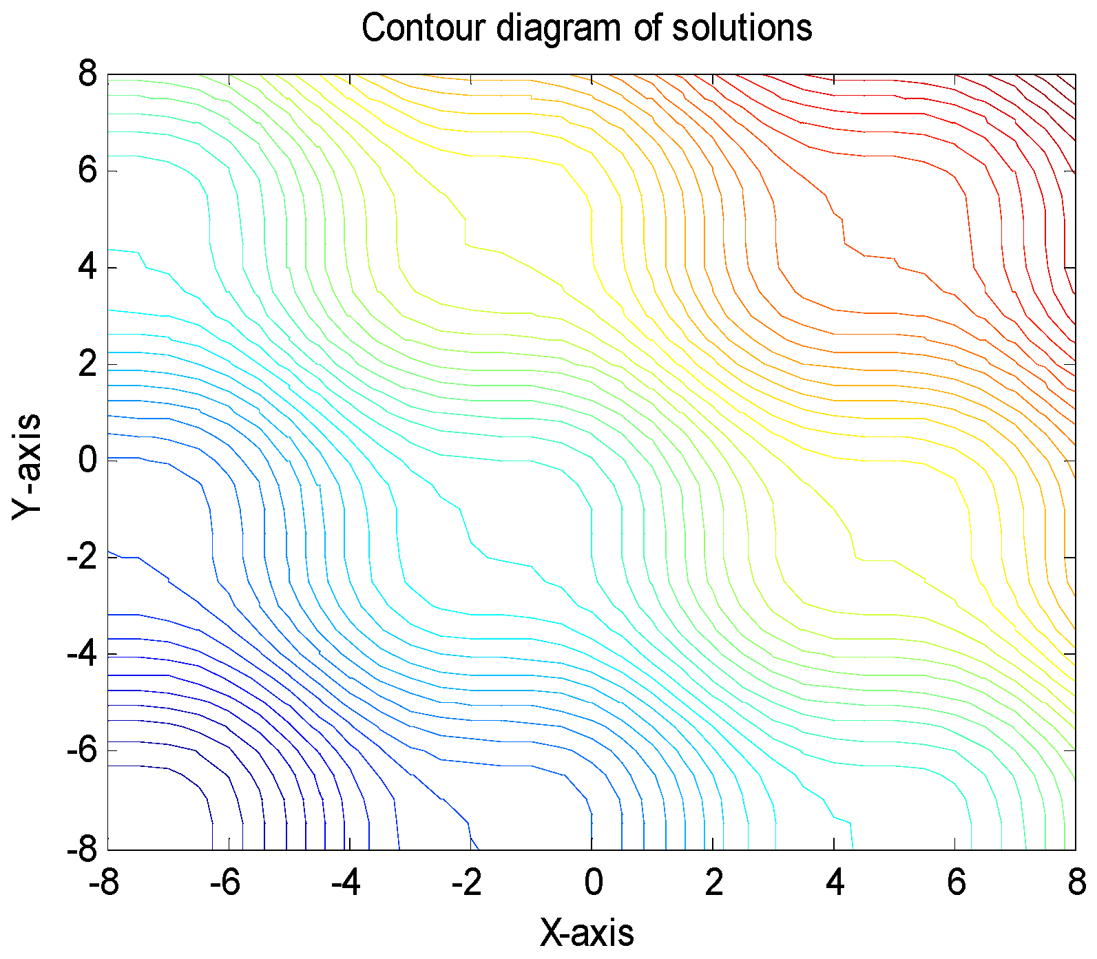
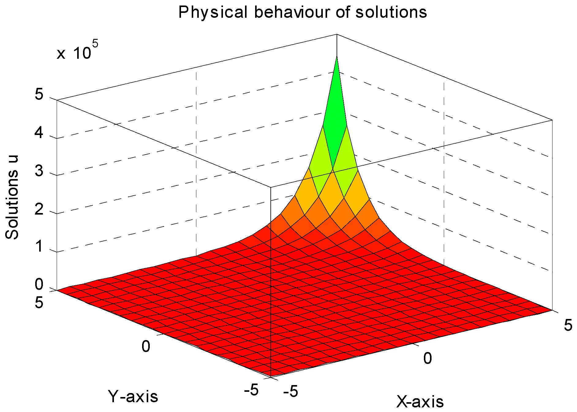
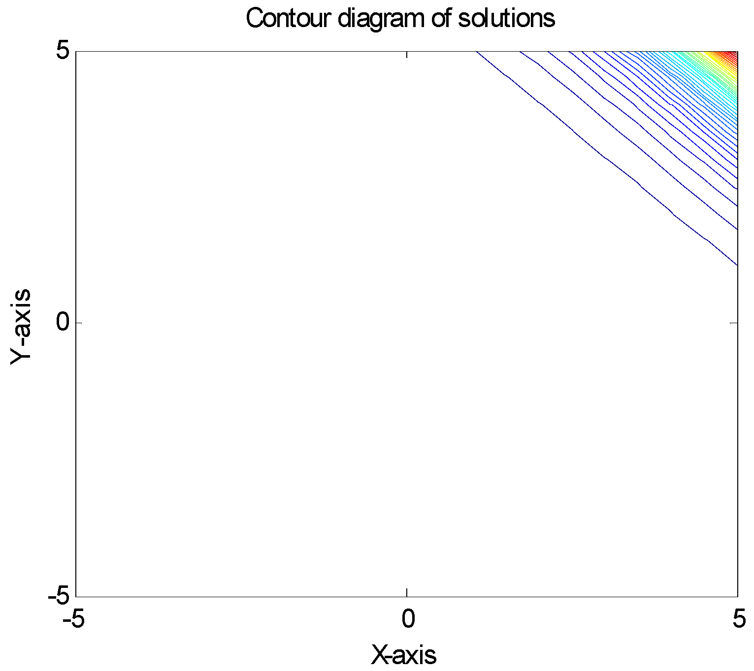
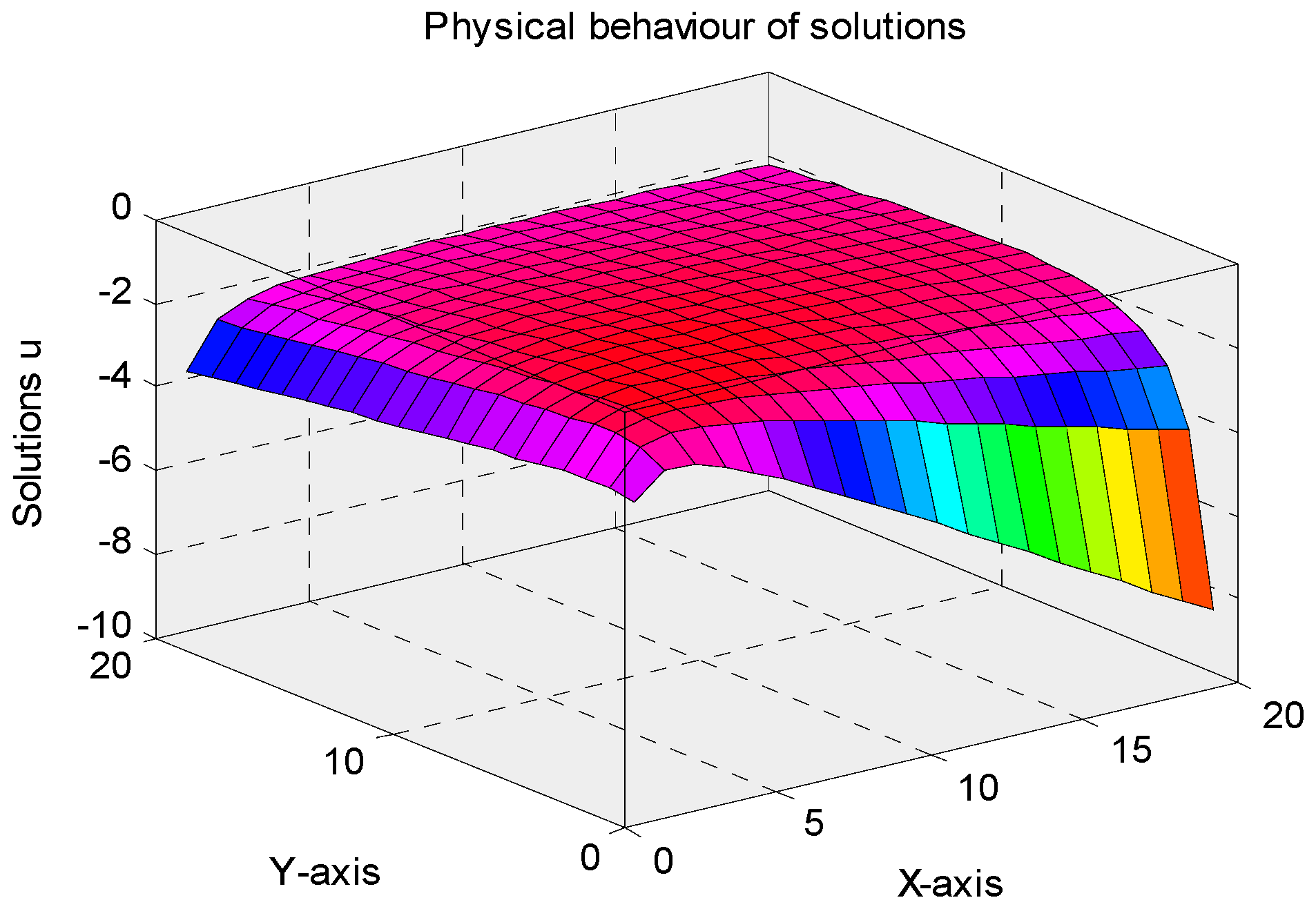
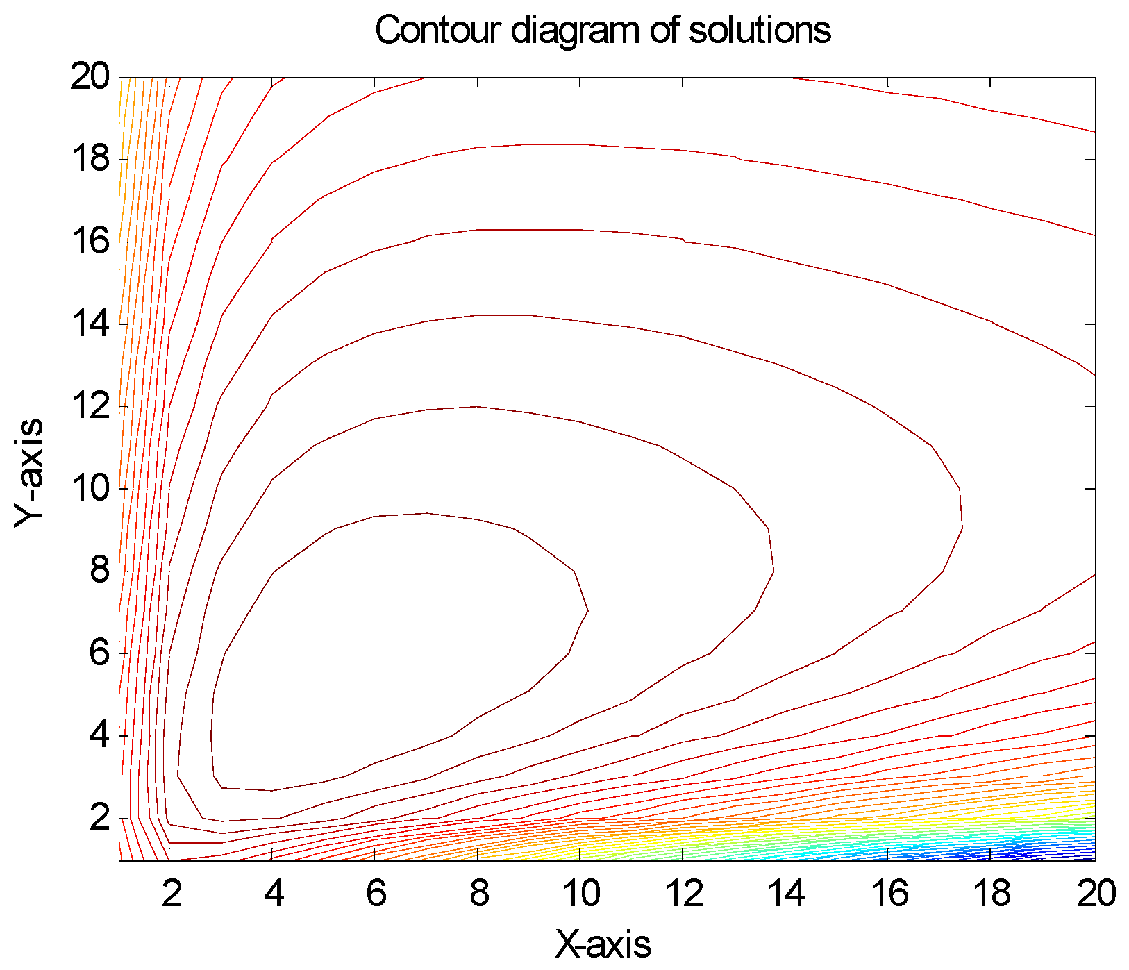
7. Numerical Experiments
8. Conclusions
Author Contributions
Funding
Data Availability Statement
Acknowledgments
Conflicts of Interest
References
- Chatibi, Y.; El Kinani, E.; Ouhadan, A. Variational calculus involving nonlocal fractional derivative with Mittag–Leffler kernel. Chaos Solitons Fractals 2018, 118, 117–121. [Google Scholar] [CrossRef]
- Podlubny, I. Fractional Differential Equations; Academic Press: San Diego, CA, USA, 1999. [Google Scholar]
- Tayyan, A.; Sakka, A.H. Lie symmetry analysis of some conformable fractional partial differential equations. Arab. J. Math. 2020, 9, 201–212. [Google Scholar] [CrossRef] [Green Version]
- Chatibi, Y.; El Kinani, E.H.; Ouhadan, A. Lie symmetry analysis of conformable differential equations. AIMS Math. 2019, 4, 1133–1144. [Google Scholar] [CrossRef]
- Baleanu, D.; Machado, J.A.T.; Luo, A.C.J. Fractional Dynamics and Control; Springer Science & Business Media: New York, NY, USA, 2011. [Google Scholar]
- Das, S. Analytical solution of a fractional diffusion equation by variational iteration method. Comput. Math. Appl. 2008, 57, 483–487. [Google Scholar] [CrossRef] [Green Version]
- Elsaid, A. The variational iteration method for solving Riesz fractional partial differential equations. Comput. Math. Appl. 2010, 60, 1940–1947. [Google Scholar] [CrossRef] [Green Version]
- Chatibi, Y.; El Kinani, E.H.; Ouhadan, A. On the discrete symmetry analysis of some classical and fractional differential equations. Math. Methods Appl. Sci. 2019, 44, 2868–2878. [Google Scholar] [CrossRef]
- Chatibi, Y.; El Kinani, E.H.; Ouhadan, A. Lie symmetry analysis and conservation laws for the time fractional Black–Scholes equation. Int. J. Geom. Methods Mod. Phys. 2019, 17, 2050010. [Google Scholar] [CrossRef]
- He, J.-H. Homotopy perturbation method: A new nonlinear analytical technique. Appl. Math. Comput. 2003, 135, 73–79. [Google Scholar] [CrossRef]
- He, J.-H. Application of homotopy perturbation method to nonlinear wave equations. Chaos Solitons Fractals 2005, 26, 695–700. [Google Scholar] [CrossRef]
- He, J.-H. Homotopy perturbation technique. Comput. Methods Appl. Mech. Eng. 1999, 178, 257–262. [Google Scholar] [CrossRef]
- He, J.-H. Some applications of nonlinear fractional differential equations and their approximations. Bull. Sci. Technol. Soc. 1999, 15, 86–90. [Google Scholar]
- He, J.-H. A coupling method of a homotopy technique and a perturbation technique for non-linear problems. Int. J. Non-linear Mech. 2000, 35, 37–43. [Google Scholar] [CrossRef]
- Tchier, F.; Inc, M.; Yusuf, A. Symmetry analysis, exact solutions and numerical approximations for the space-time Carleman equation in nonlinear dynamical systems. Eur. Phys. J. Plus 2019, 134, 1–18. [Google Scholar] [CrossRef]
- Yusuf, A.; Inc, M.; Bayram, M. Soliton solutions for Kudryashov-Sinelshchikov equation. Sigma J. Eng. Nat. Sci. 2019, 37, 439–444. [Google Scholar]
- Inc, M.; Yusuf, A.; Aliyu, A.I. Dark and singular optical Solitons for the conformable space time nonlinear Schrodinger equation with Kerr and power law nonlinearity. Optik 2018, 162, 65–75. [Google Scholar] [CrossRef]
- Inc, M.; Yusuf, A.; Aliyu, A.I. Lie symmetry analysis and explicit solutions for the time generalized Burgers-Huxley equation. Opt. Quantum Electron. 2018, 50, 94. [Google Scholar] [CrossRef]
- Elzaki, T.M. The new integral transform “Elzaki Transform”. Glob. J. Pure Appl. Math. 2011, 1, 57–64. [Google Scholar]
- Elzaki, T.M.; Elzaki, S.M. Application of new transform “Elzaki Transform” to partial differential equations. Glob. J. Pure Appl. Math. 2011, 1, 65–70. [Google Scholar]
- Elzaki, T.M.; Elzaki, S.M. On the connections between Laplace and Elzaki transforms. Adv. Theor. Appl. Math. 2011, 6, 1–11. [Google Scholar]
- Singh, P.; Sharma, D. On the problem of convergence of series solution of non-linear fractional partial differential equation. AIP Conf. Proc. 2017, 1860, 020027. [Google Scholar]
- Elzaki, T.M.; Elzaki, S.M.; Hilal, E.M.A. Elzaki and Sumudu transforms for solving some differential equations. Glob. J. Pure Appl. Math. 2012, 8, 167–173. [Google Scholar]
- Singh, P.; Sharma, D. Convergence and Error Analysis of Series Solution of Nonlinear Partial Differential Equation. Nonlinear Eng. 2018, 7, 303–308. [Google Scholar] [CrossRef]
- Singh, I. Wavelet based method for solving generalized Burgers type equations. Int. J. Comput. Mater. Sci. Eng. 2009, 8, 1950020. [Google Scholar]
- Singh, I.; Kumar, S. Haar wavelet collocation method for solving nonlinear Kuramoto–Sivashinsky equation. Ital. J. Pure Appl. Math. 2018, 39, 373–384. [Google Scholar]
- Singh, I.; Kumar, S. Haar wavelet method for some nonlinear Volterra integral equations of the first kind. J. Comput. Appl. Math. 2016, 292, 541–552. [Google Scholar] [CrossRef]
- Akgül, A. A novel method for a fractional derivative with non-local and non-singular kernel. Chaos, Solitons Fractals 2018, 114, 478–482. [Google Scholar] [CrossRef]
- Sakar, M.G.; Saldır, O.; Akgül, A. A Novel Technique for Fractional Bagley–Torvik Equation. Proc. Natl. Acad. Sci. India Sect. A Phys. Sci. 2018, 89, 539–545. [Google Scholar] [CrossRef]
- Modanli, M.; Akgül, A. Numerical solution of fractional telegraph differential equations by theta-method. Eur. Phys. J. Spec. Top. 2017, 226, 3693–3703. [Google Scholar] [CrossRef]
- Akgül, E.K.; Orcan, B.; Akgül, A. Solving Higher-Order Fractional Differential Equations by Reproducing Kernel Hilbert Space Method. J. Adv. Phys. 2018, 7, 98–102. [Google Scholar] [CrossRef]
- Mussa, Y.O.; Gizwaw, A.K.; Negassa, A.D. Three-dimensional fourth order time fractional parabolic partial differential equations and their analytical solution. Math. Probl. Eng. 2021, 2021, 1–12. [Google Scholar] [CrossRef]
- Myers, T.; Charpin, J. A mathematical model for atmospheric ice accretion and water flow on a cold surface. Int. J. Heat Mass Transf. 2004, 47, 5483–5500. [Google Scholar] [CrossRef]
- Myers, T.G.; Charpin, J.P.F.; Chapman, S.J. The flow and solidification of a thin fluid film on an arbitrary three-dimensional surface. Phys. Fluids 2002, 14, 2788–2803. [Google Scholar] [CrossRef] [Green Version]
- Halpern, D.; Jensen, O.E.; Grotberg, J.B. A theoretical study of surfactant and liquid delivery into the lung. J. Appl. Physiol. 1998, 85, 333–352. [Google Scholar] [CrossRef] [Green Version]
- Mémoli, F.; Sapiro, G.; Thompson, P. Implicit brain imaging. Neuroimage 2004, 23, S179–S188. [Google Scholar] [CrossRef] [PubMed]
- Toga, A. Brain Warping; Academic Press: New York, NY, USA, 1998. [Google Scholar]
- Hofer, M.; Pottmann, H. Energy-minimizing splines in manifolds. ACM Trans. Graph. 2004, 284–293. [Google Scholar] [CrossRef] [Green Version]
- Sharma, K.; Kumar, R.; Kakkar, M.K.; Ghangas, S. Three dimensional waves propagation in thermo-viscoelastic medium with two temperature and void. IOP Conf. Series: Mater. Sci. Eng. 2021, 1033, 012059. [Google Scholar] [CrossRef]
- Singh, V.; Saluja, N.; Singh, C.; Malhotra, R. Computational and Experimental study of microwave processing of susceptor with multiple topologies of launcher waveguide. AIP Conf. Proc. 2022, 2357, 040019. [Google Scholar]


Disclaimer/Publisher’s Note: The statements, opinions and data contained in all publications are solely those of the individual author(s) and contributor(s) and not of MDPI and/or the editor(s). MDPI and/or the editor(s) disclaim responsibility for any injury to people or property resulting from any ideas, methods, instructions or products referred to in the content. |
© 2023 by the authors. Licensee MDPI, Basel, Switzerland. This article is an open access article distributed under the terms and conditions of the Creative Commons Attribution (CC BY) license (https://creativecommons.org/licenses/by/4.0/).
Share and Cite
ZeinEldin, R.A.; Singh, I.; Singh, G.; Elgarhy, M.; Khalifa, H.A.E.-W. Efficient Technique for Solving (3+1)-D Fourth-Order Parabolic PDEs with Time-Fractional Derivatives. Axioms 2023, 12, 347. https://doi.org/10.3390/axioms12040347
ZeinEldin RA, Singh I, Singh G, Elgarhy M, Khalifa HAE-W. Efficient Technique for Solving (3+1)-D Fourth-Order Parabolic PDEs with Time-Fractional Derivatives. Axioms. 2023; 12(4):347. https://doi.org/10.3390/axioms12040347
Chicago/Turabian StyleZeinEldin, Ramadan A., Inderdeep Singh, Gurpreet Singh, Mohammed Elgarhy, and Hamiden Abd EI-Wahed Khalifa. 2023. "Efficient Technique for Solving (3+1)-D Fourth-Order Parabolic PDEs with Time-Fractional Derivatives" Axioms 12, no. 4: 347. https://doi.org/10.3390/axioms12040347