Interpreting Infinite Numbers

Abstract

The mathematical concept of infinity, in the sense of Cantor, is rather far from applied mathematics and statistics. These fields can be linked. We comment on the properties of infinite numbers and relate them to some operations with random variables. The existence of statistical parametric models can be studied in terms of cardinal numbers. Some probabilistic interpretations of Gödel’s theorem, Turing’s halting problem, and the Banach-Tarski paradox are commented upon, as well as the axiom of choice and the continuum hypothesis. We use a basic but sufficient mathematical level.

1. Introduction

The concept of infinite quantity is very old, and is often considered as a negative sentence. Though it has been around for a long time, the notion of infinite quantity is still often viewed negatively. In addition, limitless power and perfection were connected with the divine.

The distinction between finite and infinite started in ancient Greece. Zenon denied the infinity through paradoxes. Aristotle considered the infinity as something potential, never actual, an approach accepted for a long time (Gauss said that infinity was only a façon de parler). The infinity, as a number or object, was unaccepted, as it does not exist. Thomas d’Aquino in Summa Theologica, and Galileo Galilei in Discursi e demostrazione matematische, also denied the infinity. The night darkness goes against the paradox of Kepler-Olbers on the possible infinite sky. In contrast, Agustin de Hipona and Spinoza (Ethica) used the idea of the absolutely infinite.

Fontenelle in Eléments de la Géométrie de l’infini (published in 1727) refers to the infinity as an actual object, which can be operated algebraically. Bolzano in Paradoxien des Unenlidchen (published in 1854) studied some paradoxes on the infinity and defended the concept of actual infinity. The mathematical infinity was an academic leivmotiv; for instance, the discussion of Domenech y Estapa [1] on geometrical absurdities engendered by the interpretation of the mathematical infinity. He does not agree to define the straight line as a limit of a circumference whose diameter increases (so Nicholas of Cusa illustrated the meaning of infinity), as this definition may identify the extremes, i.e., the positive and the negative infinities.

The rigorous mathematical definition and study of infinite quantities starts with Georg Cantor. Galileo’s argument against the infinity, since if accepted, then natural and even numbers have the same size, was used by Cantor to define the infinite cardinality of a set. In fact, Gregory of Rimini (about 1350) had advanced that a subpart of something infinite could be equivalent to the whole.

Cantor found, compared, and operated infinities of different sizes, and despite Kronecker’s and Poincaré’s opposition, he imposed his theory and founded the so-called Transfinite Arithmetic, today accepted everywhere. It was even suggested by the academic Rodriguez-Salinas [2] that Homo Sapiens, after Cantor, should be Homo Trans-Sapiens.

This article deals with the following related concepts:

• The infinite cardinality (size) of sets.
• Operating random variables and transfinite arithmetic.
• Gödel’s theorem and parametric statistics.
• The cardinality of some bivariate distributions.
• The axiom of choice and the continuum hypothesis.
• The probabilistic analogy of the Banach-Tarski theorem.

Statistics is a very wide subject, and most statisticians do not know some topics on infinite cardinals. The aim of this article is to show, in a basic way, these concepts, and to establish a parallelism between transfinite arithmetic and some operations with random variables, as well as the dimensionality of statistical models and other concepts in the field of statistics and probability.

For a rigorous and coherent introduction to the set theory, see [3]. For a history of the concept of infinity, see chapter 2 in [4]. See [5,6] for a description of the infinities of different sizes. The biography and contributions of Cantor are well explained in [7].

2. Essentials on Cardinals and Transfinite Arithmetic

Any non-empty set $\mathbb{A}$ has a cardinal number denoted $\#\mathbb{A}$. If the elements of $\mathbb{A}$ are in one-to-one correspondence with the elements of a proper subset of $\mathbb{A}$, then the cardinal $\#\mathbb{A}$ is infinite.

Accordingly, we can give the cardinal number #$Ø=0$ to the empty set, as well as $\#\{a_1,\dots ,a_k\}=k$ if k is a natural number and $a_i\ne a_j$ for $i\ne j$. The most interesting infinite cardinals are $\#\mathbb{N}$ and $\#\mathbb{R}$, where $\mathbb{N}=\{0,1,\dots ,n,\dots \}$ is the infinite countable set—called denumerable—of the natural numbers, and $\mathbb{R}$ is the uncountable set of the real numbers. The notations for these infinite cardinals are:

$$\#\mathbb{N}={\aleph }_0,\#\mathbb{R}=\mathbf{c}.$$

The infinite cardinal $\mathbf{c}$ is the power of the continuum. It is well known in set theory that

$${\aleph }_0<\mathbf{c}=2^{{\aleph }_0}=\#\mathcal{P}\left(\mathbb{N}\right),$$

where $\mathcal{P}\left(\mathbb{N}\right)$ is the family of all subsets of $\mathbb{N}$.

The inequality $\#\mathbb{N}<\#\mathcal{P}\left(\mathbb{N}\right)$ is a particular case of Cantor’s theorem: Any non-empty set $\mathbb{A}$ satisfies $\#\mathbb{A}<$$\#\mathcal{P}\left(\mathbb{A}\right)$ [3].

If ↔ stands for the one-to-one correspondence between two sets, then the equality, inclusion, and two elementary operations with cardinals are:

$$\begin{array}{lll}\mathrm{Equality}\hfill & \#\mathbb{A}=\#\mathbb{B}& \mathrm{if}\mathbb{A}\leftrightarrow \mathbb{B}\hfill \\ \mathrm{Inequality}\hfill & \#\mathbb{A}\le \#\mathbb{B}& \mathrm{if}\mathbb{A}\subseteq \mathbb{B}\hfill \\ \mathrm{Sum}\hfill & \#\mathbb{A}+\#\mathbb{B}=\#(\mathbb{A}\cup \mathbb{B})& \mathrm{if}\mathbb{A}\cap \mathbb{B}=Ø\hfill \\ \mathrm{Product}\hfill & \#\mathbb{A}\times \#\mathbb{B}=\#(\mathbb{A}\times \mathbb{B})& \mathrm{if}\mathbb{A},\mathbb{B}\mathrm{are}\mathrm{general}\mathrm{sets}.\hfill \end{array}$$

For instance, $\mathbb{N}\leftrightarrow \mathbb{Q},$ where $\mathbb{Q}$ is the set of rational numbers, so $\mathbb{Q}$ is infinite countable.

In transfinite or cardinal arithmetic, the following rules hold, where n is any finite natural number:

$$\begin{array}{cc}\hfill n+{\aleph }_0& ={\aleph }_0,{\aleph }_0+{\aleph }_0={\aleph }_0,\hfill \\ \hfill {\aleph }_0\times {\aleph }_0& ={\aleph }_0,{\aleph }_0+\mathbf{c}=\mathbf{c},\hfill \\ \hfill \mathbf{c}+\mathbf{c}& =\mathbf{c},\mathbf{c}\times \mathbf{c}=\mathbf{c}.\hfill \end{array}$$

Thus, $\#\mathbb{R}=\#{\mathbb{R}}^2=\#{\mathbb{R}}^3=\mathbf{c}.$ Hence, the real line, the Euclidean plane, and the three-dimensional space have the same uncountable cardinality $\mathbf{c}$, the power of the continuum.

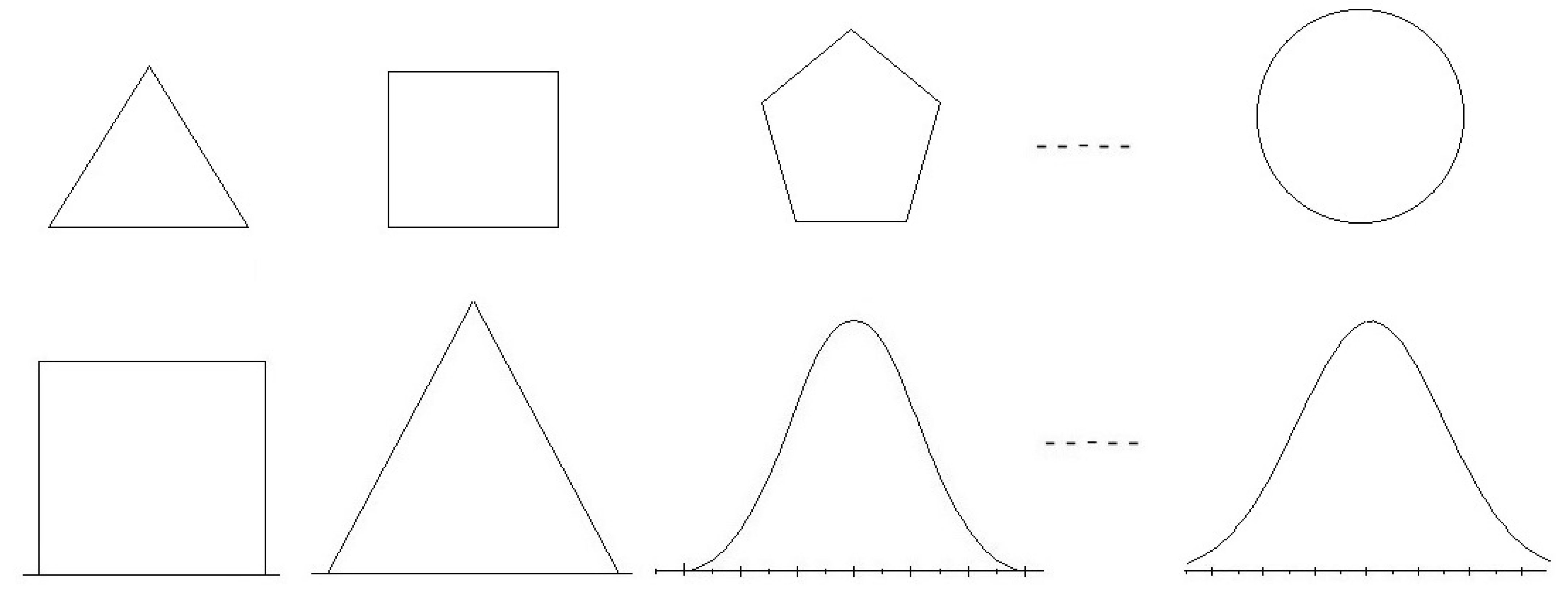
If we consider a regular polygon ${\mathbb{V}}_n$ with n vertices, circumscribed in a circumference, the limit, as n increases, is ${\mathbb{V}}_{\infty },$ the circumference with infinite countable points. Although ${\aleph }_0<\mathbf{c}$, it is impossible to distinguish geometrically between ${\mathbb{V}}_{\infty }$ (cardinality ${\aleph }_0$) and the complete continuous circumference (cardinality $\mathbf{c}$); see Appendix A. The central limit theorem also illustrates the meaning of infinity. Both examples (geometric and probabilistic) are depicted in Figure 1. Another paradigm, described by Nicholas of Cusa (about 1445), of the infinite cardinality $\mathbf{c}$ is the straight line, thought of as the limit of a circle whose diameter increases constantly.

3. Operating Poisson and Gaussian Distributions

Let us indicate Poisson$\left(n\right)$, the Poisson random variable with parameter n (both the expectation and variance are n), where n is fixed and n $\in \mathbb{N}.$ If Poisson${\left(m\right)}_1$ and Poisson${\left(n\right)}_2$ are independent, then the sum of both variables is also Poisson$(m+n).$

When n is ranging in $\mathbb{N}$, this family of discrete random variables is indicated by [Poisson$\left(n\right)$].

Similarly, if Normal$(\mu ,{\sigma }^2)$ is the normal random variable with mean $\mu$ and variance ${\sigma }^2,$ then [Normal] is the family of all normal random variables. The sum of independent normal variables is also normal. Accordingly, the bivariate normal family can be indicated by [Normal, Normal], and all continuous univariate and bivariate variables are indicated by [All r.v.] and [All r.v., All r.v.], respectively.

It is clear that $\#[$Poisson$\left(n\right)] =$${\aleph }_0$ and $\#[$Normal$] =$$\mathbf{c}.$ As [All r.v.] is described by the all positive curves (continuous or not continuous) with area 1, and it is well-known that the cardinality of this family is #[All]$=2^{\mathbf{c}}=\#\mathcal{P}\left(\mathbb{R}\right).$ In addition, if [Poisson$\left(n\right)$]${}_1$ and [Poisson$\left(n\right)$]${}_2$ are independent, as each variable is an application from the sample population to $\mathbb{N}$, and we can interpret that there are no common variables, so (ignoring the constant 0) the intersection of both sets is empty. By $\mathbb{Q} +$[Normal], we indicate all the possible sums $q + X,$ where q is rational and X is random normal.

With these notations, since ${\aleph }_0=\#\mathbb{Q},$${\aleph }_0=\#$[Poisson(n)], $\mathbf{c}=\#$[Normal], etc., we have a relation between some operations with random variables and cardinal numbers; see

Table 1. Relatiing some operations with cardinals and random variables.

Random Variables	Cardinals
[Poisson$\left(n\right)$]${}_1 +$ [Poisson$\left(n\right)$]${}_2=$ [Poisson$\left(n\right)$]	${\aleph }_0+{\aleph }_0={\aleph }_0$
$\mathbb{Q} +$ [Normal] = [Normal]	${\aleph }_0+\mathbf{c}=\mathbf{c}$
[Normal]${}_1$ + [Normal]${}_2$ = [Normal]	$\mathbf{c}+\mathbf{c}=\mathbf{c}$
[Normal] + [All r.v.] = [All r.v.]	$\mathbf{c}+2^{\mathbf{c}}=2^{\mathbf{c}}$
[Normal, Normal] = [Bivariate normal]	$\mathbf{c}\times \mathbf{c}=\mathbf{c}$
[All r.v., All r.v.] = [Bivariate all]	$2^{\mathbf{c}}\times 2^{\mathbf{c}}=2^{\mathbf{c}}$

.

4. Gödel’s Theorem

Bolzano had proven that the number of mathematical propositions is infinite. Gödel proved that there are also infinite propositions on the integer numbers, which cannot be reduced to a finite number of axioms. This is a special case of the famous theorem enunciated by Kurt Gödel in 1931. This theorem says that in a logical system based on axioms and containing the Arithmetic, we have some propositions which cannot be proven. These propositions are undecidable: they can be accepted or rejected. The acceptance should be considered as a new axiom. An example is the fifth postulate of Euclides on parallel lines, which cannot be proven as a consequence of the other four axioms. Another example is the hypothesis of the continuum (see below), posed by Cantor: there does not exist a set $\mathbb{G}$ with cardinality $\mathbf{g}$ between the infinite countable (denumerable) and the uncountable; i.e., it is not possible to find $\mathbf{g}$ such that ${\aleph }_0<\mathbf{g}<\mathbf{c}.$ However, this hypothesis can be accepted or rejected, without prejudice to the Arithmetic.

Let us understand Gödel’s theorem with a broad view, and interpret this theorem from a statistical perspective, namely, in terms of observable events, parametric models, inference, etc. A statistical model is a family of probability distributions parametrized by a parameter $\theta .$ The Poisson distribution with parameter $\lambda$ and the normal distribution with parameters $\mu ,$${\sigma }^2,$ are two examples, with a parameter space of dimensions one and two, respectively. If $F_{\theta }$ is a statistical model, with $\theta$ belonging to a region of ${\mathbb{R}}^k,$ with positive hypervolume, then clearly, $\#F_{\theta }=\mathbf{c}.$

Question: Does there exist a universal parametrization covering all distributions? The answer is no. Let us consider all probability distributions with the same support. This set has cardinal $2^{\mathbf{c}}.$ If we suppose all of the models described by $F_{\theta },$ since $\#F_{\theta }=\mathbf{c}<2^{\mathbf{c}},$ there are many distributions out of this family. Thus, a parametrization can not cover all distributions. See an analytic proof in Appendix A.

As well, as a logical system is incomplete, since some propositions are undecidable, a statistical model, as wide as possible, is also incomplete, since some probability distributions are not contained in the model. This justifies the so-called non-parametric statistics, an approach that makes inferences on functional expressions, considering the whole set of distributions, but avoiding the use of parameters.

Another analogy is as follows. Given a sample of size $n,$ to perform an inference on the mean $\mu$ in the normal model $N(\mu ,{\sigma }_0^2),$ with the variance ${\sigma }_0^2$ being known, the statistic $\sum x_i$ is sufficient and complete. However, $\sum x_i$ is not sufficient and complete to perform an inference on $N(\mu ,{\sigma }^2),$ where both parameters are unknown. We need two statistics, namely $\sum x_i$ and $\sum x_i^2.$

Similarly, let us consider the Poisson distribution whose support is $\mathbb{N}.$ Theoretically, we can observe any subset of $\mathbb{N}$. However, $\#\mathcal{P}\left(\mathbb{N}\right)=\mathbf{c},$ and the cardinality is too large. Thus, some events can be observed, e.g., “a value k is even number”, but many other events cannot be enunciated using our limited language; hence, these events cannot be observed.

5. Turing’s Halting Problem

This problem was posed by Allan Turing in 1935. There is no general algorithm that is capable of determining whether or not a computer program will finish running. This is another example of an undecidable proposition in Gödel’s sense. From a statistical perspective, Chaitin’s approach [8] is quite interesting. A summary is next given.

Let us consider the Cantor space of all binary infinite sequences. A computer program is a subset of this space. Let P be the set of halting programs. If p is a halting program of $\left|p\right|$ bits, the probability that a randomly chosen binary sequence of length $\left|p\right|$ coincides with p is $2^{-\left|p\right|},$ provided that we generate this sequence of $0s$ and $1s$ independently with the same probability $1/2.$ In general, when choosing a program at random, the probability of achieving a halting program is

$$\Omega =\sum _{p\in P}{2}^{-\left|p\right|}.$$

That is, $\Omega ={\sum }_n{a}_n/2^n,$ where $a_n$ is the number of halting programs of n bits, taking into account that if the program with sequence $\mathbf{b}=b_1\cdots b_{n-1}$ of $(n-1)$ bits halts, then the $a_n$ programs of n bits cannot begin with $\mathbf{b}.$ This constrains $a_n.$

If $\Omega =0$, no program halts. If $\Omega =0.16$, then there is $16\%$ halt. If $\Omega =1$, all programs halt. However, $\Omega$ is not fixed, but is random. We need an algorithm of n bits to determine the first $n$ bits of $\Omega .$ This probability behaves as if it were randomly generated, just as explained above. There is not a law reducing the computation of $\Omega .$ None, some, or all programs finish running. Consequently, the halting problem is undecidable.

A short, informal proof of the halting problem, based on cardinal comparison, is given in Appendix A.

6. Cardinality of Bivariate Distributions

A bivariate cumulative distribution function $H(x,y)$ of two random variables $X,$$Y,$ with univariate marginal distributions $F\left(x\right),$$G\left(y\right),$ is usually described by a parametric model. Suppose that the range of the variables $X,$ Y are the intervals $[a,b],$$[c,d].$ If the degree of dependence between the random variables is quantified by means of a unique parameter, the cardinality of H is 1. However, in general, H admits the canonical decomposition

$$dH(x,y)=dF\left(x\right)dG\left(y\right)\left[1+\sum _{n\ge 1}{\rho }_n{a}_n\left(x\right)b_n\left(y\right)\right],$$

where ${\rho }_n$ are the canonical correlations, all positive, and $a_n\left(x\right),$ $b_n\left(y\right)$ are the canonical functions. Then, the cardinality of $H(x,y)$ is $\#\left\{{\rho }_n\right\},$ the power of the set of canonical correlations. This number, also called rank of H, is the dimensionality from a geometrical point of view, related to the so-called chi-squared distance between two observations $x.$$x^{\prime }$ of the variable $X,$

$${\delta }^2(x,x^{\prime })={\int }_c^d{\left[{\displaystyle \frac{dH(x,y)}{dF\left(x\right)dG\left(y\right)}}-{\displaystyle \frac{dH(x^{\prime },y)}{dF\left(x^{\prime }\right)dG\left(y\right)}}\right]}^{2}dG\left(y\right).$$

See [9] for a continuous correspondence analysis interpretation. Some (finite and infinite) cardinalities of $H(x,y)$ are reported in

Table 2. Cardinality of some bivariate distributions, defined as the size of the set of canonical correlations. Note the power of the continuum cardinality of the last distribution.

Bivariate Distributions Where $\mathit{F}\left(\mathit{x}\right),\mathit{G}\left(\mathit{y}\right)$ Are Indicated by $\mathit{F},$ G	Cardinality
$FG$ (stochastic independence)	0
$FG[1+\theta (1-F\left)\right(1-G\left)\right]$	1
$FG+{\theta }_1(F-F^2)(G-G^2)+{\theta }_2(2F^2-F)(1-F)(2G^2-G)(1-G)$	2
$FG/[1-\theta (1-F\left)\right(1-G\left)\right]$	${\aleph }_0$
$min{\{F,G\}}^{\theta }{\left(FG\right)}^{1-\theta }$	$\mathbf{c}$

.

In all cases, we can consider $0\le \theta \le 1.$ Thus, $H(x,y)=F\left(x\right)G\left(y\right),$ corresponding to the stochastic independence, the cardinality being 0 because of the absence of positive canonical correlations. The cardinality of the second model is 1 because the only canonical correlation is ${\rho }_1=\theta /3.$

Any distribution with infinite cardinality, e.g., $FG/[1-\theta (1-F\left)\right(1-G\left)\right]$, can be approximated by another one with finite cardinality [10].

It is worth noting the power of the continuum cardinality of the fifth model (see Table 2), defined and studied in [11,12]. In the uniform marginal case, $F\left(x\right)=x,$$G\left(y\right)=y,$$H(x,y)=min{\{x,y\}}^{\theta }{\left(xy\right)}^{1-\theta },$ the set of canonical correlations is the function $\theta {\rho }^{1-\theta }$, where $0\le \rho \le 1.$ This continuous function ranges between 0 and $\theta .$ Thus, if $\theta >0,$ the power of the set of canonical correlations is $\mathbf{c}=\#\left\{\theta {\rho }^{1-\theta }\right\}.$

Another continuous correlation model is $F\left(x\right)G\left(y\right)[1-\theta lnmax\{F\left(x\right),G\left(y\right)\left\}\right].$ In the uniform case with $\theta >0$, the cardinality of this distribution is $\mathbf{c}=\#\left\{\theta \rho \right\},$ which is also the power of the continuum.

These two distributions admit an integral expansion, instead of a series expansion, and the set of canonical correlations is not countable, but continuous. This transition from countable to continuous uncountable cardinality agrees with the hypothesis explained in the next section.

7. The Continuum Hypothesis

This hypothesis stated by Cantor in 1878 [13] says that there is no set with cardinality between the infinite countable ${\aleph }_0$ and the uncountable $\mathbf{c}.$ It can be expressed as

$${\aleph }_0<\mathbf{c}={\aleph }_1,$$

where ${\aleph }_1$ is the next immediate infinity after ${\aleph }_0.$ According to Cantor, ${\aleph }_1$ exists and is $\mathbf{c}.$ Nonetheless, this is considered undecidable after the results by Gödel and Cohen in 1940 and 1963, respectively. Nowadays, we should write

$${\aleph }_0<\mathbf{c}\le {\aleph }_1.$$

It is known of Cantor’s futile attempts in showing this hypothesis, which was included as an unsolved question in the list of 23 problems posed by Hilbert in 1900. Gödel showed that the acceptance of this hypothesis is not contradictory, whereas Cohen showed that it can be considered false and that it is not contradictory either. Thus, the continuum hypothesis is independent of the axioms of the Zermelo-Fraenkel theory of sets [3].

It is quite surprising that some authors [14,15,16,17], many years later, ignored this essential difficulty and mentioned this problem as interesting but not solved yet. The first widespread reference to Cohen and the independence of the continuum hypothesis appeared in a textbook in 1965 [18]. In the Spanish literature on this topic, [19,20] are the first books paying attention to the independence of this hypothesis. Many years later, this hypothesis still has interest [6,21].

Indeed, in probability and statistics, this hypothesis is implicitly accepted. In general, only the probabilities of subsets of $\mathbb{N}$ are considered under discrete models (such as the Poisson distribution). In addition, only Borel sets under continuous models (such as the Gaussian distribution), are taken into account. Recall that a Borel set is obtained by joining the isolated points and intervals of the real line. To define the probability of other sets is not considered, as they are unobservable. For example, accepting the axiom of choice (see below), we can construct non-measurable sets, it, however, being impossible after an experience to decide on the presence or absence of any of these sets. That is, given a value x of the random variable, it is impossible to decide whether or not x belongs to a non-measurable set of $\mathbb{R}.$ See Appendix A.

8. Axiom of Choice

This axiom (stated by Zermelo in 1904) postulates that given a family of non-empty sets, we can choose an element of each set and construct a new set with these elements. Two examples are as follows. If we consider all of the circumferences centered in the origin $(0,0)$, we do not need this axiom, as we can choose a point of each circumference, e.g., the point on the right cutting the horizontal axis. However, if we consider the family of all closed curves in the plane, we need the axiom of choice to choose a point of each curve.

Some properties in algebra, geometry, topology, and analysis depend on this axiom. One functional analysis application is to prove the null norm of the eigenfunctions of a kernel with respect to another kernel, with both being related to the last bivariate distribution given in Table 2 [22].

With some imagination, we can establish a comparison between this axiom (choosing an element of each set) and the Bayes theorem (the probability that an observation belongs to each set or cause).

However, accepting the axiom of choice, we can prove the existence of a mathematical object, but we are not able to actually construct that object. This may be a trouble. For instance, any vector space has a basis. However, there are vector spaces, e.g., $(\mathbb{Q},\mathbb{R}),$ such that the basis is unknown. This also happens with the vector space of all random variables with support in $\mathbb{R}$. In addition, accepting this axiom, some subsets of $\mathbb{R}$ lack length (Lebesgue measure) or probability (see the Appendix A). Another anomaly is next commented upon.

9. Banach-Tarski’s Theorem

Let us suppose that $\mathbf{B}$ is a solid ball. This theorem asserts that we can divide $\mathbf{B}$ into $m+n$ non-overlapping parts, i.e.,

$$\mathbf{B}=A_1\cup \cdots \cup A_m\cup B_1\cup \cdots \cup B_n,$$

and, after isometric transformations $A_i\to A_i^{*},$ $B_j\to B_j^{*},$ we can assemble these parts to yield two balls:

$$\mathbf{B}=A_1^{*}\cup \cdots \cup A_m^{*}\mathrm{and}\mathrm{also}\mathbf{B}=B_1^{*}\cup \cdots \cup B_n^{*}.$$

Accordingly, this may be expressed as the paradoxical equidecomposition

$$\mathbf{B}={\mathbf{B}}_1\cup {\mathbf{B}}_2\mathrm{with}{\mathbf{B}}_1\cap {\mathbf{B}}_2=Ø,$$

being that the volume is the same: $\left|\mathbf{B}\right|=\left|{\mathbf{B}}_1\right|=\left|{\mathbf{B}}_2\right|.$ Thus, the initial ball can be duplicated. Notice that the parts $A_i,$$B_j,$ are non-measurable subsets of $\mathbf{B}.$ In fact, it is necessary to accept the axiom of choice to prove this surprising result.

There is a probabilistic analogy. Suppose that X is a normal random variable with a mean of 0 and a variance of ${\sigma }^2.$ Then, we can decompose X as a sum, i.e., to express $X=X_1+X_2,$ the sum of two independent normal variables with mean $0.$ If $\left[X\right]$ stands for the class of variables $\alpha X,$ where $\alpha$ is a real parameter, and similarly $\left[X_1\right],$$\left[X_2\right],$ then

$$\left[X\right]=\left[X_1\right]+\left[X_2\right]\mathrm{with}\left[X_1\right]\cap \left[X_2\right]=0,$$

being $\left[X\right]\stackrel{sd}{=}\left[X_1\right]\stackrel{sd}{=}\left[X_2\right],$ where “$\stackrel{sd}{=}$” means “same distribution”. This is so because $\alpha X=\alpha X_1+\alpha X_2$ and $\left[X_1\right],$$\left[X_2\right]$ are independent; hence, they do not contain common variables, except for the constant $0.$ In spite of this lack of coincidence, these sets contain exactly the same family of normal distributions. Thus, in some sense, $\left[X\right]$ can be duplicated.

Of course, the sum of non-coincident sets of random variables is not the union of disjoint sets, but the analogy is clear; see

Table 3. Analogy between dividing a ball into two balls of the same volume, and decomposing a class of normal variables into the sum of two independent classes with the same size.

Banach-Tarski	Disjoint Balls	Same Volume	B Is Divided into
$\mathbf{B}={\mathbf{B}}_1\cup {\mathbf{B}}_2$	${\mathbf{B}}_1\cap {\mathbf{B}}_2=Ø$	$\left|\mathbf{B}\right|=\left|{\mathbf{B}}_1\right|=\left|{\mathbf{B}}_{2.}\right|$	Non-Measurable Parts
Normal class	No coincident	Same distributions	X is sum of r.v.’s with
$\left[X\right]=\left[X_1\right]+\left[X_2\right]$	$\left[X_1\right]\cap \left[X_2\right]=0$	$\left[X\right]\stackrel{sd}{=}\left[X_1\right]\stackrel{sd}{=}\left[X_2\right]$	unknown distribution

.

Furthermore, taking into account the central limit theorem, let us admit that X normal can be interpreted as the sum of a series of independent random variables, whose distributions are unknown. Namely, $X={\sum }_{i\ge 1}{X}_i,$ where the convergence is in law (the standardization is omitted). Then,

$$X=\sum _{i\mathrm{odd}}{X}_i+\sum _{i\mathrm{even}}{X}_i,$$

and X is the sum of two independent normal random variables. Note that “unknown distribution” would correspond to “non-measurable subset” in the above Banach-Tarski decomposition.

Finally, removing the constant $0,$ we can consider $\left[X\right],$$\left[X_1\right],$ $\left[X_2\right]$ projective spaces, so that we have another analogy in terms of projective geometry.

10. Discussion, Conclusions, and Future Work

The old pamphlet [1] is an example of how a mathematician and also architect—for a long time, the careers of Mathematics and Architecture overlapped in some universities—perceived contradictions between descriptive geometry and pure mathematics. However, most subjects of Mathematics and Statistics can be related. For instance, if $\mathbf{E}$ is the vector space generated by random variables, the dual space ${\mathbf{E}}^{*}$ can be interpreted as the population (set of individuals), since if $\omega$ is an individual and Y is a random variable, we can associate the real number $Y\left(\omega \right)$ to the pair $(\omega ,Y)$ [23]. The differential geometry can be used to define geodesic distances between the parameters of a statistical model [24,25]. The study of bivariate exchangeable distributions can be performed using functional analysis [22]. There are more examples linking different fields.

We have proven that some concepts and properties of Probability and Statistics can be useful for understanding and interpreting the main properties of the infinite cardinals.

Several proposals for future research are:

(1)

Analytic geometry. The equation $x^{2n}+y^{2n}=1$ defines a closed curve tending to a square as $n\to \infty .$ Study the implicit equation of other regular polygons (see Figure 1) in the same way.

(2)

Inference. Given a sample of size $n,$ the statistics $\sum x_i.$$\sum x_i^2$ are sufficient to perform inference on the normal model. Then, we may explore the sufficiency of $\sum x_i,$$\sum x_i^2,\cdots , \sum x_i^k$ under a perspective similar to Gödel’s theorem. That is, to study what kind of inference is “undecidable” on a specific model. Note that we can make a non-parametric inference if $k=n.$

(3)

Bivariate distributions. We have passed from distributions with countable cardinality to uncountable continuous cardinality. Does it give enough evidence for accepting the hypothesis of the continuum?

(4)

Banach-Tarski theorem. Removing the constant $0 \mathrm{and}$ interpret $\left[X\right]=\left[X_1\right]+\left[X_2\right]$ as a decomposition of projective spaces, which can be generalized to a higher dimension. In addition, for $k>2,$ study the comparison between dividing a ball into k balls and decomposing a normal random variable into the sum of k independent random variables.

(5)

Statistical models. The cardinality of the Poisson (with parameter being a natural number) and the normal models are ${\aleph }_0$ and $\mathbf{c},$ respectively. Are there parametric models with cardinalities larger than $\mathbf{c}$?

References

- Domenech y Estapa, J. Absurdos geométricos que engendran ciertas interpretaciones del infinito matemático. Mem. Real Acad. Cienc. Artes de Barcelona 1894, 1, 315–329. [Google Scholar]
- Rodriguez-Salinas, B. Verdades no demostrable: Teorema de Gödel y sus generalizaciones. In Real Academia de Ciencias. Horizontes Culturales; Espasa: Madrid, Spain, 2002; pp. 57–62. [Google Scholar]
- Schimmerling, E. A Course on Set Theory; Cambridge University Press: Cambridge, UK, 2011. [Google Scholar]
- Graham, L.; Kantor, J.-M. Naming Infinity; Harvard University Press: Cambridge, UK, 2009. [Google Scholar]
- Dauben, J.W. Georg Cantor. Investigación y Ciencia; Temas: Grandes Matemáticos, Spain, 1995; pp. 94–105. [Google Scholar]
- Delahaye, J.-P. Demostrar la hipótesis del continuo. Investigación y Ciencia 2020, 524, 71–79. [Google Scholar]
- Dauben, J.W. Georg Cantor: His Mathematic and Philosophy of the Infinite; Harvard University Press: Cambridge, MA, USA, 1979. [Google Scholar]
- Chaitin, G.J. A theory of program size formally identical to information theory. J. ACM 1975, 22, 329–340. [Google Scholar] [CrossRef]
- Cuadras, C.M.; Greenacre, M. A short history of statistical association: From correlation to correspondence analysis to copulas. J. Mulltivariate Anal. 2022, 188, 104901. [Google Scholar] [CrossRef]
- Cuadras, C.M.; Diaz, W.; Salvo-Garrido, S. Two generalized bivariate FGM distributions and rank reduction. Commun. Stat.-Theory Methods. 2020, 49, 5639–5665. [Google Scholar] [CrossRef]
- Cuadras, C.M.; Augé, J. A continuous general multivariate distribution and its properties. Commun. Stat.-Theory Methods 1981, 10, 339–353. [Google Scholar] [CrossRef]
- Ruiz-Rivas, C.; Cuadras, C.M. Inference properties of a one-parameter curved exponential family of distributions with given marginals. J. Multivar. Anal. 1988, 27, 447–456. [Google Scholar] [CrossRef] [Green Version]
- Sierpinski, W. Hypothèse du Continu; Chelsea Pub. Co.: New York, NY, USA, 1956. [Google Scholar]
- Bacmann, H. Transfinite Zahlen; Springer: Berlin/Heidelberg, Germany, 1955. [Google Scholar]
- Munroe, M.E. Introduction to Measure and Integration; Addison Wesley Pub. Co.: Reading, MA, USA, 1952; 1959. [Google Scholar]
- Obregón, I. Teoría de la Probabilidad; Limusa: Mexico City, Mexico, 1975. [Google Scholar]
- Orts, J.M. El principio de elección. Mem. Real. Acad. Cienc. Artes de Barcelona 1957, 32, 297–320. [Google Scholar]
- Lipschuz, S. General Topology; Schaum Pub. Co.: New York, NY, USA, 1965. [Google Scholar]
- Mosterín, J. Teoría Axiomática de Conjuntos; Ariel: Barcelona, Spain, 1971. [Google Scholar]
- Navarro, J. La Nueva Matemática; Salvat Editores: Barcelona, Spain, 1973. [Google Scholar]
- Rittberg, C.J. How Woodin changed his mind: New thoughts on the continuum hypothesis. Arch. Hist. Exact Sci. 2015, 69, 125–151. [Google Scholar] [CrossRef]
- Cuadras, C.M. Contributions to the diagonal expansion of a bivariate copula with continuous extensions. J. Mulltivariate Anal. 2015, 139, 28–44. [Google Scholar] [CrossRef]
- Dempster, A.P. Elements of Continuous Multivariate Analysis; Addison Wesley: Reading, MA, USA, 1969. [Google Scholar]
- Amari, S. Differential-Geometrical Methods in Statistics; Springer: New York, NY, USA, 2012; Volume 28. [Google Scholar]
- Oller, J.M.; Cuadras, C.M. Rao’s distance for negative multinomial distributions. Sankhya 1985, 47 A, 75–83. [Google Scholar]
Figure 1.
Two examples of infinity. The limit of the vertices of a regular polygon tends to the countable circumference. If we add one, two, three, etc., independent uniform random variables, the limit is the normal distribution.