Article

Reversible Transitions in a Fluctuation Assay Modify the Tail of Luria–Delbrück Distribution

1
Department of Applied Mathematics and Statistics, Comenius University, 84248 Bratislava, Slovakia
2
Departments of Electrical and Computer Engineering, Biomedical Engineering, University of Delaware, Newark, DE 19716, USA
*
Author to whom correspondence should be addressed.
Axioms 2023, 12(3), 249; https://doi.org/10.3390/axioms12030249
Submission received: 26 December 2022 / Revised: 16 February 2023 / Accepted: 18 February 2023 / Published: 1 March 2023

Abstract

:
We consider a fluctuation test experiment in which cell colonies were grown from a single cell until they reach a given population size and were then exposed to treatment. While they grow, the cells may, with a low probability, acquire resistance to treatment and pass it on to their offspring. Unlike the classical Luria–Delbrück fluctuation test, and motivated by recent work on drug-resistance acquisition in cancer/microbial cells, we allowed the resistant cell state to switch back to a drug-sensitive state. This modification did not affect the central part of the Luria–Delbrück distribution of the number of resistant survivors: the previously developed approximation by the Landau probability density function applied. However, the right tail of the modified distribution deviated from the power law decay of the Landau distribution. Here, we demonstrate that the correction factor was equal to the Landau cumulative distribution function. We interpreted the appearance of the Landau laws from the standpoint of singular perturbation theory and used the asymptotic matching principle to construct uniformly valid approximations. Additionally, we describe the corrections to the distribution tails in populations initially consisting of multiple sensitive cells, a mixture of sensitive and resistant cells, and a cell with a randomly drawn state.

1. Introduction

In a fluctuation experiment, a colony of bacterial/cancer cells is grown and eventually exposed to a treatment [1]. Most cells are killed, but some are resistant to the treatment. Repeated experiments each give a different number of resistant cells. The variability in the number of survivors is key in a fluctuation test. If the resistance is acquired when the treatment is administered, a low Poissonian variability is expected; on the other hand, if it can be acquired by a cell at an early stage of colony growth and passed on to its (many) descendants, variability is large. Resistant cells are typically assumed to have developed a genetic mutation and are referred to as “mutants”. However, several studies have shown that stochastic expression of specific proteins can lead to resistance to drug therapy arising transiently. In such cases, cells switch to becoming resistant for several generations, but then switch back into a drug-sensitive state [2,3,4,5,6]. Several tools that exploit colony-to-colony variation to estimate the rates of switching into and out of the resistant state have recently been developed [7,8].
Mathematical analysis has been applied for decades to quantify variability in a fluctuation test experiment under different modelling assumptions and parameter regimes [9]. The modelling framework is either semideterministic or fully stochastic [10]. In the former case, proliferation is deterministic, and the acquisition of resistance is stochastic [11,12,13]; in the latter case, both are stochastic. A fully stochastic framework further differentiates into fixed-time or fixed-population statistical ensembles. In the former case, one waits until a given end time and then measures the cell population [14]. The final measurement includes the effect of total population noise. In the fixed population case, the measurement is taken when the total cell population reaches a given level [15,16]. Such an approach excludes the population noise and is thus consistent with the semideterministic framework. An alternative approach is to look at the proportion of resistant cells rather than the absolute number [8].
In most models, resistance is never lost once acquired: resistant mothers bear resistant daughters. Such models are asymmetric, whereas ones in which bidirectional change is possible are structurally symmetric. The possibility of a “back-mutation” was considered in [17,18] and modelled deterministically in [19]. Back-mutation was inherently present in a recent innovative model that combined population growth with mutations in a sequence of nucleotides [20]. The loss of resistance through random changes in gene expression was suggested to reduce variability in a fluctuation experiment [2,7,8].
The aim of this paper is to understand the probability distribution of the number of resistant cells in a structurally symmetric, fully stochastic, fixed-population-ensemble fluctuation test. Some explicit results are available in the asymmetric case, but they reveal little [15]. In the asymptotic regime of small probability of resistance acquisition, the Luria–Delbrück distribution of the number of surviving resistors can be approximated through (discrete) Lea–Coulson distribution [10,15,21,22]. Lea–Coulson distribution has a shape parameter that corresponds to the population rate of resistance acquisition. If this is sufficiently large, (discrete) Lea–Coulson distribution simplifies to its coarse-grained continuous counterpart, the Landau distribution [10,23,24]. The Landau distribution is one-sided stable with characteristic exponent 1 [25,26,27]. Landau approximation is universal (or self-similar) because the resistance rate only affects its position and scale parameters. Both Lea–Coulson and Landau distributions have a heavy tail. Our paper contributes by characterizing the correction to the power-law tail that is due to loss of resistance.
Lea–Coulson and Landau distributions approximate the Luria–Delbrück distribution provided that the overwhelming majority of cells are sensitive, and few are resistant. This represents a small layer at the left boundary of the interval of all possible sizes of the resistant subpopulation. In a nod to the classical asymptotic theory of ordinary differential equations [28], we refer to the Lea–Coulson/Landau approximations as the (left) boundary layer solution. This approximation can be combined with a regular power series solution to construct a composite solution that uniformly approximates the Luria–Delbrück distribution [10]. Here, we argue that the reversal of resistance introduces another (right) boundary layer solution that is valid if the overwhelming majority of cells are resistant. We constructed a uniform solution that combined the regular power series solution with two boundary-layer solutions.
Our results were methodologically based on the matched asymptotic framework. While falling short of providing rigorous estimates, matched asymptotics have been an effective tool throughout applied mathematics [29], including stochastic modelling [30,31,32].

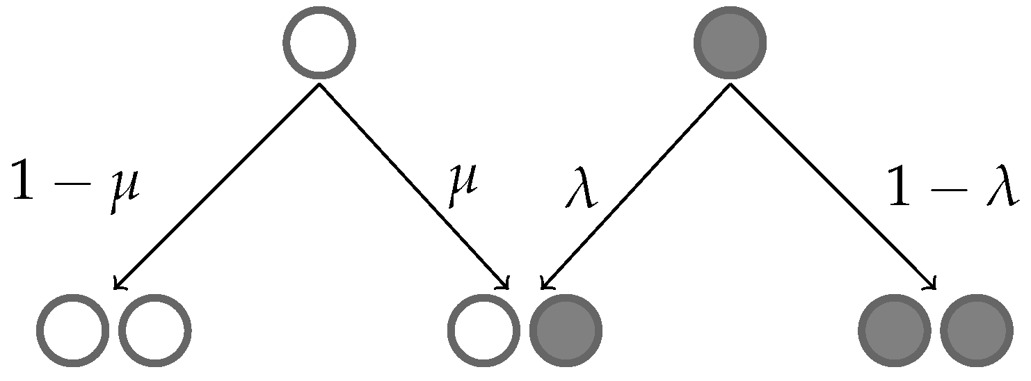
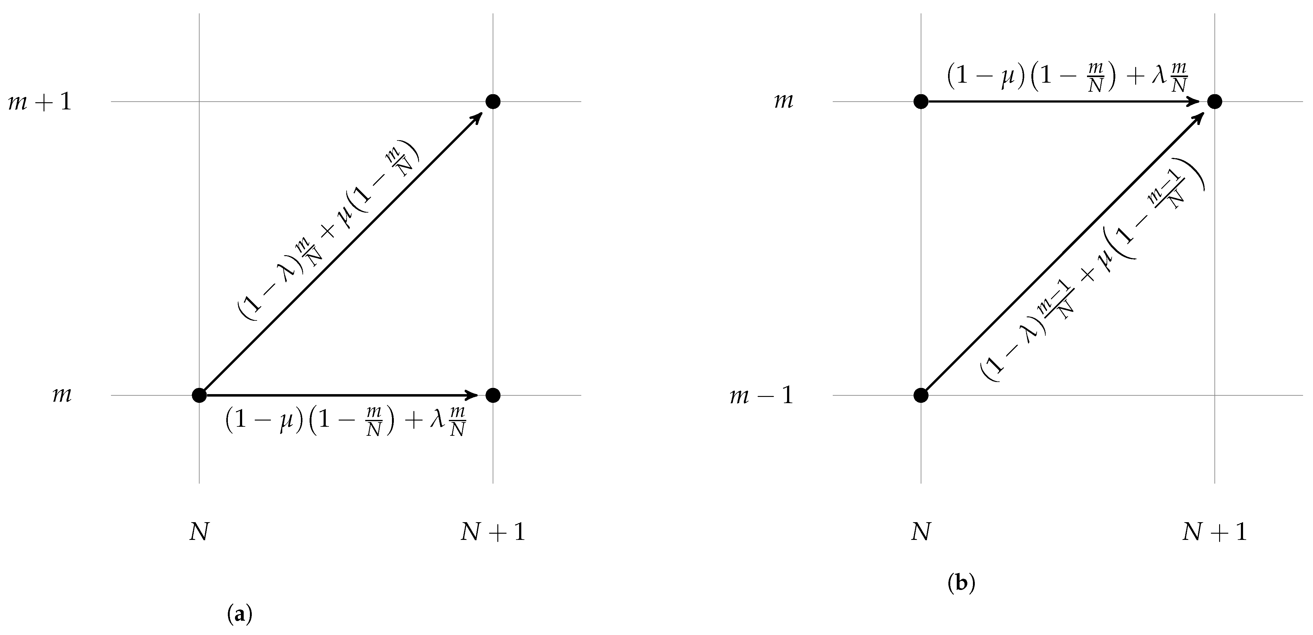
2. Model Formulation

The growing population of resistant and sensitive cells is modelled with a two-type branching process in continuous time [33]. In the model, each cell has an exponentially distributed cell-cycle duration that is independent of other cells in the population. We assumed that the mean cell cycle was the same for sensitive and resistant cells. Cells divide at the end of the cell cycle; the state of the daughter cell is chosen probabilistically depending on the mother cell, as given in Figure 1.
We consider this branching process at the time points of cell division. If there are N cells immediately before a cell division time point of which m are resistant, then the dividing cell is resistant with probability m / N and sensitive with complementary probability 1 m / N . As shown in Figure 1, the daughter cell is, thus, resistant with probability ( 1 λ ) m / N + μ ( 1 m / N ) or sensitive with complementary probability ( 1 μ ) ( 1 m / N ) + λ m / N . As the total population increases by 1 in the cell division event, the number of resistant cells can remain the same or increase by 1 depending on the state of the new cell (Figure 2a).
The aim of this paper was to characterise the probability P N ( m ) of observing m resistant cells as the total population reached N. This probability could be evaluated recursively with a variation in the above argument. In order to have m resistant cells in the population of N + 1 cells after a cell division event, we must have had m resistant cells before the division and added a sensitive cell or added an extra resistant cell to the m 1 resistant cells before the division (Figure 2b). Adding up the probabilities of these two options, P N ( m ) satisfies the master equation:
P N + 1 ( m ) = 1 N { P N ( m 1 ) [ μ ( N ( m 1 ) ) + ( 1 λ ) ( m 1 ) ] + P N ( m ) [ ( 1 μ ) ( N m ) + λ m ] } .
Equation (1) was considered in [34]. For λ = 0 , (1) is simplified into the master equation for the irreversible case as previously studied in [10].
Master Equation (1) is studied subject to the following boundary conditions:
P N ( m ) = 0 if m < 0 or m > N
and the following initial condition:
P N 0 ( m ) = 1 if m = m 0 , 0 otherwise ,
where N 0 , the initial population size; m 0 , the initial resistant subpopulation size.

3. Methods

Following the previous studies in [10,11] and empirical evidence [2], we assumed that the resistance acquisition and loss probabilities were small perturbation parameters μ 1 and λ 1 . The aim of this paper was to characterise the asymptotic behaviour of the solution to Master Equation (1) subject to (2) and (3) as the perturbation parameters tended to zero. Therefore, we assumed that they tended to zero with the same rate: μ / λ = O ( 1 ) .

3.1. Overview of Asymptotic Approximations

The problem in question is singularly perturbed, and there are several alternative distinguished approximations that apply to different regions of the definition domain 0 m N < of the solution P N ( m ) , and intermediate approximations through which the former can be matched. Additionally, the analysis proceeds differently depending on whether we start with a homogeneous population, i.e., with m 0 = 0 resistant and N 0 > 0 sensitive cells or m 0 = N 0 > 0 resistant cells, or we start with a mixed population with m 0 > 0 resistant and N 0 m 0 > 0 sensitive cells. Our aim was to treat all the possible combinations exhaustively; to help the reader in navigating through the resulting complexity, Table 1 outlines the region of validity for the individual approximations and gives references to their formulae. Below, we provide a brief commentary on the table. The derivations are found in the subsections that follow.
The first asymptotic approximation was developed under the assumption of bounded population sizes N = O ( 1 ) as the perturbation parameters tended to zero. The number of resistant cells was then also bounded via the natural constraint m N . Mathematically, the solution was developed into a regular power series in a perturbation parameter and approximated with the leading order term. Therefore, it is a regular approximation to the solution or simply regular solution. The approximation occupies the first row of Table 1 and is derived in Section 3.2.
Regular approximation is an example of a distinguished limit [35]: the variables are of definite order O ( 1 ) . Another distinguished limit occurs if the total population size N is inversely proportional to the small perturbation parameter while the number m of resistant cells is O ( 1 ) (Table 1, row 3, column 1). This is the large-population and low-mutation rate scenario discussed in previous works on the unidirectional case [10,11]. Given that m N , this scenario represents a left boundary layer of the definition interval 0 m N of the solution P N ( m ) . Our structurally symmetric model could also develop a right boundary layer in which the number N m of sensitive cells is O ( 1 ) (Table 1, row 3, column 3).
Three intermediate limits are obtained by taking the total large population in the regular solution and considering various scales of resistant and sensitive subpopulations (Table 1, row 2; Section 3.3, Section 3.4 and Section 3.5). The intermediate left and right regular solutions are used for the asymptotic matching of the distinguished left and right solutions (Section 3.6 and Section 3.7). The coarse-grained regular solution is applicable to the space between the two boundary layers (Table 1, row 3, middle column) and can be combined with the layer solutions into a uniform composite approximation (Section 3.8).
The triangular character of definition domain 0 m N < in Table 1 renders the concept of inner and outer solutions ambiguous. On the one hand, following [10], one can refer to the boundary layer solutions as inner because they focus on small fractions of the total population. On the other hand, following classical applications of singular perturbations in biology [36], one can also refer to the regular solution as inner because it captures the system’s early dynamics. In order to avoid a clash with earlier conventions, we do not use “inner and outer solutions” in this work.

3.2. Regular Solution

Through a regular solution to Master Equation (1), we find a solution that regularly depends on perturbation parameter μ , i.e., is a power series in μ . Our aim was to determine this solution at the leading order, i.e., to provide the first nonzero term of the power series. Cases m 0 > 0 and N 0 m 0 > 0 (initially present resistant and sensitive cells) were, perhaps surprisingly, easier than the m 0 = 0 and N 0 > 0 cases or the symmetrically opposite case of m 0 = N 0 > 0 , and were treated first.

3.2.1. Case m 0 > 0 and N 0 m 0 > 0

Rather than formally solving Difference Equation (1), it is both easier and more instructive to derive the regular solution from probabilistic considerations. The leading-order behaviour of the regular solution was obtained simply by neglecting perturbations μ and λ in (1). The resulting equation describes a growing culture of cells that deterministically pass their state to their progeny. Growth is as follows: one chooses a cell at random and looks at its state; the chosen cell is returned to the culture, and another cell (a daughter) is added that has the same state.
Aside from the terminology (cells = balls; state = colour), this is a classical Polya urn model [37]. A detailed description of this model can be found in Appendix A. As a result, with μ (and λ ) approaching zero,
P N ( m ) ( m 1 ) ! ( N m 1 ) ! ( N N 0 ) ! B ( m 0 , N 0 m 0 ) ( m m 0 ) ! ( N m N 0 + m 0 ) ! ( N 1 ) ! ,
where m 0 m N N 0 and the tilde sign are understood in the usual sense of asymptotic expansions [35]. B ( x , y ) = Γ ( x ) Γ ( y ) / Γ ( x + y ) = ( x 1 ) ! ( y 1 ) ! / ( x + y 1 ) ! is the beta function.

3.2.2. Case m 0 = 0 , N 0 > 0

The case of an entirely sensitive initial population is of prime interest here. It is more difficult than the mixed initial population case in Section 3.2.1. We used the previous case in deriving the new result. First, neglecting perturbations μ and λ in (1) leads to a problem with a trivial solution, namely, one always chooses a sensitive cell and keeps adding new sensitive cells. Mathematically,
P N ( 0 ) = 1 + O ( μ ) , P N ( m ) = O ( μ ) , m > 0 .
The second equation in (5) tells us that the probability of finding some sensitive cells is small, but does not describe the leading-order behaviour—here, O( μ ). For this, we needed a subtler estimate that we once again obtained from probabilistic considerations rather than formal solution techniques for difference equations.
Let L ˜ denote the population size, such that the first L ˜ cells are sensitive, and the ( L ˜ + 1 ) -th cell is resistant. Its distribution is shifted geometrically: Prob ( L ˜ = L ) = ( 1 μ ) L N 0 μ , L N 0 . Conditioning the value of L ˜ = L , we have
P N ( m ) = L = N 0 N m P ( m , N | 1 , L + 1 ) ( 1 μ ) L N 0 μ ,
where P ( m , N | 1 , L + 1 ) denotes the probability of observing m resistant cells in a population of size N that was initially of size L + 1 and contained one resistant cell. This can be estimated by setting m 0 = 1   N 0 = L + 1 into (4), which yields
P ( m , N | 1 , L + 1 ) L ( N m 1 ) ! ( N L 1 ) ! ( N 1 ) ! ( N m L ) ! .
Since the main aim was to derive a leading-order approximation of P N ( m ) , we could neglect μ in the factors ( 1 μ ) appearing in (6). As a result, we obtained
P N ( m ) μ ( N m 1 ) ! ( N 1 ) ! L = N 0 N m L ( N L 1 ) ! ( N m L ) ! .
Moreover, using symbolic software (details in Appendix B), the sum appearing in the previous equation can be simplified as follows:
L = N 0 N m L ( N L 1 ) ! ( N L m ) ! = ( N N 0 ) ! ( N m + m N 0 ) m ( m + 1 ) ( N N 0 m ) ! ,
giving the final result
P N ( m ) μ ( N N 0 ) ! ( N m 1 ) ! ( N m + m N 0 ) m ( m + 1 ) ( N 1 ) ! ( N N 0 m ) ! , m > 0 .
Formula (10) was derived with other means for the unidirectional model in [10].

3.2.3. Case m 0 = N 0 > 0

This case is a mirror reflection of the case discussed in Section 3.2.2. The result, which reads P N ( N ) 1 and
P N ( m ) λ ( N N 0 ) ! ( m 1 ) ! ( m + ( N m ) N 0 ) ( N m ) ( N m + 1 ) ( N 1 ) ! ( m N 0 ) ! , m < N ,
was readily obtained by replacing μ by λ , N 0 m 0 by m 0 , N m by m, and vice versa in (10).

3.3. Regular Left Solution

A regular left solution means the approximate solution that considers a relatively large total population 1 N 1 μ that includes only a small number of resistant cells m = O ( 1 ) . The regular left solution can be derived from regular solution Formulae (4), (10), and (11) by approximating descending factorials by powers as appropriate; for example, one has
( N N 0 ) ! ( N 1 ) ! = 1 ( N 1 ) ( N 2 ) ( N N 0 + 1 ) 1 N N 0 1
for N 1 .
  • Case m 0 > 0 and N 0 m 0 > 0
    P N ( m ) ( m 1 ) ( m 2 ) ( m m 0 + 1 ) N m 0 B ( m 0 , N 0 m 0 ) .
  • Case m 0 = 0 , N 0 > 0
    P N ( m ) 1 if m = 0 , μ N m ( m + 1 ) otherwise .
  • Case m 0 = N 0 > 0
    P N ( m ) λ N 0 ( m 1 ) ( m 2 ) ( m N 0 + 1 ) N N 0 .

3.4. Regular Right Solution

A regular right solution is the approximate solution that considers a relatively large total population, 1 N 1 μ that includes a large number of resistant cells; mathematically, N m = O ( 1 ) . These approximations are most conveniently obtained by performing substitutions m N m , m 0 N 0 m 0 , and λ μ in (13), (14), and (15).

3.4.1. Case m 0 > 0 and N 0 m 0 > 0

The approximation reads
P N ( m ) ( N m 1 ) ( N m 2 ) ( N m ( N 0 m 0 ) + 1 ) N N 0 m 0 B ( m 0 , N 0 m 0 ) .

3.4.2. Case m 0 = 0 , N 0 > 0

The approximation reads
P N ( m ) μ N 0 ( N m 1 ) ( N m 2 ) ( N m N 0 + 1 ) N N 0 .

3.4.3. Case m 0 = N 0 > 0

The approximation reads
P N ( m ) λ N ( N m ) ( N m + 1 ) if m < N , 1 if m = N .

3.5. Regular Coarse-Grained Solution

A regular coarse-grained solution is an approximate solution that considers a large number of cells in the total population, while the order of the number of resistant and sensitive cells in the population is the same. Mathematically, m = O ( N ) = N m . The regular coarse-grained solution was obtained, similarly as regular left/right solutions, by approximating descending factorials by appropriate powers in regular solution Formulas (4), (10), and (11). For example,
( N m 1 ) ! ( N m N 0 + m 0 ) ! = ( N m 1 ) ( N m 2 ) ( N m N 0 + m 0 + 1 ) ( N m ) N 0 m 0 1
holds for m and N both large and of the same order.

3.5.1. Case m 0 > 0 and N 0 m 0 > 0

The approximation reads
P N ( m ) m m 0 1 ( N m ) N 0 m 0 1 N N 0 1 B ( m 0 , N 0 m 0 ) .

3.5.2. Case m 0 = 0 , N 0 > 0

The approximation reads
P N ( m ) μ ( N m + m N 0 ) m 2 1 m N N 0 1 .

3.5.3. Case m 0 = N 0 > 0

The approximation reads
P N ( m ) λ ( m + ( N m ) N 0 ) ( N m ) 2 m N N 0 1 .
The (20) relates to the classical convergence result to the beta distribution for the Polya urn [38]; (21) and (22) are symmetric.

3.6. Left Boundary Layer Solution

As in the previous sections, we assumed that the resistance acquisition and loss probabilities were small, i.e., μ 1 and λ 1 such that λ / μ = O ( 1 ) , and that the total population size was large, i.e., N 1 . In contrast with the previous sections, here, we focus on the distinguished large-population low-mutation-rate regime in which the population is so large as to produce the population rates of resistance acquisition and loss
y = μ N , y ˜ = λ N ,
of order 1. The distinguished limit was found for m = O ( 1 ) resistant cells. This represents a (left) boundary layer of the large interval of admissible values m { 0 , 1 , , N } . The right boundary layer occurring for N m = O ( 1 ) is treated in the next section with symmetry arguments. Unless stated otherwise, asymptotic equivalence sign ∼ is used in this section in the context of limit process μ 0 , y = O ( 1 ) , y ˜ = O ( 1 ) , m = O ( 1 ) .
The boundary-layer solution is found with the method of the generating function, which is defined via
G N ( x ) = m = 0 N P N ( m ) x m .
The usual rules [39] transform Master Equation (1) into a difference–differential equation:
N ( G N + 1 ( x ) G N ( x ) ) = ( x 1 ) ( μ N + ( 1 μ λ ) x x ) G N ( x )
for the generating function.
Guided by Intermediate Asymptotics (13), (14), and (15) of the regular solution, we looked for a generating function with the same kind of asymptotics:
G N ( x ) N β H ( x , y ) , 0 < x < 1 ,
where β is to be matched to a regular solution.
G N + 1 ( x ) = ( N + 1 ) β H ( x , y ( 1 + 1 / N ) ) N β H + N β 1 ( β H + y y H ) + O ( N β 2 ) .
Inserting (26) and (27) into (25), and collecting leading order terms, we obtained the following partial differential equation:
β H + y y H = ( x 1 ) ( y + x x ) H .
For β = 0 , (28) is the Lea–Coulson equation [9]. Parameter β can be viewed as an eigenvalue, and solution H as an eigenfunction of the Lea–Coulson differential operator.
Solving (28) with the method of characteristics, one uncovers the following parametric family of solutions:
H ( x , y ) = C y γ x 1 x β γ ( 1 x ) y ( 1 x ) / x ,
where C and γ are arbitrary constants. In what follows, we determine these constants and eigenvalue β by matching them to the regular solution. The distinct previously introduced cases were thereby treated separately.

3.6.1. Case m 0 > 0 , N 0 m 0 > 0

The limiting operations of infinite summation (to obtain a generating function from a sequence of probabilities) and the asymptotic limit process can be interchanged for x < 1 using a dominated convergence-type argument. Specifically, the left–regular approximation (13) can be expressed in terms of the generating function as follows:
G N ( x ) N m 0 Γ ( N 0 ) Γ ( N 0 m 0 ) x 1 x m 0 , 0 < x < 1 .
The approximation is valid in the left boundary layer m = O ( 1 ) for an intermediate range of population sizes 1 N 1 / μ .
Matching (30) with (26) and (29) yields γ = 0 , β = m 0 , and C = Γ ( N 0 ) / Γ ( N 0 m 0 ) , i.e.,
G N ( x ) N m 0 Γ ( N 0 ) Γ ( N 0 m 0 ) x 1 x m 0 ( 1 x ) y ( 1 x ) / x , 0 < x < 1 ,
which is valid in the left boundary layer m = O ( 1 ) for population sizes extending up to N = O ( 1 / μ ) .
The right-hand side of (31) can be transformed into the probability space by combining the following rules:
  • x transforms into the shift operator.
  • ( 1 x ) 1 transforms into the summation operator (a discrete convolution with a sequence of ones).
  • ( 1 x ) k transforms into the kth power of this operator (a discrete convolution with the sequence { Γ ( k + m ) / Γ ( k ) m ! } m 0 ).
  • ( 1 x ) y ( 1 x ) / x transforms into the Lea–Coulson probability mass function (PMF).
Therefore, Approximation (31), when expressed in terms of the probability mass function, reads
P N ( m ) N m 0 Γ ( N 0 ) Γ ( N 0 m 0 ) P L C ( m 0 ) ( m m 0 ; y ) ,
where P L C ( k ) ( m ; y ) is the kth summation of the Lea–Coulson probability mass function, i.e.,
P L C ( 0 ) ( m ; y ) = x m ( 1 x ) y ( 1 x ) / x m ! x = 0 ,
P L C ( k ) ( m ; y ) = j = 0 m P L C ( k 1 ) ( j ; y ) = j = 0 m Γ ( k + m ) Γ ( k ) m ! P L C ( 0 ) ( m j ; y ) , k = 1 , 2 ,
In particular, P L C ( 0 ) ( m ; y ) is the Lea–Coulson PMF and P L C ( 1 ) ( m ; y ) is the Lea–Coulson cumulative distribution function (CDF).

3.6.2. Case m 0 = 0 , N 0 > 0

The left-regular intermediate approximation (14) implies G N ( x ) 1 for 1 N 1 / μ at leading order. Matching this to (29) and (26) gives β = γ = 0 , C = 1 . The left boundary approximation then reads
G N ( x ) ( 1 x ) y ( 1 x ) / x
in the generating function space and
P N ( m ) P L C ( 0 ) ( m ; y )
in the probability space. In this case, the matching procedure is equivalent to directly imposing the initial condition (of starting without any resistant cells) on the solution to the Lea–Coulson equation [10].

3.6.3. Case m 0 = N 0 > 0

Intermediate Approximation (15) implies
G N ( x ) y ˜ N N 0 1 Γ ( N 0 + 1 ) x 1 x N 0 , 0 < x < 1 ,
for 1 N 1 / μ . Matching with (29) and (26) yields γ = 1 , β = N 0 + 1 , C = Γ ( N 0 + 1 ) λ / μ , i.e.,
G N ( x ) y ˜ N N 0 1 Γ ( N 0 + 1 ) x 1 x N 0 ( 1 x ) y ( 1 x ) / x , 0 < x < 1 .
This reads
P N ( m ) y ˜ N N 0 1 Γ ( N 0 + 1 ) P L C ( N 0 ) ( m N 0 ; y )
in the probability space.

3.7. Right Boundary Layer Solution

Symmetry considerations imply that P N ( m ) = P ¯ N ( N m ) , where the bar indicates a model in which the substitutions m 0 N 0 m 0 and λ μ ( y ˜ y ) are performed. Combining the symmetry result with the previous section’s results on the left boundary layer yields the following list of approximations. The equivalence sign is used in the context of μ 0 , y = O ( 1 ) , y ˜ = O ( 1 ) , N m = O ( 1 ) .

3.7.1. Case m 0 > 0 , N 0 m 0 > 0

The approximation reads
P N ( m ) N N 0 + m 0 Γ ( N 0 ) Γ ( m 0 ) P L C ( N 0 m 0 ) ( N m N 0 + m 0 ; y ˜ ) .

3.7.2. Case m 0 = 0 , N 0 > 0

The approximation reads
P N ( m ) y N N 0 1 Γ ( N 0 + 1 ) P L C ( N 0 ) ( N m N 0 ; y ˜ ) .

3.7.3. Case m 0 = N 0 > 0

The approximation reads
P N ( m ) P L C ( 0 ) ( N m ; y ˜ ) .

3.8. Log-Composite Solution

Composite solutions provide a means of combining multiscale asymptotic approximations into a single uniformly valid approximation. Typically, the composite solution is equal to the sum of the inner and outer solutions minus their common limit value in the overlap region; this construction was applied to, e.g., enzyme kinetics [36] and the mathematical analysis of a hematopoietic genetic switch [40]. In a log-composite solution, addition and subtraction are replaced by multiplication and division.
For N = O ( 1 / μ ) , three approximations are available in different sections of the definition domain m { 0 , 1 , , N } : the left boundary layer solution applies to m = O ( 1 ) ; the regular coarse-grained solution applies to m = O ( N ) = N m ; the right boundary layer solution applies to N m = O ( 1 ) . Table 1, row 3, contains references to the specific formulae for the mixed and exclusively sensitive initial conditions. The product of these three approximations provides the numerator of the log-composite solution, which is constructed according to the following scheme:
P N ( m ) left × regular coarse - grained × Right left overlap × right overlap ,
in which the ‘left’, ’right’, and ’regular coarse-grained’ labels are replaced with the appropriate formulae in the usual cases of different initial conditions. Let us now define the ‘left overlap’ and ’right overlap’ terms in the denominator; for concreteness, consider the case m 0 = 0 of a sensitive initial population. The overlap between Left Solution (36) and Regular Coarse-Grained Solution (21) can be obtained by taking m in the former or m 0 in the latter; both procedures yield the same left overlap solution P N ( m ) μ N / m 2 [23] because of the asymptotic matching principle [35]. Similarly, taking N m in Right Solution (41) or N m 0 in the Regular Coarse-Grained Solution (21) yields right overlap solution P N ( m ) μ N 0 ( 1 m / N ) N 0 1 / N . For any value of m, one of the three factors in the numerator of (43) provides a valid approximation to the exact distribution, while the two remaining factors reduce to their overlap form and cancel with the denominator. Thus, Formula (43) provides a uniform approximation across the entire interval of admissible values of m.
The application of Pattern (43) in the usual cases leads to the following.

3.8.1. Case m 0 > 0 , N 0 m 0 > 0

The approximation reads
P N ( m ) N N 0 + 1 Γ ( N 0 ) P L C ( m 0 ) ( m m 0 ; y ) P L C ( N 0 m 0 ) ( N m N 0 + m 0 ; y ˜ ) .

3.8.2. Case m 0 = 0 , N 0 > 0

The approximation reads
P N ( m ) N N 0 + 1 Γ ( N 0 ) P L C ( 0 ) ( m ; y ) 1 + ( N 0 1 ) m N P L C ( N 0 ) ( N m N 0 ; y ˜ ) .

3.8.3. Case m 0 = N 0 > 0

The approximation reads
P N ( m ) N N 0 + 1 Γ ( N 0 ) P L C ( N 0 ) ( m N 0 ; y ) N 0 ( N 0 1 ) m N P L C ( 0 ) ( N m ; y ˜ ) .

3.9. Landau Distribution

As the shape parameter y of the Lea–Coulson PMF P L C ( 0 ) ( m ; y ) increases, the PMF can be approximated with the probability density function (PDF) of the Landau distribution [10]. Additionally, partial summation P L C ( k ) ( m ; y ) , k = 1 , 2 , can be approximated with the partial integration of the PDF. Precisely,
P L C ( k ) ( m k ; y ) y k 1 F Landau ( k ) m y ln y ,
where
F Landau ( 0 ) ( ξ ) = f Landau ( ξ ) = 1 π 0 exp ( v ( ξ + ln v ) ) sin ( π v ) d v
is the density of Landau distribution [26,41] and
F Landau ( k ) ( ξ ) = ξ F Landau ( k 1 ) ( ξ ˜ ) d ξ ˜ = 1 Γ ( k ) ξ ξ ˜ k 1 f Landau ( ξ ξ ˜ ) d ξ ˜
is the kth partial integration of the density. In particular, F Landau ( ξ ) = F Landau ( 1 ) ( ξ ) is the CDF of the Landau distribution.

4. Results

This paper provides asymptotic approximations to the Luria–Delbrück distribution P N ( m ) of observing m resistant cells as the total population reaches size N. Specifically, distribution P N ( m ) is defined as the solution to Master Equation (1), subject to boundary and initial Conditions (2)–(3). The input parameters of the distribution were the final population size N and the probabilities μ and λ of resistance acquisition and loss, respectively. In the examples below, we adopt the values N = 2 × 10 5 and μ = 10 3 from the study of the unidirectional model [10]; we compare the unidirectional ( λ = 0 ) and bidirectional ( λ = 10 3 ) cases.
The distribution P N ( m ) also depends on the initial population size N 0 and the initial number of resistant cells m 0 . In the following subsections, we report the distribution asymptotics for initial conditions of increasing complexity. Section 4.1 deals with a population that starts from a single sensitive cell ( N 0 = 1 , m 0 = 0 ). Section 4.2 focuses on a population that begins with two cells of different kinds ( N 0 = 2 , m 0 = 1 ). The case of a general (deterministic) initial condition is outlined in Section 4.3. Section 4.4 briefly considers the case of a nondeterministic initial condition.

4.1. One Sensitive Cell at the Beginning

This type of initial condition has been widely considered in studies concerning the Luria–Delbrück fluctuation test. Approximations of the resistant population distribution by the Lea–Coulson probability mass function and the Landau probability density function were reported. This paper establishes the appearance of partial summations/integrations of these distributions, in particular the cumulative distribution function, in the tail of the population distribution.
For low-to-moderate values m, the probability of seeing m resistant cells among N total cells is approximated with the following (see Figure 3a):
P N ( m ) 1 μ N f Landau m μ N ln μ N ,
where f Landau ( ξ ) is Density (48) of Landau distribution. The approximation follows from (36) and (47). This approximation was previously derived for the unidirectional model in [10].
For a large number of resistant cells m in the population, we have the following approximation (see Figure 3b):
P N ( m ) μ N F Landau N m λ N ln λ N ,
where F Landau ( x ) = x f Landau ( y ) d y is the cumulative distribution function of Landau distribution. The approximation follows from (41) for N 0 = 1 and (47).
Lastly, the following composite approximation (Figure 3c):
P N ( m ) 1 μ N f Landau m μ N ln μ N F Landau N m λ N ln λ N
works well for all possible numbers m of resistant cells. The approximation follows from (45) for N 0 = 1 and (47).
In the irreversible and unidirectional case ( λ = 0 ), Landau PDF (50) applies uniformly for the entire range of 0 m < N of resistant subpopulation sizes (Figure 3d–f). The probability distribution then exhibits a sharp cut-off at m = N (Figure 3e); contrastingly, the presence of a reverse transition smooths the cut-off into a Landau CDF in the right boundary layer (Figure 3b).

4.2. One Sensitive and One Resistant Cell at the Beginning

A mixed model develops a dramatically different dynamics than the homogeneous initial population. In an initial phase, which lasts until the population size reaches the reciprocal of the small resistance acquisition parameter, the dynamics are driven by the competition between the independent progeny of the two parent cells. A classical result implies that this tug of war leads to the uniform distribution of resistant/sensitive cells [38]. In this paper, this classical result was incorporated into Regular Coarse-Grained Approximation (20) with m 0 = 1 , N 0 = 2 . After the initial phase, boundary layers appeared at the left and right corners of m { 0 , 1 , , N } due to resistance acquisition and loss. This paper provides nontrivial approximations of the boundary behaviour through the Landau cumulative distribution function.
For a small-to-moderate number of resistant cells m in the population, we have the following approximation (Figure 4a):
P N ( m ) 1 N F Landau m μ N ln μ N .
The approximation was derived from (32) for m 0 = 1 , N 0 = 2 and (47).
For a large number of resistant cells m in the population, we have the following approximation (Figure 4b):
P N ( m ) 1 N F Landau N m λ N ln λ N .
The approximation was derived from (40) for m 0 = 1 , N 0 = 2 and (47).
Lastly, just like in the case of a sensitive initial population, in the case of a mixed initial population, one can find a composite approximation that works very well for all possible m. In this case, it is given by (Figure 4c):
P N ( m ) 1 N F Landau m μ N ln μ N F Landau N m λ N ln λ N .
The approximation was derived from (44) for m 0 = 1 , N 0 = 2 and (47).
In the unidirectional case ( λ = 0 ), the Landau CDF approximation (50) applied uniformly to all resistant subpopulation sizes 0 m < N (Figure 4d–f). Again, a sharp cut-off was observed at m = N in the unidirectional case (Figure 4e), whereas a Landau CDF in the right boundary layer appeared in the reversible case (Figure 4b).

4.3. More than One Sensitive or Resistant Cells at the Beginning

The cumulative distribution function is a partial integration (up to a given level) of the probability density function. The second, third, etc. partial integrations are defined recursively. The higher-order integrations of Landau density appear in the boundary behaviour of the Luria–Delbrück distribution if the initial condition contains more than one cell of either type (resistant/sensitive).
For the sake of brevity, we only give the composite approximations. If we initially have m 0 = 0 resistant and N 0 > 0 sensitive cells, then (52) generalises to
P N ( m ) Γ ( N 0 ) λ N 0 1 μ N f Landau m μ N ln μ N 1 + ( N 0 1 ) m N F Landau ( N 0 ) N m λ N ln λ N ,
If we initially have m 0 > 0 resistant and N 0 m 0 > 0 sensitive cells, on the other hand, then (55) generalises to
P N ( m ) Γ ( N 0 ) μ m 0 1 λ N 0 m 0 1 N F Landau ( m 0 ) m μ N ln μ N F Landau ( N 0 m 0 ) N m λ N ln λ N .
Equations (56)–(57) were derived by combining (44)–(45) with (47); Γ stands for the gamma function, and F Landau ( k ) gives the k-th partial integration (49) of the Landau probability density function.

4.4. Stochastic Initial Conditions

Our analysis so far concerned deterministic initial Condition (3). A previous study of a bidirectional model (based on different assumptions) [8] considered a stochastic initial condition in which the population was derived from a single initial cell, which could be with a certain probability ρ sensitive; with the complementary probability, it is resistant. Via the superposition principle, the solution that is subject to the stochastic initial condition is equal to the weighted sum of the solution starting deterministically with one sensitive parent and the solution starting deterministically with one resistant parent. The Landau cumulative distribution functions in the tails of the two solutions are then negligible. For low-to-moderate values m, the probability of seeing m resistant cells among N total cells is approximated as follows:
P N ( m ) ρ μ N f Landau m μ N ln μ N .
For a large number of resistant cells m in the population, we have the following approximation:
P N ( m ) 1 ρ λ N f Landau N m λ N ln λ N .
A uniformly valid solution is obtained by adding up (58) and (59):
P N ( m ) ρ μ N f Landau m μ N ln μ N + 1 ρ λ N f Landau N m λ N ln λ N .
This is a composite rather than log-composite approximation.
A special type of initial condition is if the switching between resistance and sensitivity is in balance: ρ = λ / ( μ + λ ) , 1 ρ = μ / ( μ + λ ) . Then, the mean resistant fraction satisfies m = 0 N m P N ( m ) / N = μ / ( μ + λ ) , i.e., it does not change as the population grows [8].

4.5. Limitations of the Approximations

The left boundary solution has the form of the Landau PDF/CDF located at m = μ N ln μ N ; see Equations (50), (53) and (58). For self-consistency, we required that the boundary layer location be much lower than the size of the entire definition domain, meaning that μ N ln μ N N . This is equivalent to requiring ln N 1 / μ , where μ 1 . Thus, N should be large but not exponentially large for the asymptotic approximations to apply.

5. Discussion

The paper focused on a stochastic Luria–Delbrück fluctuation test model with reversible switching between two cellular states (for example, single cells being drug-resistant or drug-sensitive). We considered a fixed-population ensemble formulation in which the population was expanded until it had reached a given size. The main contribution of the paper is the characterisation of the Luria–Delbrück distribution of resistant cells in the final population. We focused on the parametric regime of low switching probabilities and large populations; we used singular perturbation methods to obtain asymptotic approximations to the desired distribution. The novelty of the work lies in the systematic use of asymptotic matching between the alternate approximations. The approach is applicable to other known approximations, e.g., Fréchet distribution [42].
While our analysis focused on a fixed-population ensemble, the results also have implications in the case of a fixed-time ensemble. In the latter formulation, the population is grown until a fixed end time point, as explained in Section 2. The total population grows exponentially as per the Yule growth process with a reciprocal growth rate to the mean generation time. If one conditions on the Yule process reaching a given value N, one recovers the fixed-ensemble model for the number of resistant cells as studied in this paper.Conversely, drawing N from the state of a Yule growth process at a given time t, the fixed-population ensemble is turned into a fixed-time ensemble formulation. Conditioning a fixed population thus eliminates proliferation noise. Another approach to this consists of calculating the relative fractions of sensitive/resistant cells [8].
Our model assumes that switching between sensitivity and resistance occurs at cell division events. A previous study [8] of a reversible switching case was based on different assumptions that warrant a brief discussion. Like in the fixed time ensemble version of our model, the cell cycle was assumed to be exponentially distributed, and the mean generation time was the same for the two cell types. However, switching was uncoupled from the cell cycle in [8]: a daughter cell is always of the same type as the mother cell, and any cell has a constant propensity to transition at any time to the opposite state.
Importantly, unlike in our model, there could be more than one switching event per cell cycle in the model of [8]. Therefore, although this needs to be supported by further analysis, the difference between the two formulations is expected to be pronounced in the fast switching regime in which multiple switching events per cell cycle are probable. In the model of [8], proliferation events increased the population by one, but the switching events did not; this renders the relationship between the fixed-time and fixed-population ensemble formulations subtler. Further complications in the dynamics arise if the switching rates depend on the presence of drugs [43,44].
The reversible model studied in this paper is a direct extension of the irreversible switching model studied in [10]; indeed, setting probability λ that a resistant mother bears a sensitive daughter cell to zero, one recovers the earlier model. The earlier study provides methods that are specifically applicable to the important regime of a large population subject to low-rate switching. We extended these methods to the current reversible case. The generalisation required nontrivial modifications in the methodology, notably in the systematic use of asymptotic matching between the small and large population solutions.
The new approximation differs from that given in [10] only regarding the low-probability distribution tail, as evidenced in Figure 3. Nevertheless, the appearance of the Landau cumulative distribution function in the tail is widely interesting. Additionally, we established that it also appeared for mixed initial conditions, as illustrated in Figure 4.

6. Conclusions

In this paper, we theoretically showed that reversible switching in a fluctuation test experiment affects the tail of Luria–Delbrück distribution. Methodologically, our results were based on the matched asymptotic framework that allows for alternate approximations to the distribution under different parameter scaling regimes, combining them into a uniform composite approximation. We expect that the approach could be extended, particularly to more complicated (and realistic) descriptions of the fluctuation test experiment, and provide valuable insights into the underlying dynamics.

Author Contributions

Conceptualization, A.S.; methodology, P.B.; analysis, P.B. and A.H.; visualization, A.H.; writing—review and editing, P.B., A.H. and A.S. All authors have read and agreed to the published version of the manuscript.

Funding

This research was supported by the Slovak Research and Development Agency under contract no. APVV-18-0308, and VEGA grants 1/0339/21 and 1/0755/22. A.S. acknowledges support from ARO W911NF-19-1-0243, and NIH grants R01GM124446 and R01GM126557.

Institutional Review Board Statement

Not applicable.

Data Availability Statement

Not applicable.

Acknowledgments

The authors are grateful to the three anonymous referees whose insightful review reports helped in improving the manuscript.

Conflicts of Interest

The authors declare no conflict of interest. The funders had no role in the design of the study; in the collection, analyses, or interpretation of data; in the writing of the manuscript; or in the decision to publish the results.

Abbreviations

The following abbreviations are used in this manuscript:
PMFProbability mass function
PDFProbability density function
CDFCumulative distribution function
L–CLea–Coulson

Appendix A. Polya urn Models

Suppose that we have an urn that first consists of w white balls and b black balls. Then, we withdraw a ball from the urn one at a time, look at its colour, return the ball to the urn, and add c balls of the same colour. The probability that x white balls are drawn in a sample of n withdrawals is
P [ X = x ] = w c + x 1 x b c + n x 1 n x w + b c + n 1 n .
The number of balls of a specific colour in the Polya urn model follows negative hypergeometric distribution [37].
We can adapt the Polya urn model to our situation in the following way. First, c = 1 in our case, as in every birth event, and only one new cell is born. Furthermore, w and b are the number of resistant and sensitive cells in the initial population, respectively; n denotes the number of birth events, and x denotes the number of resistant cells among these n births. The following relations with the notation used in the main text hold:
m 0 = w , N 0 = b + w , m = w + x , N = w + b + n .
Therefore, we can write that, as μ (and λ ) tends to zero,
P N ( m ) m 1 m m 0 N m 1 N m ( N 0 m 0 ) N 1 N N 0 , where m 0 m N N 0 ,
where the tilde sign is understood in the usual sense of asymptotic expansions. The rearrangement of combinatorial numbers yields (4).

Appendix B. Computations

The symbolic computation of Sum (9) was performed using MATLAB’s Symbolic Math Toolbox [45]:
Axioms 12 00249 i001

References

  1. Luria, S.E.; Delbrück, M. Mutations of bacteria from virus sensitivity to virus resistance. Genetics 1943, 28, 491. [Google Scholar] [CrossRef] [PubMed]
  2. Shaffer, S.M.; Dunagin, M.C.; Torborg, S.R.; Torre, E.A.; Emert, B.; Krepler, C.; Beqiri, M.; Sproesser, K.; Brafford, P.A.; Xiao, M.; et al. Rare cell variability and drug-induced reprogramming as a mode of cancer drug resistance. Nature 2017, 546, 431–435. [Google Scholar] [CrossRef] [PubMed] [Green Version]
  3. Shaffer, S.M.; Emert, B.L.; Hueros, R.A.R.; Cote, C.; Harmange, G.; Schaff, D.L.; Sizemore, A.E.; Gupte, R.; Torre, E.; Singh, A.; et al. Memory sequencing reveals heritable single-cell gene expression programs associated with distinct cellular behaviors. Cell 2020, 182, 947–959. [Google Scholar] [CrossRef] [PubMed]
  4. Hossain, T.; Singh, A.; Butzin, N.C. Escherichia coli cells are primed for survival before lethal antibiotic stress. bioRxiv 2022. [Google Scholar] [CrossRef]
  5. Chang, C.A.; Jen, J.; Jiang, S.; Sayad, A.; Mer, A.S.; Brown, K.R.; Nixon, A.M.; Dhabaria, A.; Tang, K.H.; Venet, D.; et al. Ontogeny and vulnerabilities of drug-tolerant persisters in her2+ breast cancer. Cancer Discov. 2022, 12, 1022–1045. [Google Scholar] [CrossRef]
  6. Harmange, G.; Hueros, R.A.R.; Schaff, D.L.; Emert, B.L.; Saint-Antoine, M.M.; Nellore, S.; Fane, M.E.; Alicea, G.M.; Weeraratna, A.T.; Singh, A.; et al. Disrupting cellular memory to overcome drug resistance. bioRxiv 2022. [Google Scholar] [CrossRef]
  7. Saint-Antoine, M.M.; Grima, R.; Singh, A. A fluctuation-based approach to infer kinetics and topology of cell-state switching. bioRxiv 2022. [Google Scholar] [CrossRef]
  8. Saint-Antoine, M.M.; Singh, A. Moment-based estimation of state-switching rates in cell populations. bioRxiv 2022. [Google Scholar] [CrossRef]
  9. Zheng, Q. Progress of a half century in the study of the Luria–Delbrück distribution. Math. Biosci. 1999, 162, 1–32. [Google Scholar] [CrossRef] [Green Version]
  10. Kessler, D.A.; Levine, H. Large population solution of the stochastic Luria–Delbrück evolution model. Proc. Natl. Acad. Sci. USA 2013, 110, 11682–11687. [Google Scholar] [CrossRef] [Green Version]
  11. Keller, P.; Antal, T. Mutant number distribution in an exponentially growing population. J. Stat. Mech. Theory Exp. 2015, 2015, P01011. [Google Scholar] [CrossRef] [Green Version]
  12. Nicholson, M.D.; Antal, T. Universal asymptotic clone size distribution for general population growth. Bull. Math. Biol. 2016, 78, 2243–2276. [Google Scholar] [CrossRef] [Green Version]
  13. Pakes, A.G. Mutant number laws and infinite divisibility. Axioms 2022, 11, 584. [Google Scholar] [CrossRef]
  14. Antal, T.; Krapivsky, P. Exact solution of a two-type branching process: Models of tumor progression. J. Stat. Mech. Theory Exp. 2011, 2011, P08018. [Google Scholar] [CrossRef]
  15. Angerer, W.P. An explicit representation of the Luria–Delbrück distribution. J. Math. Biol. 2001, 42, 145–174. [Google Scholar] [CrossRef] [PubMed]
  16. Kessler, D.A.; Levine, H. Scaling solution in the large population limit of the general asymmetric stochastic Luria–Delbrück evolution process. J. Stat. Phys. 2015, 158, 783–805. [Google Scholar] [CrossRef] [PubMed] [Green Version]
  17. Armitage, P. The statistical theory of bacterial populations subject to mutation. J. R. Stat. Soc. Ser. B (Methodol.) 1952, 14, 1–33. [Google Scholar] [CrossRef]
  18. Jolly, C.; Cook, A.; Raferty, J.; Jones, M. Measuring bidirectional mutation. J. Theor. Biol. 2007, 246, 269–277. [Google Scholar] [CrossRef]
  19. Sorace, R.; Komarova, N.L. Accumulation of neutral mutations in growing cell colonies with competition. J. Theor. Biol. 2012, 314, 84–94. [Google Scholar] [CrossRef] [Green Version]
  20. Cheek, D.; Antal, T. Genetic composition of an exponentially growing cell population. Stoch. Process. Their Appl. 2020, 130, 6580–6624. [Google Scholar] [CrossRef]
  21. Lea, D.E.; Coulson, C.A. The distribution of the numbers of mutants in bacterial populations. J. Genet. 1949, 49, 264–285. [Google Scholar] [CrossRef] [PubMed]
  22. Zheng, Q. A fresh approach to a special type of the Luria–Delbrück distribution. Axioms 2022, 11, 730. [Google Scholar] [CrossRef]
  23. Pakes, A.G. Remarks on the Luria–Delbrück distribution. J. Appl. Probab. 1993, 30, 991–994. [Google Scholar] [CrossRef] [Green Version]
  24. Angerer, W.P. A note on the evaluation of fluctuation experiments. Mutat. Res. Mol. Mech. Mutagen. 2001, 479, 207–224. [Google Scholar] [CrossRef] [PubMed]
  25. Bulyak, E.; Shul’ga, N. Landau distribution of ionization losses: History, importance, extensions. arXiv 2022, arXiv:2209.06387. [Google Scholar]
  26. Nolan, J.P. Univariate Stable Distributions; Springer: Berlin/Heidelberg, Germany, 2020. [Google Scholar]
  27. Rao, C.R.; Shanbhag, D.N.; Sapatinas, T.; Rao, M.B. Some properties of extreme stable laws and related infinitely divisible random variables. J. Stat. Plan. Inference 2009, 139, 802–813. [Google Scholar]
  28. Bender, C.M.; Orszag, S.A. Advanced Mathematical Methods for Scientists and Engineers I: Asymptotic Methods and Perturbation Theory, 1st ed.; Springer Science & Business Media: Berlin/Heidelberg, Germany, 1999. [Google Scholar]
  29. Hinch, E.J. Perturbation Methods; Cambridge University Press: Cambridge, UK, 1991. [Google Scholar]
  30. Hinch, R.; Chapman, S.J. Exponentially slow transitions on a Markov chain: The frequency of calcium sparks. Eur. J. Appl. Math. 2005, 16, 427–446. [Google Scholar] [CrossRef] [Green Version]
  31. Bressloff, P.C. Stochastic Processes in Cell Biology; Springer: Berlin/Heidelberg, Germany, 2014. [Google Scholar]
  32. Bokes, P. Heavy-tailed distributions in a stochastic gene autoregulation model. J. Stat. Mech. Theory Exp. 2021, 2021, 113403. [Google Scholar] [CrossRef]
  33. Athreya, K.B.; Ney, P.E.; Ney, P. Branching Processes; Courier Corporation: Chelmsford, CA, USA, 2004. [Google Scholar]
  34. Kepler, T.B.; Oprea, M. Improved inference of mutation rates: I. An integral representation for the Luria–Delbrück distribution. Theor. Popul. Biol. 2001, 59, 41–48. [Google Scholar] [CrossRef] [Green Version]
  35. Kevorkian, J.; Cole, J.D. Perturbation Methods in Applied Mathematics; Springer Science & Business Media: Berlin/Heidelberg, Germany, 2013. [Google Scholar]
  36. Murray, J.D. Mathematical Biology: I. An Introduction; Springer: Berlin/Heidelberg, Germany, 2002. [Google Scholar]
  37. Johnson, N.L.; Kotz, S.; Kemp, A.W. Univariate Discrete Distributions; John Wiley & Sons: Hoboken, NJ, USA, 2005. [Google Scholar]
  38. Mahmoud, H. Pólya urn Models; Chapman and Hall/CRC: Boca Raton, FL, USA, 2008. [Google Scholar]
  39. Walczak, A.M.; Mugler, A.; Wiggins, C.H. Analytic methods for modeling stochastic regulatory networks. Comput. Model. Signal. Netw. 2012, 880, 273–322. [Google Scholar]
  40. Bokes, P.; King, J.R.; Loose, M. A bistable genetic switch which does not require high co-operativity at the promoter: A two-timescale model for the PU. 1–GATA-1 interaction. Math. Med. Biol. A J. IMA 2009, 26, 117–132. [Google Scholar] [CrossRef] [PubMed]
  41. Landau, L.D. On the energy loss of fast particles by ionization. J. Phys. 1944, 8, 201–205. [Google Scholar]
  42. Frank, S.A. Numbers of mutations within multicellular bodies: Why it matters. Axioms 2022, 12, 12. [Google Scholar] [CrossRef]
  43. Su, Y.; Wei, W.; Robert, L.; Xue, M.; Tsoi, J.; Garcia-Diaz, A.; Homet Moreno, B.; Kim, J.; Ng, R.H.; Lee, J.W.; et al. Single-cell analysis resolves the cell state transition and signaling dynamics associated with melanoma drug-induced resistance. Proc. Natl. Acad. Sci. USA 2017, 114, 13679–13684. [Google Scholar] [CrossRef] [PubMed] [Green Version]
  44. Angelini, E.; Wang, Y.; Zhou, J.X.; Qian, H.; Huang, S. A model for the intrinsic limit of cancer therapy: Duality of treatment-induced cell death and treatment-induced stemness. PLoS Comput. Biol. 2022, 18, e1010319. [Google Scholar] [CrossRef] [PubMed]
  45. Symbolic Math Toolbox. Available online: https://www.mathworks.com/products/symbolic.html (accessed on 16 January 2022).
Figure 1. White balls in the diagram represent sensitive cells, while black balls represent resistant cells. Arrows pointing from the top tier balls (mother cells) downwards illustrate the four possible outcomes of cell division: (left) Either a sensitive parent cell has a sensitive descendant or its offspring is resistant with probabilities 1 μ and μ , respectively; (right) a resistant cell may produce a sensitive or resistant offspring with probabilities λ and 1 λ , respectively.
Axioms 12 00249 g001
Figure 2. Forward and adjoint schematic illustrations of transitional probabilities in the Markov chain model. Parameters μ and λ are the resistance acquisition and loss probabilities, respectively. (a) Forward diagram: given a population of size N containing m resistant cells, the probabilities that one offspring becomes resistant or sensitive are illustrated. (b) Adjoint diagram: considering a population of size N + 1 containing m resistant cells, the probabilities of the two possible ways by which the state could have been reached are illustrated.
Axioms 12 00249 g002
Figure 3. The probability P N ( m ) of having m resistant cells in a total population of N cells as calculated numerically (blue dashed lines) and its asymptotic approximations (50), (51), (52) (red solid lines). The population started from a single sensitive cell and was left to grow until it had consisted of N = 2 × 10 5 cells. (ac) Bidirectional case: the probabilities of resistance acquisition and loss were μ = λ = 10 3 . (df) Unidirectional case: μ = 10 3 , λ = 0 .
Axioms 12 00249 g003
Figure 4. The probability P N ( m ) of having m resistant cells in a total population of N cells as calculated numerically (blue dashed lines) and its asymptotic approximations (53), (54) and (55) (red solid lines). The population started from two cells, one sensitive and one resistant, and was left to grow until it had consisted of N = 2 × 10 5 cells. (ac) Bidirectional case: the probabilities of resistance acquisition and loss are μ = λ = 10 3 . (df) Unidirectional case: μ = 10 3 , λ = 0 .
Axioms 12 00249 g004
Table 1. Overview of approximate solutions to Equation (1) and their regions of validity within definition domain 0 m N < . The first reference indicates a formula that applies for a mixed initial population; the second reference indicates an exclusively sensitive initial population. The linked formulae contain population transition Rates (23) and the (partial summations of the) Lea–Coulson probability mass function (33)–(34).
m = O ( 1 ) m = O ( N ) = N m N m = O ( 1 )
N = O ( 1 ) regular (4), (10)
1 N 1 μ regular left (13), (14)regular coarse-grained (20), (21)regular right (16), (17)
N = O 1 μ left (32), (36)right (40) (41)
Disclaimer/Publisher’s Note: The statements, opinions and data contained in all publications are solely those of the individual author(s) and contributor(s) and not of MDPI and/or the editor(s). MDPI and/or the editor(s) disclaim responsibility for any injury to people or property resulting from any ideas, methods, instructions or products referred to in the content.

