
Two Novel Models for Traffic Sign Detection Based on YOLOv5s
 and
and 
Abstract
:1. Introduction
- 1.
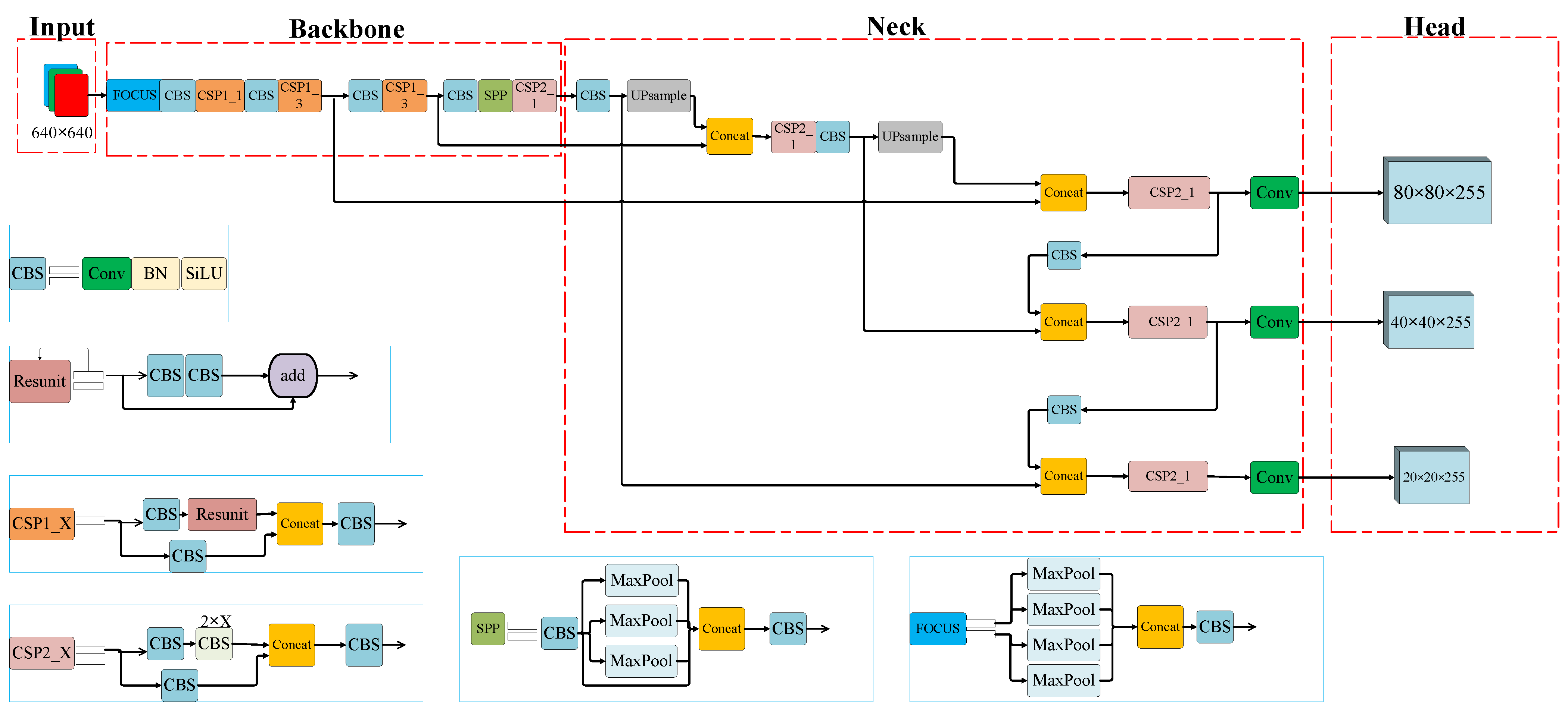
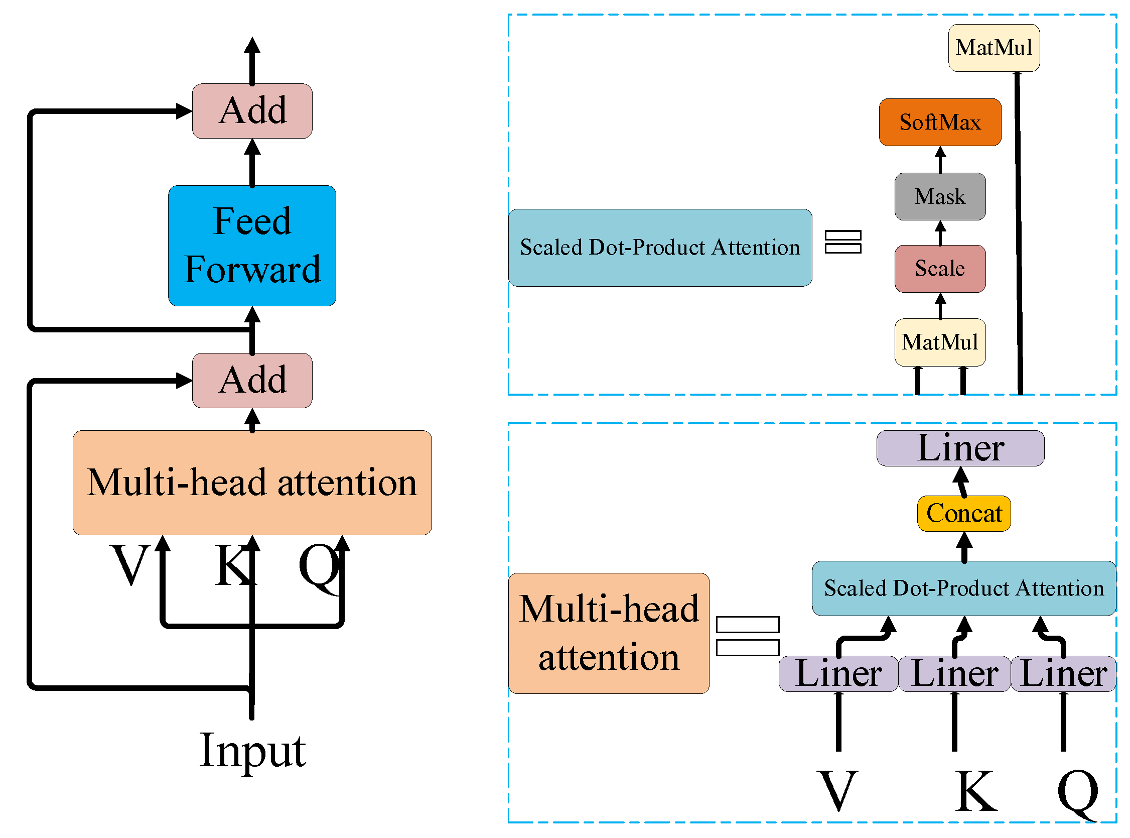
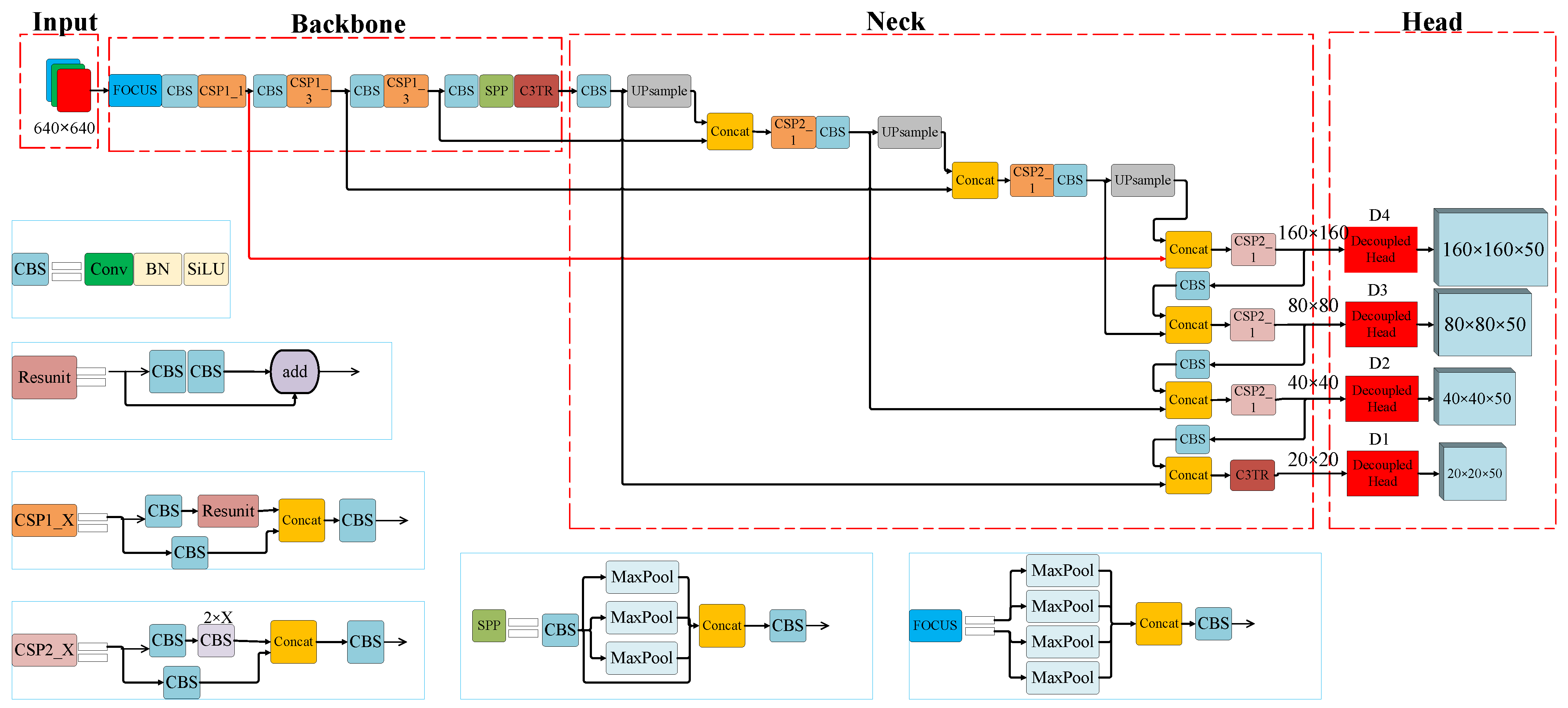
- Replacing the last layer of the ‘Conv + Batch Normalization + SiLU’ (CBS) structure in the YOLOv5s backbone with a transformer self-attention module (T in the YOLOv5-TDHSA‘s name), and also adding a similar module to the last layer of its neck, so that the image information can be used more comprehensively;
- 2.
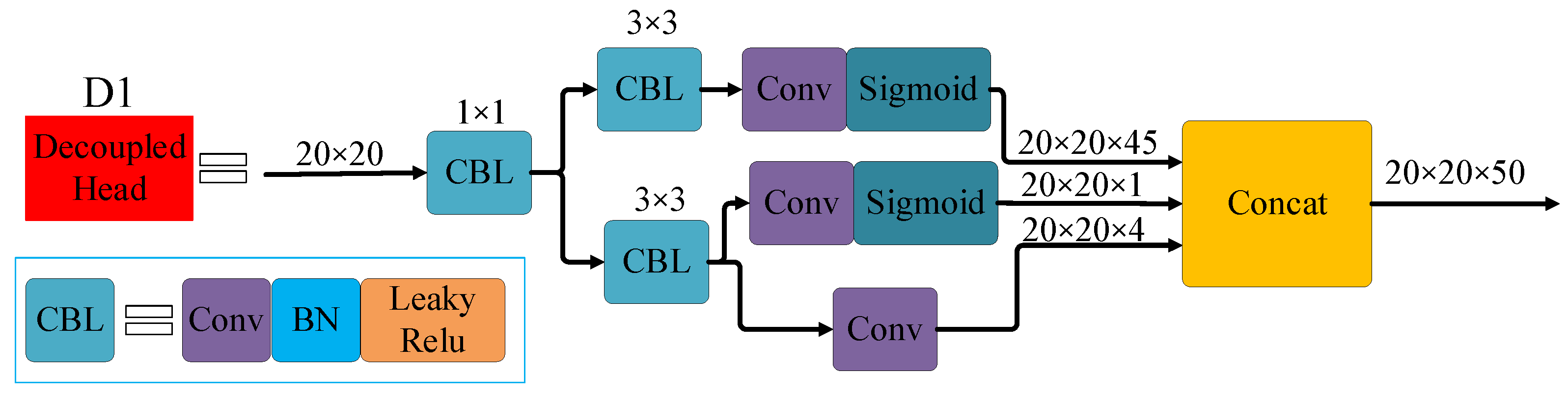
- Replacing the YOLOv5s coupled head with a decoupled head (DH in the both models’ names) so as to increase the detection accuracy and speed up the convergence;
- 3.
- Adding a small-object detection layer (S in the YOLOv5-TDHSA‘s name) and an adaptive anchor (A in the YOLOv5-TDHSA‘s name) to the YOLOv5s neck to improve the detection of small objects.
2. Background
2.1. Attention Mechanisms
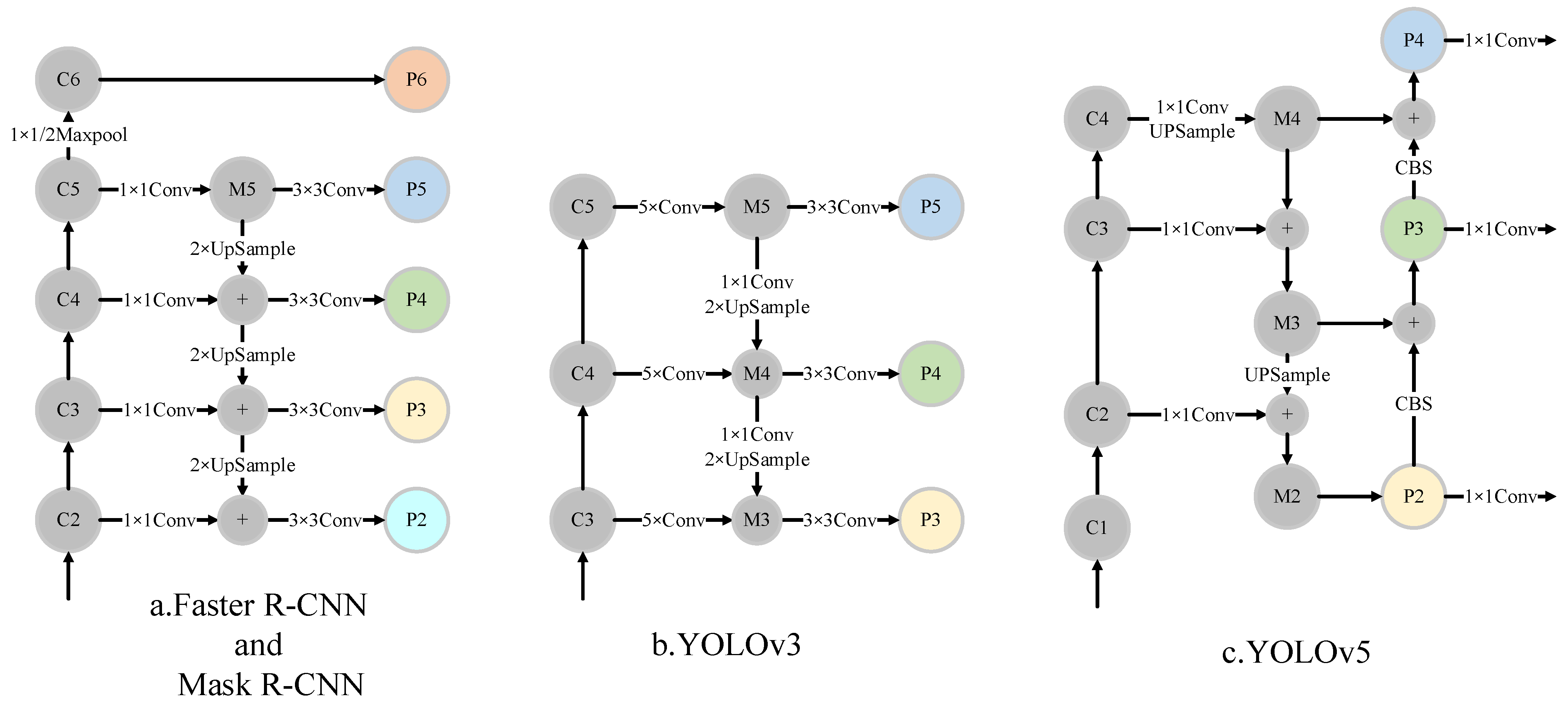
2.2. Multi-Scale Feature Fusion
2.3. Detector Head
3. Related Work
3.1. Two-Stage Object Detection Models
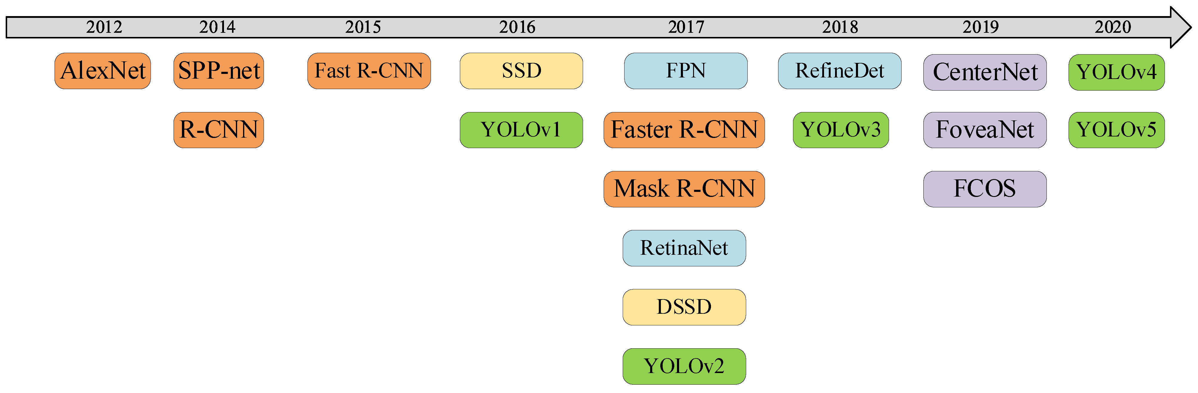
3.2. One-Stage Object Detection Models
3.2.1. YOLO
3.2.2. SSD
4. Proposed Improvements to YOLOv5s
4.1. Transformer Self-Attention Mechanism
4.2. Decoupled Head
4.3. Small-Object Detection Layer and Adaptive Anchor
5. Experiments
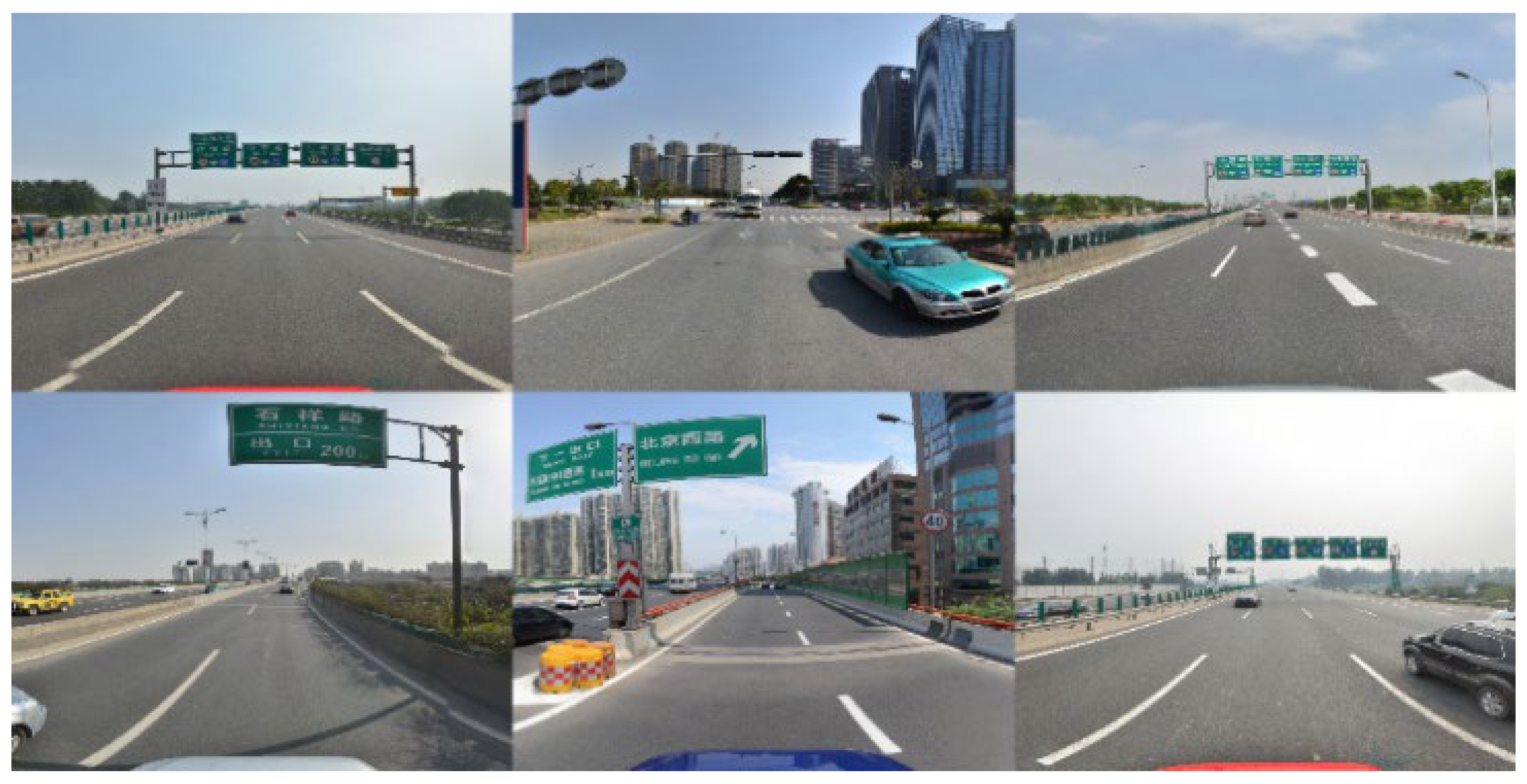
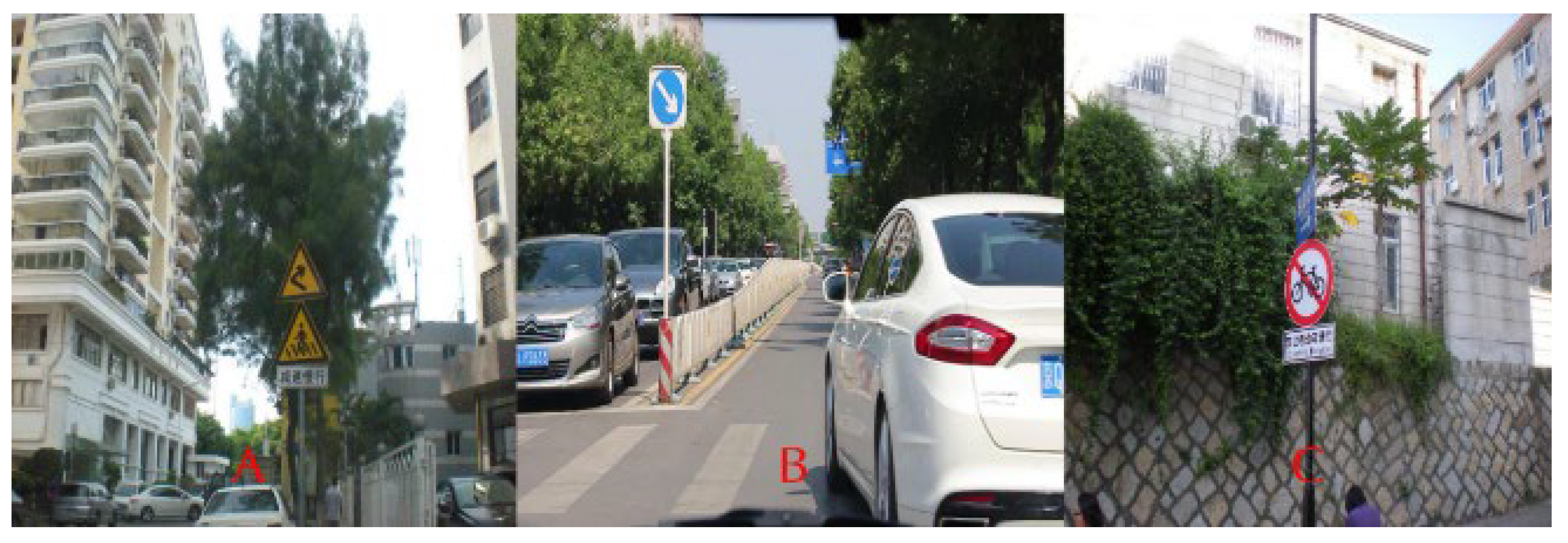
5.1. Datasets
5.2. Experimental Environment
5.3. Evaluation Metrics
5.4. Results
6. Discussion
7. Conclusions
Author Contributions
Funding
Data Availability Statement
Conflicts of Interest
References
- Saadna, Y.; Behloul, A. An overview of traffic sign detection and classification methods. Int. J. Multimed. Inf. Retr. 2017, 6, 193–210. [Google Scholar] [CrossRef]
- Yıldız, G.; Dizdaroğlu, B. Traffic Sign Detection via Color and Shape-Based Approach. Proceedings of 2019 1st International Informatics and Software Engineering Conference (UBMYK), Ankara, Turkey, 6–7 November 2019; pp. 1–5. [Google Scholar]
- Shen, X.; Liu, J.; Zhao, H.; Liu, X.; Zhang, B. Research on Multi-Target Recognition Algorithm of Pipeline Magnetic Flux Leakage Signal Based on Improved Cascade RCNN. Proceedings of 2021 3rd International Conference on Industrial Artificial Intelligence (IAI), Shenyang, China, 8–11 November 2021; pp. 1–6. [Google Scholar]
- Wang, X.; Wang, S.; Cao, J.; Wang, Y. Data-driven based tiny-YOLOv3 method for front vehicle detection inducing SPP-net. IEEE Access 2020, 8, 110227–110236. [Google Scholar] [CrossRef]
- Rani, S.; Ghai, D.; Kumar, S. Object detection and recognition using contour based edge detection and fast R-CNN. Multimed. Tools Appl. 2022, 81, 42183–42207. [Google Scholar] [CrossRef]
- Ren, S.; He, K.; Girshick, R.; Sun, J. Faster R-CNN: Towards Real-Time Object Detection with Region Proposal Networks. IEEE Trans. Pat. Analys. Mach. Intell. 2017, 39, 1137–1149. [Google Scholar] [CrossRef] [PubMed]
- Fan, J.; Huo, T.; Li, X. A Review of One-Stage Detection Algorithms in Autonomous Driving. Proceedings of 2020 4th CAA International Conference on Vehicular Control and Intelligence (CVCI), Hangzhou, China, 18–20 December 2020; pp. 210–214. [Google Scholar]
- Redmon, J.; Divvala, S.; Girshick, R.; Farhadi, A. You Only Look Once: Unified, Real-Time Object Detection. In Proceedings of Proceedings of the IEEE Conference on Computer Vision and Pattern Recognition, San Juan, PR, USA, 17–19 June 1997; pp. 779–788. [Google Scholar]
- Redmon, J.; Farhadi, A. YOLO9000: Better, Faster, Stronger. In Proceedings of Proceedings of the IEEE Conference on Computer Vision and Pattern Recognition, San Juan, PR, USA, 17–19 June 1997; pp. 7263–7271. [Google Scholar]
- Lv, N.; Xiao, J.; Qiao, Y. Object Detection Algorithm for Surface Defects Based on a Novel YOLOv3 Model. Processes 2022, 10, 701. [Google Scholar] [CrossRef]
- Bochkovskiy, A.; Wang, C.-Y.; Liao, H.-Y.M. Yolov4: Optimal speed and accuracy of object detection. arXiv 2020, arXiv:2004.10934. [Google Scholar]
- Ma, W.; Zhou, T.; Qin, J.; Zhou, Q.; Cai, Z. Joint-attention feature fusion network and dual-adaptive NMS for object detection. Knowl. Based Syst. 2022, 241, 108213. [Google Scholar] [CrossRef]
- Niu, Z.; Zhong, G.; Yu, H. A review on the attention mechanism of deep learning. Neurocomputing 2021, 452, 48–62. [Google Scholar] [CrossRef]
- Hu, J.; Shen, L.; Sun, G. Squeeze-And-Excitation Networks. In Proceedings of the IEEE Conference on Computer Vision and Pattern Recognition, San Juan, PR, USA, 17–19 June 1997; pp. 7132–7141. [Google Scholar]
- Woo, S.; Park, J.; Lee, J.-Y.; Kweon, I.S. Cbam: Convolutional block attention module. In Proceedings of the European Conference on Computer Vision (ECCV), Glasgow, UK, 23–28 August 2020; pp. 3–19. [Google Scholar]
- Liang, H.; Zhou, H.; Zhang, Q.; Wu, T. Object Detection Algorithm Based on Context Information and Self-Attention Mechanism. Symmetry 2022, 14, 904. [Google Scholar] [CrossRef]
- Lou, Y.; Ye, X.; Li, M.; Li, H.; Chen, X.; Yang, X.; Liu, X. Object Detection Model of Cucumber Leaf Disease Based on Improved FPN. Proceedings of 2022 IEEE 6th Advanced Information Technology, Electronic and Automation Control Conference (IAEAC), Beijing, China, 3–5 October 2022; pp. 743–750. [Google Scholar]
- He, K.; Gkioxari, G.; Dollár, P.; Girshick, R. Mask R-Cnn. In Proceedings of the IEEE International Conference on Computer Vision, Venice, Italy, 22–29 October 2017; pp. 2961–2969. [Google Scholar]
- Liu, S.; Qi, L.; Qin, H.; Shi, J.; Jia, J. Path Aggregation Network for Instance Segmentation. arXiv 2018, arXiv:1803.01534. [Google Scholar]
- Zheng, Z.; Wang, P.; Liu, W.; Li, J.; Ye, R.; Ren, D. Distance-IoU loss: Faster and better learning for bounding box regression. Proc. Proc. AAAI Conf. Artif. Intell. 2020, 34, 12993–13000. [Google Scholar] [CrossRef]
- Zou, Z.; Shi, Z.; Guo, Y.; Ye, J. Object detection in 20 years: A survey. arXiv 2019, arXiv:1905.05055. [Google Scholar] [CrossRef]
- Xiao, Y.; Tian, Z.; Yu, J.; Zhang, Y.; Liu, S.; Du, S.; Lan, X. A review of object detection based on deep learning. Multimed. Tools Appl. 2020, 79, 23729–23791. [Google Scholar] [CrossRef]
- Dixit, U.D.; Shirdhonkar, M.; Sinha, G. Automatic logo detection from document image using HOG features. Multimed. Tools Appl. 2022, 82, 863–878. [Google Scholar] [CrossRef]
- Kim, J.; Lee, K.; Lee, D.; Jhin, S.Y.; Park, N. DPM: A novel training method for physics-informed neural networks in extrapolation. Proc. Proc. AAAI Conf. Artif. Intell. 2021, 35, 8146–8154. [Google Scholar] [CrossRef]
- Krizhevsky, A.; Sutskever, I.; Hinton, G.E. Imagenet classification with deep convolutional neural networks. Commun. ACM 2017, 60, 84–90. [Google Scholar] [CrossRef]
- Niepceron, B.; Grassia, F.; Moh, A.N.S. Brain Tumor Detection Using Selective Search and Pulse-Coupled Neural Network Feature Extraction. Comput. Inform. 2022, 41, 253–270. [Google Scholar] [CrossRef]
- Du, L.; Zhang, R.; Wang, X. Overview of Two-Stage Object Detection Algorithms. Proc. J. Phys. Conf. Ser. 2020, 1544, 012033. [Google Scholar] [CrossRef]
- Jiang, P.; Ergu, D.; Liu, F.; Cai, Y.; Ma, B. A Review of Yolo algorithm developments. Procedia Comput. Sci. 2022, 199, 1066–1073. [Google Scholar] [CrossRef]
- Bouabid, S.; Delaitre, V. Mixup regularization for region proposal based object detectors. arXiv 2020, arXiv:2003.02065. [Google Scholar]
- Chen, Y.; Wang, J.; Dong, Z.; Yang, Y.; Luo, Q.; Gao, M. An Attention based YOLOv5 Network for Small Traffic Sign Recognition. Proceedings of 2022 IEEE 31st International Symposium on Industrial Electronics (ISIE), Anchorage, AK, USA, 1–3 June 2022; pp. 1158–1164. [Google Scholar]
- Liu, X.; Jiang, X.; Hu, H.; Ding, R.; Li, H.; Da, C. Traffic Sign Recognition Algorithm Based on Improved YOLOv5s. Proceedings of 2021 International Conference on Control, Automation and Information Sciences (ICCAIS), Xi’an, China, 14–17 October 2021; pp. 980–985. [Google Scholar]
- Chen, X. Traffic Lights Detection Method Based on the Improved YOLOv5 Network. Proceedings of 2022 IEEE 4th International Conference on Civil Aviation Safety and Information Technology (ICCASIT), Dali, China, 12–14 October 2022; pp. 1111–1114. [Google Scholar]
- Chen, Z.; Guo, H.; Yang, J.; Jiao, H.; Feng, Z.; Chen, L.; Gao, T. Fast vehicle detection algorithm in traffic scene based on improved SSD. Measurement 2022, 201, 111655. [Google Scholar] [CrossRef]
- Vaswani, A.; Shazeer, N.; Parmar, N.; Uszkoreit, J.; Jones, L.; Gomez, A.N.; Kaiser, Ł.; Polosukhin, I. Attention is all you need. Proceedings of Advances in Neural Information Processing Systems 30 (NIPS 2017), Long Beach, CA, USA, 4–9 December 2017. [Google Scholar]
- Ge, Z.; Liu, S.; Wang, F.; Li, Z.; Sun, J. Yolox: Exceeding yolo series in 2021. arXiv 2021, arXiv:2107.08430. [Google Scholar]
- Ballantyne, G.H. Review of sigmoid volvulus. Dis. Colon Rectum 1982, 25, 823–830. [Google Scholar] [CrossRef] [PubMed]
- Wang, J.; Chen, Y.; Gao, M.; Dong, Z. Improved YOLOv5 network for real-time multi-scale traffic sign detection. arXiv 2021, arXiv:2112.08782. [Google Scholar] [CrossRef]
- Zhu, Z.; Liang, D.; Zhang, S.; Huang, X.; Li, B.; Hu, S. Traffic-Sign Detection and Classification in the Wild. In Proceedings of the IEEE Conference on Computer Vision and Pattern Recognition, San Juan, PR, USA, 17–19 June 1997; pp. 2110–2118. [Google Scholar]
- Chen, J.; Jia, K.; Chen, W.; Lv, Z.; Zhang, R. A real-time and high-precision method for small traffic-signs recognition. Neural Comput. Appl. 2022, 34, 2233–2245. [Google Scholar] [CrossRef]
- Zhang, J.; Zou, X.; Kuang, L.-D.; Wang, J.; Sherratt, R.S.; Yu, X. CCTSDB 2021: A more comprehensive traffic sign detection benchmark. Hum. Cent. Comput. Inf. Sci. 2022, 12, 23. [Google Scholar]
- Zhang, J.; Huang, M.; Jin, X.; Li, X. A real-time Chinese traffic sign detection algorithm based on modified YOLOv2. Algorithms 2017, 10, 127. [Google Scholar] [CrossRef]
- Zhang, J.; Jin, X.; Sun, J.; Wang, J.; Sangaiah, A.K. Spatial and semantic convolutional features for robust visual object tracking. Multimed. Tools Appl. 2020, 79, 15095–15115. [Google Scholar] [CrossRef]
- Friedman, M. The use of ranks to avoid the assumption of normality implicit in the analysis of variance. J. Am. Stat. Assoc. 1937, 32, 675–701. [Google Scholar] [CrossRef]
- Friedman, M. A comparison of alternative tests of significance for the problem of m rankings. Ann. Math. Stat. 1940, 11, 86–92. [Google Scholar] [CrossRef]
- Dunn, O.J. Multiple Comparisons among Means. J. Am. Stat. Assoc. 1961, 56, 52–64. [Google Scholar] [CrossRef]
- Lin, Y.; Hu, Q.; Liu, J.; Li, J.; Wu, X. Streaming feature selection for multilabel learning based on fuzzy mutual information. IEEE Trans. Fuzzy Syst. 2017, 25, 1491–1507. [Google Scholar] [CrossRef]
- Iman, R.L.; Davenport, J.M. Approximations of the critical region of the fbietkan statistic. Commun. Stat. Theory Methods 1980, 9, 571–595. [Google Scholar] [CrossRef]
- Demšar, J. Statistical Comparisons of Classifiers over Multiple Data Sets. J. Mach. Learn. Res. 2006, 7, 1–30. [Google Scholar]


| TT100K Dataset | CCTSDB2021 Dataset | |
|---|---|---|
| Training set | 13,908 labels | 1935 labels |
| Validation set | 4636 labels | 645 labels |
| Test set | 4636 labels | 645 labels |
| Component | Name/Value |
|---|---|
| Operating system | Windows 10 |
| CPU | Intel (R) Core (TM) i7-10,700 |
| GPU | GeForce RTX3090 |
| Video memory | 24 GB |
| Training acceleration | CUDA 11.1 |
| Deep learning framework for training | PyTorch 1.8.1 |
| Input image size | 640 × 640 pixels |
| Initial learning rate | 0.01 |
| Final learning rate | 0.1 |
| Training batch size | 32 |
| Model | Size (MB) | Number of Parameters (Million) |
|---|---|---|
| Faster R-CNN | 360.0 | 28.469 |
| YOLOv4-Tiny | 22.4 | 6.057 |
| YOLOv5n | 3.6 | 1.767 |
| YOLOv5s | 13.7 | 7.068 |
| YOLOv5-DH | 22.8 | 11.070 |
| YOLOv5-TDHSA | 24.8 | 12.224 |
| Dataset | Faster R-CNN | YOLOv4-Tiny | YOLOv5n | YOLOv5s | YOLOv5- DH | YOLOv5- TDHSA |
|---|---|---|---|---|---|---|
| TT100K | 47 h | 37.5 h | 30 h | 32 h | 33 h | 35 h |
| CCTSDB 2021 | 8.5 h | 4 h | 0.8 h | 1 h | 2 h | 2.5 h |
| Experiment 1 | Experiment 2 | Experiment 3 | Experiment 4 | Experiment 5 | |
|---|---|---|---|---|---|
| mAP (%) | 52.9 | 53.6 | 54.1 | 53.4 | 52.6 |
| F1 score | 0.576 | 0.581 | 0.586 | 0.579 | 0.575 |
| Experiment 1 | Experiment 2 | Experiment 3 | Experiment 4 | Experiment 5 | |
|---|---|---|---|---|---|
| mAP (%) | 57.7 | 62.8 | 63.1 | 64.6 | 63.2 |
| F1 score | 0.608 | 0.672 | 0.655 | 0.654 | 0.675 |
| Experiment 1 | Experiment 2 | Experiment 3 | Experiment 4 | Experiment 5 | |
|---|---|---|---|---|---|
| mAP (%) | 66.0 | 66.2 | 65.1 | 66.3 | 66.6 |
| F1 score | 0.651 | 0.645 | 0.639 | 0.646 | 0.641 |
| Experiment 1 | Experiment 2 | Experiment 3 | Experiment 4 | Experiment 5 | |
|---|---|---|---|---|---|
| mAP (%) | 74.5 | 75.6 | 75.2 | 75.3 | 75.1 |
| F1 score | 0.728 | 0.741 | 0.740 | 0.730 | 0.728 |
| Experiment 1 | Experiment 2 | Experiment 3 | Experiment 4 | Experiment 5 | |
|---|---|---|---|---|---|
| mAP (%) | 77.2 | 78.3 | 77.6 | 78.5 | 78.1 |
| F1 score | 0.762 | 0.771 | 0.762 | 0.772 | 0.769 |
| Experiment 1 | Experiment 2 | Experiment 3 | Experiment 4 | Experiment 5 | |
|---|---|---|---|---|---|
| mAP (%) | 83.3 | 83.5 | 82.6 | 83.3 | 84.2 |
| F1 score | 0.819 | 0.811 | 0.797 | 0.810 | 0.816 |
| Model | F1Score | mAP (%) | Processing Speed (fps) |
|---|---|---|---|
| Faster R-CNN | 0.579 | 53.3 | 40 |
| YOLOv4-Tiny | 0.653 | 62.3 | 160 |
| YOLOv5n | 0.644 | 66.0 | 111 |
| YOLOv5s | 0.733 | 75.1 | 100 |
| YOLOv5-DH | 0.767 | 77.9 | 84 |
| YOLOv5-TDHSA | 0.811 | 83.4 | 77 |
| Experiment 1 | Experiment 2 | Experiment 3 | Experiment 4 | Experiment 5 | |
|---|---|---|---|---|---|
| mAP (%) | 61.9 | 48.7 | 45.7 | 46.0 | 61.1 |
| F1 score | 0.65 | 0.62 | 0.59 | 0.61 | 0.65 |
| Experiment 1 | Experiment 2 | Experiment 3 | Experiment 4 | Experiment 5 | |
|---|---|---|---|---|---|
| mAP (%) | 62.6 | 64.2 | 53.7 | 62.3 | 64.7 |
| F1 score | 0.66 | 0.68 | 0.62 | 0.65 | 0.67 |
| Experiment 1 | Experiment 2 | Experiment 3 | Experiment 4 | Experiment 5 | |
|---|---|---|---|---|---|
| mAP (%) | 68.7 | 72.5 | 54.8 | 60.7 | 71.3 |
| F1 score | 0.72 | 0.72 | 0.60 | 0.63 | 0.74 |
| Experiment 1 | Experiment 2 | Experiment 3 | Experiment 4 | Experiment 5 | |
|---|---|---|---|---|---|
| mAP (%) | 64.7 | 70.2 | 58.9 | 68.5 | 73.7 |
| F1 score | 0.70 | 0.72 | 0.63 | 0.69 | 0.76 |
| Experiment 1 | Experiment 2 | Experiment 3 | Experiment 4 | Experiment 5 | |
|---|---|---|---|---|---|
| mAP (%) | 71.9 | 67.6 | 62.2 | 65.2 | 73.8 |
| F1 score | 0.71 | 0.70 | 0.68 | 0.68 | 0.76 |
| Experiment 1 | Experiment 2 | Experiment 3 | Experiment 4 | Experiment 5 | |
|---|---|---|---|---|---|
| mAP (%) | 69.1 | 73.4 | 62.1 | 69.7 | 74.7 |
| F1 score | 0.73 | 0.76 | 0.66 | 0.67 | 0.76 |
| Model | F1Score | mAP (%) | Processing Speed (fps) |
|---|---|---|---|
| Faster R-CNN | 0.62 | 52.7 | 28 |
| YOLOv4-Tiny | 0.66 | 61.5 | 162 |
| YOLOv5n | 0.68 | 65.6 | 83 |
| YOLOv5s | 0.70 | 67.2 | 77 |
| YOLOv5-DH | 0.71 | 68.1 | 70 |
| YOLOv5-TDHSA | 0.72 | 69.8 | 66 |
Disclaimer/Publisher’s Note: The statements, opinions and data contained in all publications are solely those of the individual author(s) and contributor(s) and not of MDPI and/or the editor(s). MDPI and/or the editor(s) disclaim responsibility for any injury to people or property resulting from any ideas, methods, instructions or products referred to in the content. |
© 2023 by the authors. Licensee MDPI, Basel, Switzerland. This article is an open access article distributed under the terms and conditions of the Creative Commons Attribution (CC BY) license (https://creativecommons.org/licenses/by/4.0/).
Share and Cite
Bai, W.; Zhao, J.; Dai, C.; Zhang, H.; Zhao, L.; Ji, Z.; Ganchev, I. Two Novel Models for Traffic Sign Detection Based on YOLOv5s. Axioms 2023, 12, 160. https://doi.org/10.3390/axioms12020160
Bai W, Zhao J, Dai C, Zhang H, Zhao L, Ji Z, Ganchev I. Two Novel Models for Traffic Sign Detection Based on YOLOv5s. Axioms. 2023; 12(2):160. https://doi.org/10.3390/axioms12020160
Chicago/Turabian StyleBai, Wei, Jingyi Zhao, Chenxu Dai, Haiyang Zhang, Li Zhao, Zhanlin Ji, and Ivan Ganchev. 2023. "Two Novel Models for Traffic Sign Detection Based on YOLOv5s" Axioms 12, no. 2: 160. https://doi.org/10.3390/axioms12020160