Article

A Study of The Stochastic Burgers’ Equation Using The Dynamical Orthogonal Method

1
Engineering Mathematics and Physics Department, Engineering Faculty, Cairo University, Giza 12613, Egypt
2
Department of Information Technology, Faculty of Computing and Information Technology, King Abdulaziz University, Jeddah 80221, Saudi Arabia
*
Author to whom correspondence should be addressed.
Axioms 2023, 12(2), 152; https://doi.org/10.3390/axioms12020152
Submission received: 24 December 2022 / Revised: 27 January 2023 / Accepted: 31 January 2023 / Published: 1 February 2023
(This article belongs to the Special Issue Advances in Numerical Analysis and Scientific Computing)

Abstract

:
In the current work, the stochastic Burgers’ equation is studied using the Dynamically Orthogonal (DO) method. The DO presents a low-dimensional representation for the stochastic fields. Unlike many other methods, it has a time-dependent property on both the spatial basis and stochastic coefficients, with flexible representation especially in the strongly transient and nonstationary problems. We consider a computational study and application of the DO method and compare it with the Polynomial Chaos (PC) method. For comparison, both the stochastic viscous and inviscid Burgers’ equations are considered. A hybrid approach, combining the DO and PC is proposed in case of deterministic initial conditions to overcome the singularities that occur in the DO method. The results are verified with the stochastic collocation method. Overall, we observe that the DO method has a higher rate of convergence as the number of modes increases. The DO method is found to be more efficient than PC for the same level of accuracy, especially for the case of high-dimensional parametric spaces. The inviscid Burgers’ equation is analyzed to study the shock wave formation when using the DO after suitable handling of the convective term. The results show that the sinusoidal wave shape is distorted and sharpened as the time evolves till the shock wave occurs.

1. Introduction

Recently, there has been a compelling need to quantify uncertainties of parameters in physical and mathematical problems in a probabilistic framework. This includes cases that can be characterized by stochastic partial differential equations (SPDEs). Theses equations appear in many application fields, for example, solid mechanics, random vibrations, fluid dynamics [1,2,3], propagation of waves through random media [4,5,6], and finance [7]. Stochastic forcing, uncertainties in one or more physical parameters, and initial and/or boundary values, among others, are contributing to stochasticity in many disciplines.
Burgers’ equation is one of many important models that appear in many applications specially in fluid mechanics. When considering the stochastic effects added to Burgers’ equation, it will be extended to study some real-life applications such as the flow turbulence. There are various techniques that can be used to study and analyze such stochastic models. The Monte Carlo (MC) simulation [8,9,10] is one of the most practical methods, using a sequence of random numbers to handle these problems and get useful statistical properties. To attain a certain accuracy level, a sufficient number of samples are required. More studies have been applied to improve the MC efficiency such as sequential Monte Carlo methods [11,12] and the Error Subspace Statistical Estimation (ESSE) [13,14]. The MC-based techniques still have a relatively low rate of convergence and/or do not work efficiently for the general case [15].
Order-reduction techniques have been employed to simplify and analyze high-dimensional complicated systems relative to several scientific and engineering problems. Hence, they provide lower complexity for the original SPDE model. One of these approaches is the Proper Orthogonal Decomposition (POD) [16], which is based on the statistical technique of Karhunen-Loeve (KL) expansion. The main drawback is that the spatial basis of the POD method is selected a priori, which means that it may be unable to describe some problems, such as transient fluid flows, which are highly time-dependent and make the basis used irrelevant as time evolves.
Ghanem and Spanos [17] introduced an important and widely used approach known as the Polynomial Chaos (PC) expansion, which is based on Wiener’s theory on polynomial chaos [18]. The main drawback is that the PC suffers from problems relying on long time dependence, although it is well known that the PC method shows fast convergence rates for Gaussian processes. Other types of processes may have slower convergence rates in addition to solution deterioration with time evolution. The generalized PC expansion (gPC) introduced by Xiu and Karniadakis [19,20] uses different basis functions for different types of problems and is employed to increase the rate of convergence and to improve the efficiency of a wide range of nonlinear applications. The Probabilistic Collocation Method (PCM) [21] is an efficient version derived from PC that provides a smooth solution in parametric spaces and gives fast convergence rates as the order of the expansion increases [22,23].
The PC can also be extended to analyze the stochastic differential equations (SDEs) which are derived by or include white noise. The Wiener chaos expansion (WCE) and the Wiener-Hermite expansion (WHE) are common techniques used for analyzing SDEs [24]. The fractional-order version of the WHE was recently developed for the case of fractional Brownian motion [25].
In the current study, we shall focus on analyzing Burgers’ model with stochastic forcing. The stochastic Burgers’ model is common in studying flow turbulence and in general the propagation of randomness and nonlinear waves in the undispersive media [24]. The same type of nonlinearity of Burgers’ equation exists as in Navier-Stokes equations. Results obtained from solving the 1D stochastic Burgers’ equation are similar to experimental results of the 3D real turbulence problems.
Dynamical Orthogonal (DO) decomposition is introduced in [26,27] as one of the reduced-order techniques in which the solution is approximated in a generalized KL expansion, i.e.,
u x , t ; ω = u ¯ x , t + i = 1 N u i x , t Y i t ; ω ,
where x is an n-dimension space vector, t > 0 is the time, ω is the output of a random experiment, N represents the number of approximating modes,   u ¯ x , t is the mean field, and u i x , t   ; i = 0   t o   N , are orthonormal time-dependent fields in the spatial domain. The stochastic processes Y i t ; ω are usually considered to be with zero mean without loss of generality. Both spatial basis and the stochastic coefficients have a time dependency. As a result, the above KL representation is particularly flexible when it comes to represent nonstationary, highly transient responses. On the other hand, the same property adopts a redundant representation. To overcome this redundancy in both stochastic coefficients and spatial basis, a natural constraint is imposed, called the dynamical orthogonal condition [26]. By means of this condition, the DO components, i.e., u i x , t , Y i t ; ω and u ¯ x , t , can be derived.
From a computational viewpoint, the uncertainty evolution using DO decomposition is accomplished by determining a set of N + 1 deterministic PDEs that describe the mean field evolution u ¯ x , t and the basis u i x , t coupled with N (ordinary) SDEs that describe the evolution of stochastic coefficients Y i t ; ω . The DO equations reach a singularity at very low levels of uncertainty when the modes develop independently. Therefore, this may generate a numerical issue since the computations include ratios of small moment quantities, particularly in problems where deterministic initial conditions are included. The initialization of the random space is another issue that arises when starting with deterministic initial conditions.
To address these issues, a hybrid approach is introduced in [28] that avoids the singularity that occurs in the covariance matrix. This hybrid approach was formulated by integrating the PC with the DO method. Firstly, the PC is used in solving the SPDE up to a certain time until guaranteeing the development of stochasticity. Next, the DO approach is used to continue the solution with time evolution. As part of this strategy, the KL expansion is employed to give a collection of modes that are used for initializing the stochastic coefficients.
In the current work, we study the stochastic Burgers’ model using the DO method and compare it with the PC from different sides including error behavior, effect of switching time, and the number of modes and their effect on solution accuracy. Moreover, the error between DO components and the growth of eigenvalues are computed. The DO behavior for the case of inviscid Burgers’ equation and shock wave formation is also analyzed in the current work. Suitable known techniques, such as upwind techniques [29], are combined with the DO method to analyze the shock formation in the presence of random coefficients.
The paper is structured as follows: In Section 2, we provide a brief overview of the construction of the DO representation, the evolution equations, and their numerical solution. A hybrid approach combining the DO and PC is presented. In Section 3, the performance of the DO and PCM methods are compared by analyzing the stochastic viscous and inviscid Burgers’ equations. In Section 4, we study shock wave formation via inviscid Burgers’ equation. In Section 5, we present the conclusions.

2. Methodology

Consider the probability space ( Ω   ,   F , P ) where the sample space Ω contains all the elementary events ω   .   F is the σ -algebra of the subsets of Ω , and P is the probability measure. The random field will be defined for all measurable maps with the form u x , t , ω . The mean value operator of u is formulated as follows:
u ¯ x , t = E u x , t ; ω = Ω u x , t ; ω d P ω .
The set of continuous random fields that are square integrable, i.e., D E [ u x , t ; ω T u x , t ; ω ]   d x < , where the transpose of u x , t ; ω is u x , t ; ω T for all t   ϵ   T ; where D is the domain and T is the time interval. The covariance operator, between two random fields u x , t ; ω and q x , t ; ω , has the bi-linear form:
C u ,   q x , y = E u x , t ; ω u ¯ x , t T q y , τ ; ω q ¯ y , τ ,
where x , y   belong   to   the   spatial   domain   D ,   t , τ   T , and forms a Hilbert space H [4,30]. For the random u x , t ; ω the projection operator to subspace spanned by the orthonormal basis Q = s j x , t ; ω j = 1 m is defined as follows:
Q u x , t ; ω = j = 1 m s j . , t ; ω , u . , t ; ω   s j x , t ; ω .
We define the autocovariance operator for u x , t ; ω in the case τ = t as follows:
C u , u x , y = E u x , t ; ω u ¯ x , t T u y , t ; ω u ¯ y , t ,
where x , y D ,   t   T   . Then, we define the integral operator at a given time t which depends on the autocovariance operator as follows:
Ι C   ϕ = D C u , u x , y   ϕ x , t d x ; ϕ L 2 .  
and it is a positive operator, compact and self-adjoint in the Hilbert space H of a deterministic, square-integrable, and continuous field L 2 [16,31].
In the current work, we shall consider the following evolution SPDE:
u x , t ; ω t = L u x , t ; ω , ω ;   x D ,   t T ,   ω Ω ,
where L is the differential operator, generally nonlinear. The system initial condition at time t 0 is given by the random field:
u x , t 0 ;   ω = u 0 x ; ω .
and the boundary conditions take the form:
B u ξ , t ; ω = h ξ , t ; ω ;   ξ D ,
where B is a differential linear operator and D is the boundary of domain D in R n and n = 1 ,   2 or 3 .

2.1. DO Method

For every random field u x , t , ω L 2 , the KL expansion [29,30] at time t can be written as:
u x , t ; ω = u ¯ x , t + i = 1 Y i t ; ω   u i x , t ,
where u i x , t are the eigenfunctions and Y i t ; ω are stochastic processes. We can obtain the eigenfunctions and eigenvalues of the covariance matrix C of u i x , t by solving:
D C u ,   u x , y   u i x , t   d x = λ i   u i y , t ,
where u i are orthonormal eigenfunctions, i.e., u i , u j = δ i j   . Then, we can approximate the random field u x , t , ω by a finite N-modes series expansion as:
u x , t , ω = u ¯ x , t + i = 1 N Y i t ; ω   u i x , t .
The stochastic subspace V s = s p a n u i x , t i = 1 N is defined as the space spanned by the eigenfunctions of the largest N eigenvalues. It is worth noting that the spatial basis u i x , t and stochastic coefficients Y i t ; ω are recognized to have a time-dependent nature, and they change in relation to system dynamics.
The mean component u ¯ x , t , the orthogonal basis u i x , t i = 1 N , and the stochastic coefficients Y i t ; ω i = 1 N are all time-dependent and they are varyingly redundant. The main cause of redundancy arises from the uncertainty of evolution. In order to solve this redundancy, we can limit the basis u i x , t i = 1 N evolution to be only orthogonal to the space V s by imposing additional constraints. For example, we can apply the following orthogonality constraint:
d V s d t   V s u j x , t t ,   u i x , t = 0 ;   i , j = 1 , , N .
This constraint is known as the dynamical orthogonal condition [26,32]. This is also equivalent to preserving the basis u i x , t i = 1 N orthogonality for all times since:
t u j . , t , u i . , t = u j x , t t ,   u i x , t + u j x , t , u i x , t t .
The DO expansion is used to obtain a set of independent equations characterizing all deterministic and stochastic quantities. Using DO, we will be able to reduce the SPDE to a set of N + 1 deterministic PDEs for u ¯ x , t and u i x , t i = 1 N coupled with N ordinary differential equations in the stochastic coefficients Y i x , t i = 1 N .
Under the DO representation, the main SPDE (6)–(8) can be reformulated into the following system of equations [26]:
u ¯ x , t t = E   L u x , t ; ω ; ω .
u i x , t t = V s E L u . , t ; ω ; ω Y j t ; ω   C Y i t Y j t . 1
d Y i t ; ω d t = L u x , t ; ω ; ω E   L u x , t ; ω ; ω , u i x , t ,
where V s F x = F x V s F x = F x F . , u k . , t   u k is the orthogonal complement projection, and C Y i t Y j t = E Y i t ; ω Y j t ; ω is the covariance operator for the stochastic coefficients. The related boundary values are given by:
B u ¯ ξ , t ; ω = E h ξ , t ; ω .
B u i ξ , t = E Y i t ; ω h ξ , t ; ω   C Y i t Y j t . 1
where ξ D and the initial conditions at time t 0 have the form:
u ¯ x , t 0 = u ¯ 0 . E u 0 x ; ω .  
u i x , t 0 = u i 0 x .  
Y i t 0 ; ω = u 0 . ; ω u ¯ 0 . , u i 0 . ,
for i = 1 , , N , and u i 0 x are the eigenfunctions associated with the covariance operator C u , u .

2.2. Numerical Solution

The DO evolution Equations (14)–(16) include numerical integration for both random and physical spaces. We denote the weights and collocation points of the spatial space by x p , w p p = 1 N s and for the random space by ξ j , γ j j = 1 N r . We can use Fourier collocation points for x p ,   p = 1 ,   , N s , and Legendre-Gauss collocation for ξ j ,   j = 1 , ,   N r . To discretize time, explicit procedures can be used such as Euler’s method and 4th-order Runge-Kutta (RK4) method. The inner products included in the KL equations can be evaluated as:
  • The inner product defined in the spatial domain:
p x , t ; ω , q x , t ; ω p = 1 N s p x p , t ; ω   q x p , t ; ω w p .
  • The mean value operator defined in random space:
E p x , t ; ω , q x , t ; ω j = 1 N r p x , t ; ξ j   q x , t ; ξ j γ j .
The evolution equations of the DO representation (14)–(16) can be alternatively reformulated into a matrix form as follows:
u ¯ t = E L u .   u t = p u G C 1 . d Y d t = h .
where:
C i j = E Y i   Y j . h j = L u E L u , u j . , t .   p j = E L u   Y j .   G i j = E L u   Y j , u i .
Practically, in several cases, the initial conditions are deterministic, and the stochasticity emanates from other causes such as random forcing and random coefficients. In this case, the stochastic basis Y i will be initially zero, and hence the covariance matrix for the stochastic coefficients C = E Y T Y will be singular. For this reason, a hybrid approach, combining the PCM and DO methods, is proposed to overcome this problem [28]. We can start the computation with the PCM method to allow the development of randomness up to a certain converting (switching) time t s , then transform to the DO method and use KL expansion to initialize the DO components u ¯   , Y i and u i [33,34].

3. Demonstrating Examples

In this section, we shall consider using the DO and PCM-DO methods to analyze Burgers’ viscous and inviscid models with random parameters. For the numerical computations, we shall consider the following parameters:
t = 0.001 , t f = 5 ,   N s = 128 ,   N r = 64 ,   σ = 1 , v ¯ = 1 ,
where N s refers to the number of collocation points in the physical domain and N r is the number of points in the random domain. The physical domain is discretized using the Fourier collocation points, while the random space is discretized using the Legendre-Gauss collocation. The RK4 method is employed for the time-integrator. At t = 0 , the stochastic variations are zero; i.e., Y i and u i cannot be declared. The DO representation could not be initialized at t = 0 . Therefore, we start the simulation at t = t to avoid the singularity issue due to the presence of deterministic (nonrandom) initial conditions. The mean, variance, and stochastic and spatial bases of the DO representation are initiated with the modes obtained from KL expansion.
Alternatively, the hybrid PCM-DO approach is used to overcome the singularity due to deterministic initial conditions. In this case, we start the numerical computation using the PCM method up to a switching time t s to guarantee that the stochasticity is evolved, then we use the KL decomposition to initialize the DO components and hence switch to the DO method.
For comparison and validation, a reference solution using the PCM method with RK4 is considered. The reference solution will use similar parameters as in the DO and PCM-DO methods.

3.1. Stochastic Burgers’ Equation

Considering the viscous Burgers’ equation with stochastic forcing term in the form [28,35]:
u t + u   u x = v   2 u x 2 + 1 + ξ 2 sin 2 π t , x 0 , 2 π   a n d   t 0 ,   t f , u x , 0 = g x , x 0 , 2 π ,
where ξ   ~ U   1 , 1 , the diffusion coefficient v = 0.04 with periodic boundary conditions and the initial condition g x taken as:
g x = 1 2 exp cos 2 x 1.5     sin 3 x + 0.74 π   .
Apply DO method to obtain the evolution operator L in the form:
u t = L u x , t ; ω = u u x + v u x x + 1 + ξ 2 sin 2 π t .
By substituting with KL expansion of u x , t ; ω , we get:
L u x , t ; ω = u ¯ u ¯ x Y i x u i u ¯ Y i Y j u i u j x + v u ¯ x x + Y i 2 u i x 2 + 1 + ξ 2 sin 2 π t .
Apply the mean value operator to get:
E L u = u ¯ u ¯ x C i j u i u j x + v   u ¯ x x + 0.5 sin 2 π t .
where C i j = E Y i Y j and Y i t ; ω are zero mean stochastic processes. Multiplying the evolution Equation (26) by Y j , we get
L u   Y j = Y j u ¯ u ¯ x Y i u i u ¯ x Y k u k x u ¯ Y i Y j u i u k x + v Y j u ¯ x x + v Y i Y j 2 u i x 2 + 1 2 Y j sin 2 π t + ξ 2 Y j sin 2 π t ,
Apply the expectation operator to get:
E L u   Y j = C i j u i   u ¯ x + C k j   u k x u ¯ + C i k j   u k x   + v   C i j   2 u i x 2 + E   ξ 2 Y j sin 2 π t .
where C i k j = E Y i Y k Y j and C k j = E Y k Y j . After we get E L u and E L u   Y j , we can apply the matrix form in Equation (25). Then calculate the matrices h j ,   p j and G i j . Equation (31) is complicated due to the expectation E L u   Y j that contains the third moment of the stochastic basis. A deterministic initial condition makes the stochastic coefficient Y i ,   i = 1 , N   be zero initially, and hence the covariance matrix C for Y i becomes singular. The hybrid PCM-DO method will be used to avoid this issue. For the numerical solution, we shall use the parameters N r , N s , t , and discretization methods as shown above.
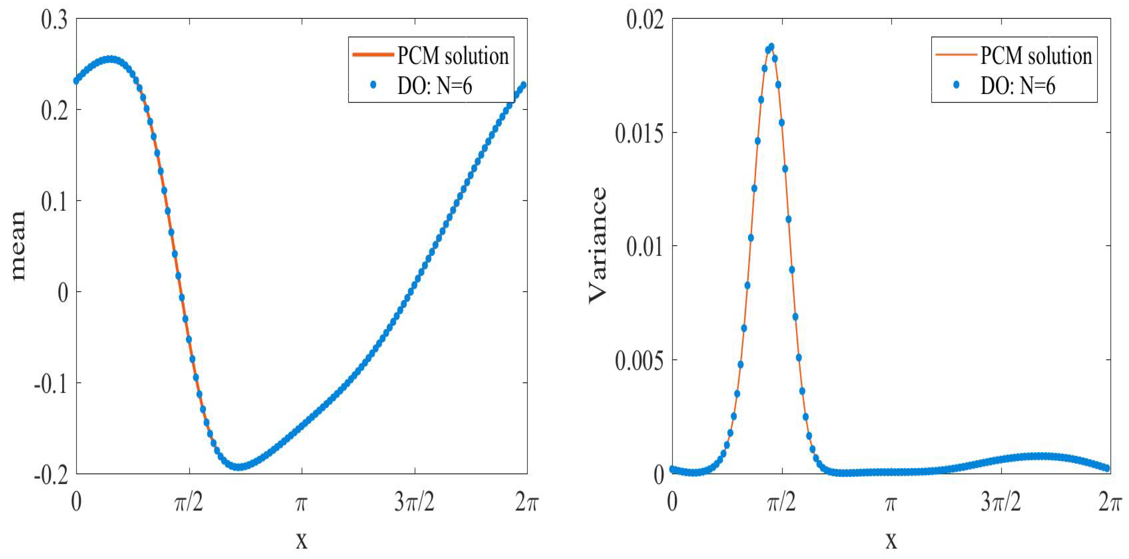
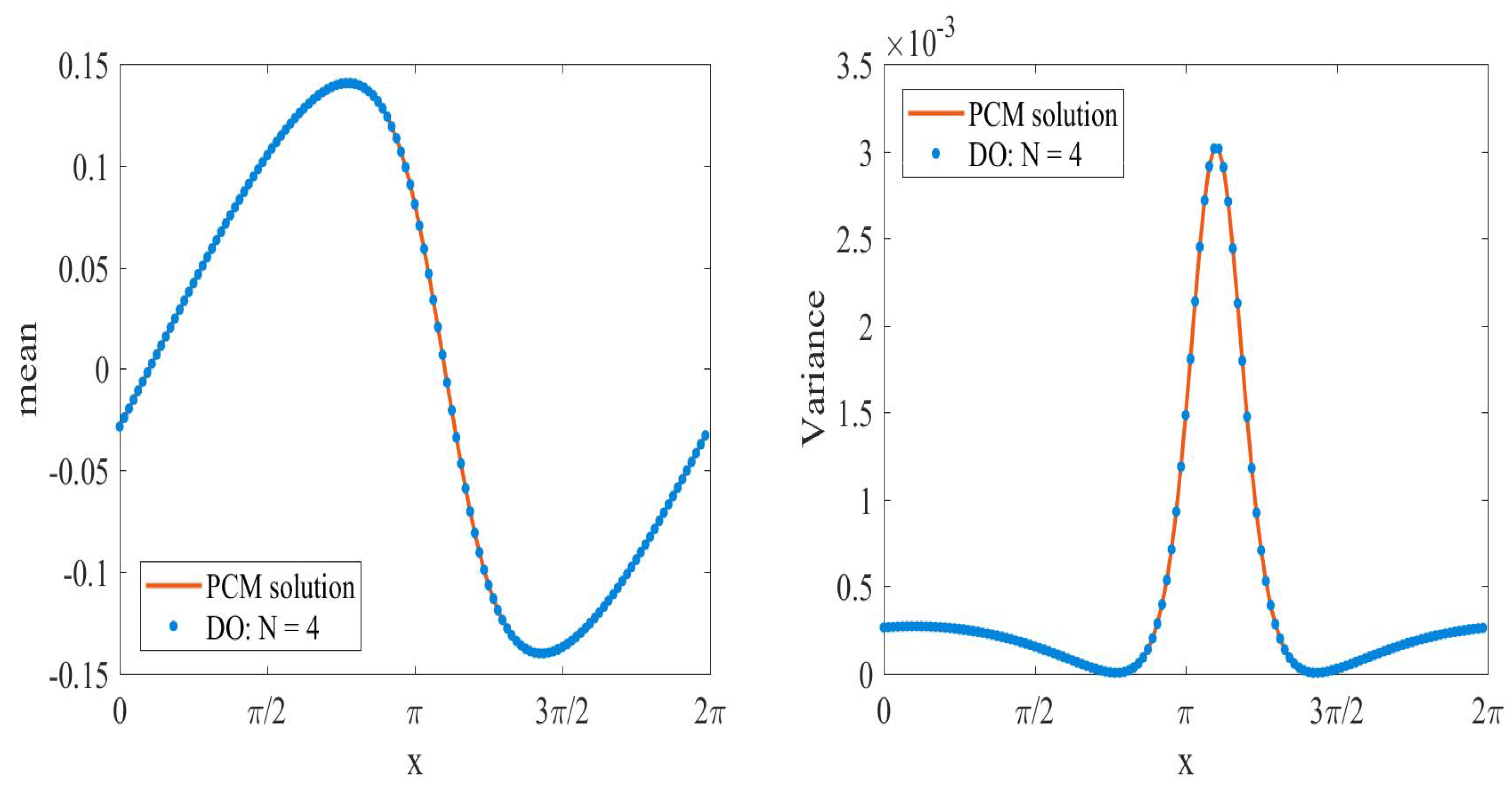
In Figure 1, the mean and variance are shown at t f = 5 and N = 6 . They agree well with the reference solution. The L 2 error for the mean and variance for different values of modes are shown in Figure 2. We present errors in mean and variance for three values of modes: N = 3 , N = 5 , and N = 7 . The solution at t s = 2 and N = 7 is the best among the three cases. To this end, it can be noticed that the accuracy of the solution is affected by lower modes.
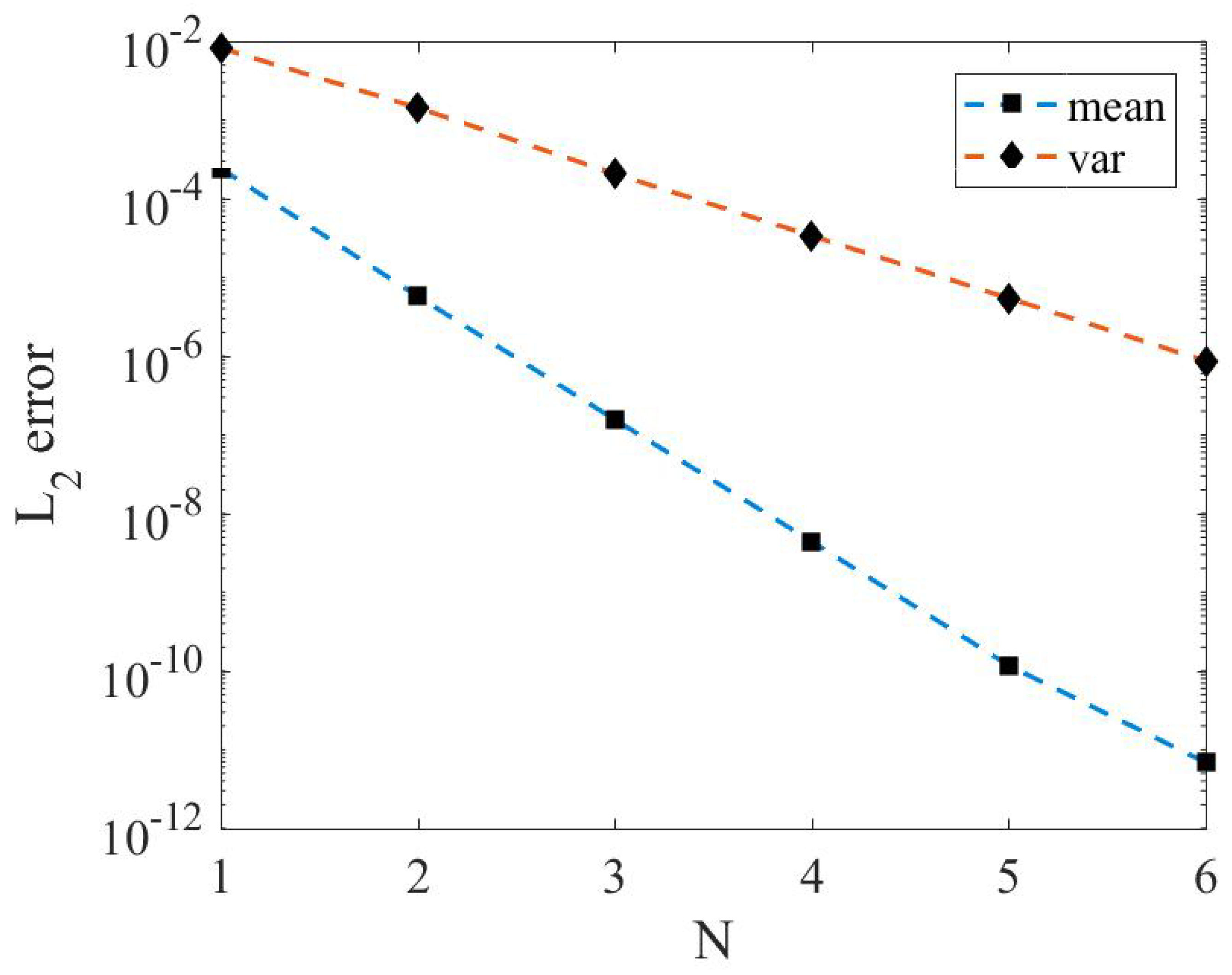
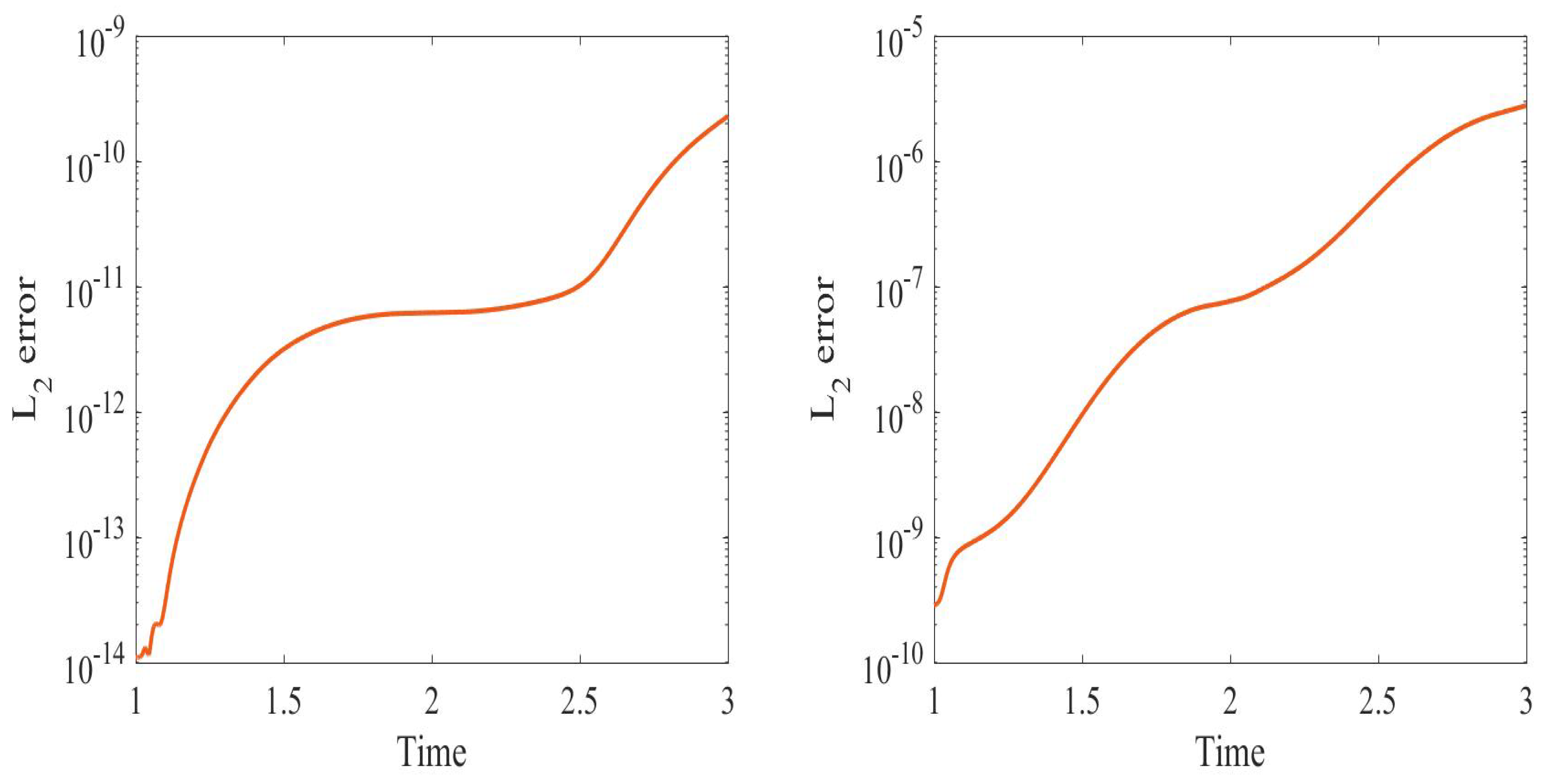
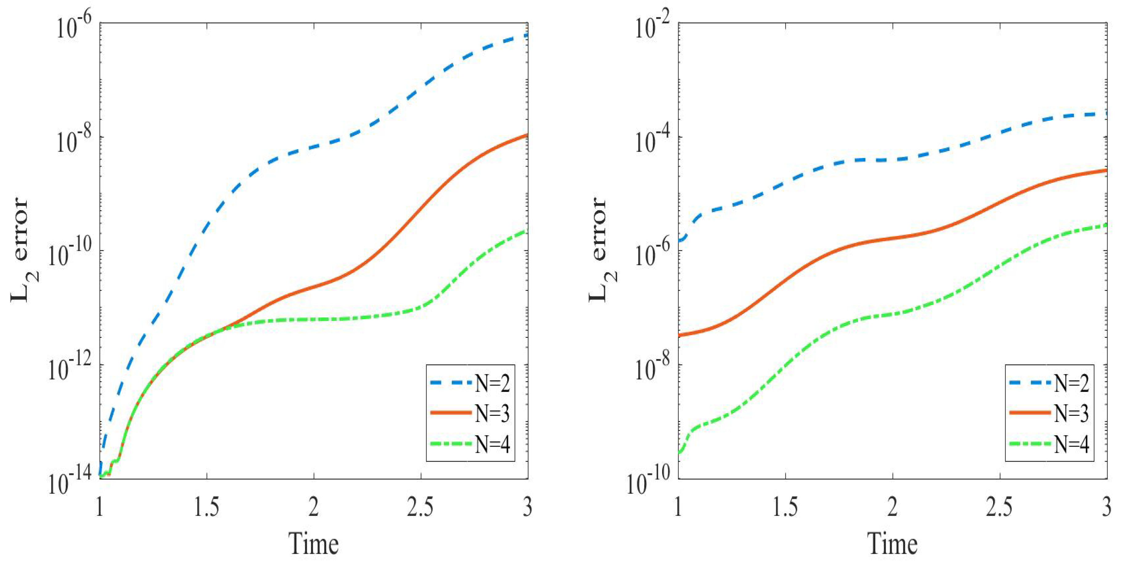
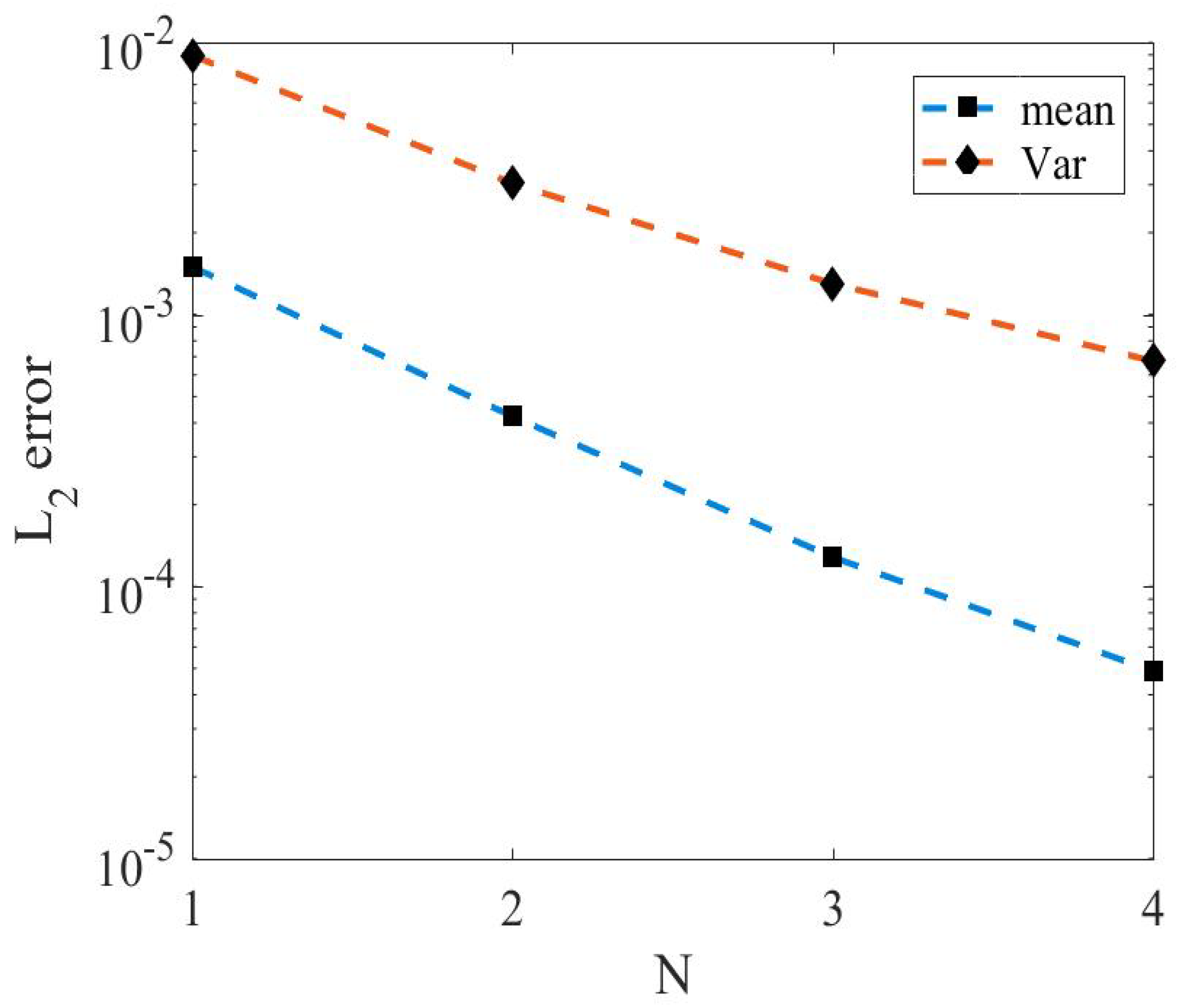
Figure 3 shows the high convergence rate detected with the number of modes. The L 2 error reduces as the number of modes increases. This demonstrates that the DO decomposition has a high convergence rate for this nonlinear case.
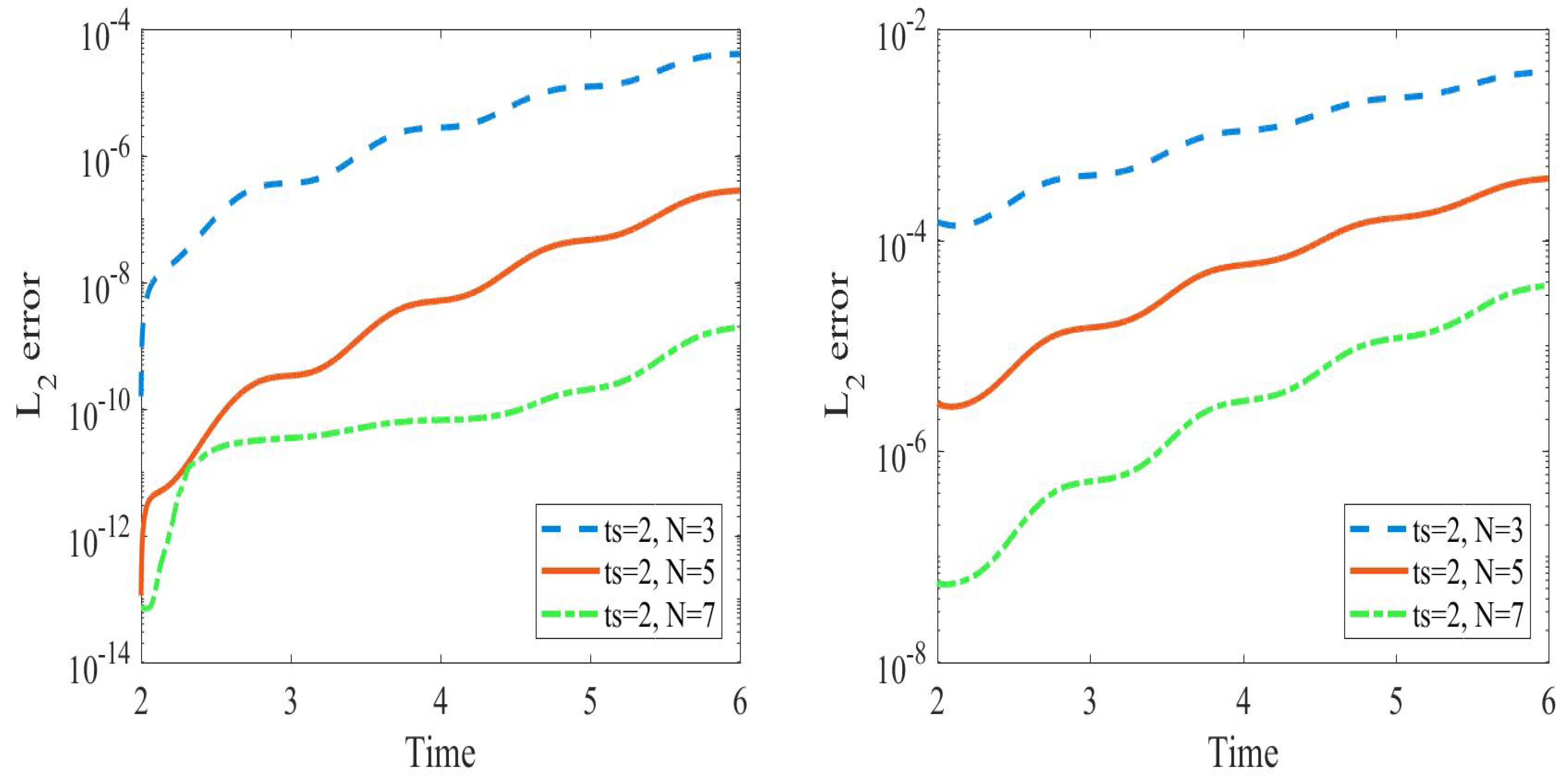
Figure 4 shows that the hybrid approach is affected by the switching time and number of modes. We observe that L 2 error for the mean and variance at t s = 1 and N = 6 is the best among other values. For t s = 2 and N = 6 
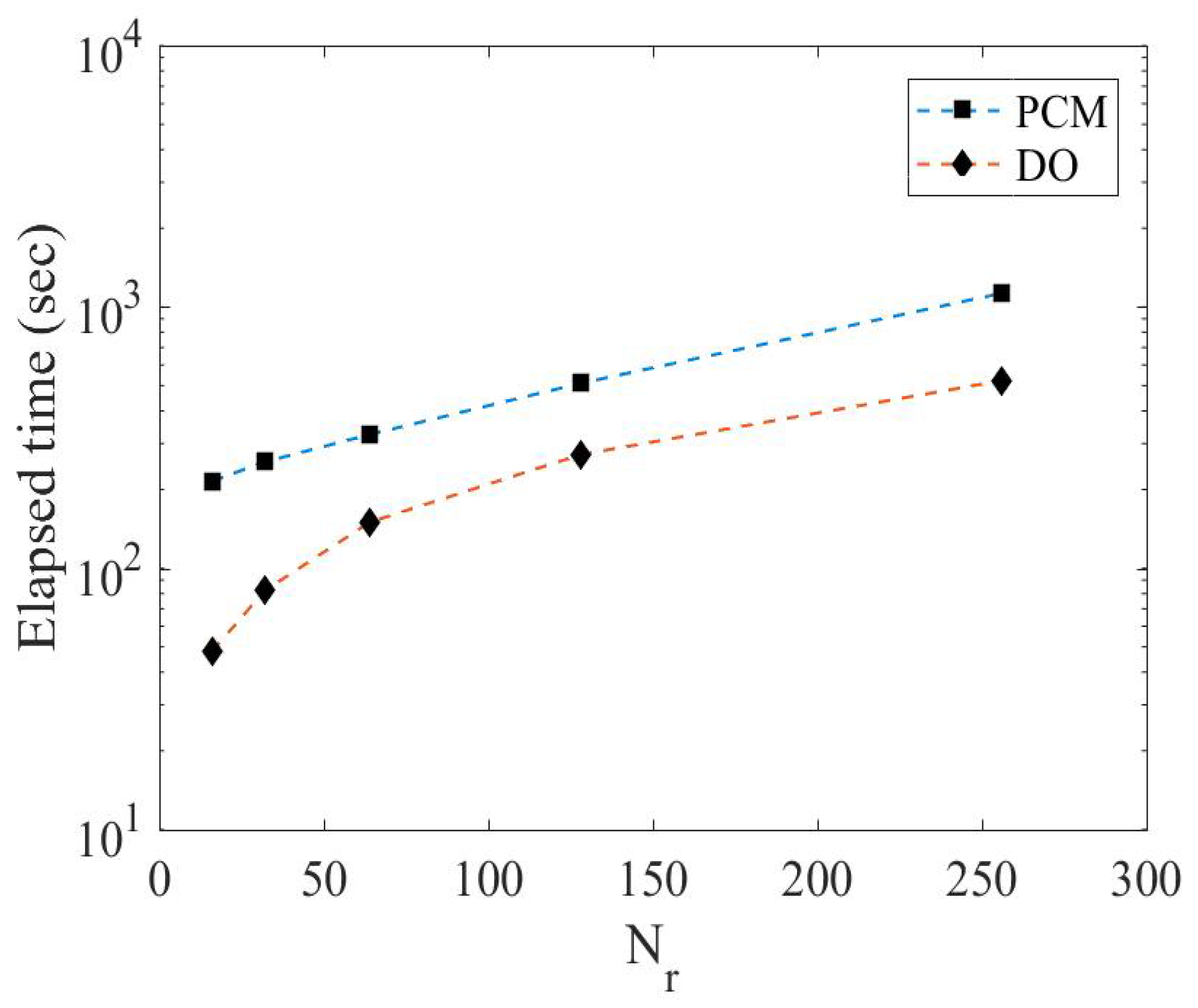
, the solution has the same accuracy but takes more computational time. The computational time is compared when using the DO and PCM for this test case using different spatial nodes Nr. The DO is more efficient, with less computational time than the PCM, as shown in Figure 5.
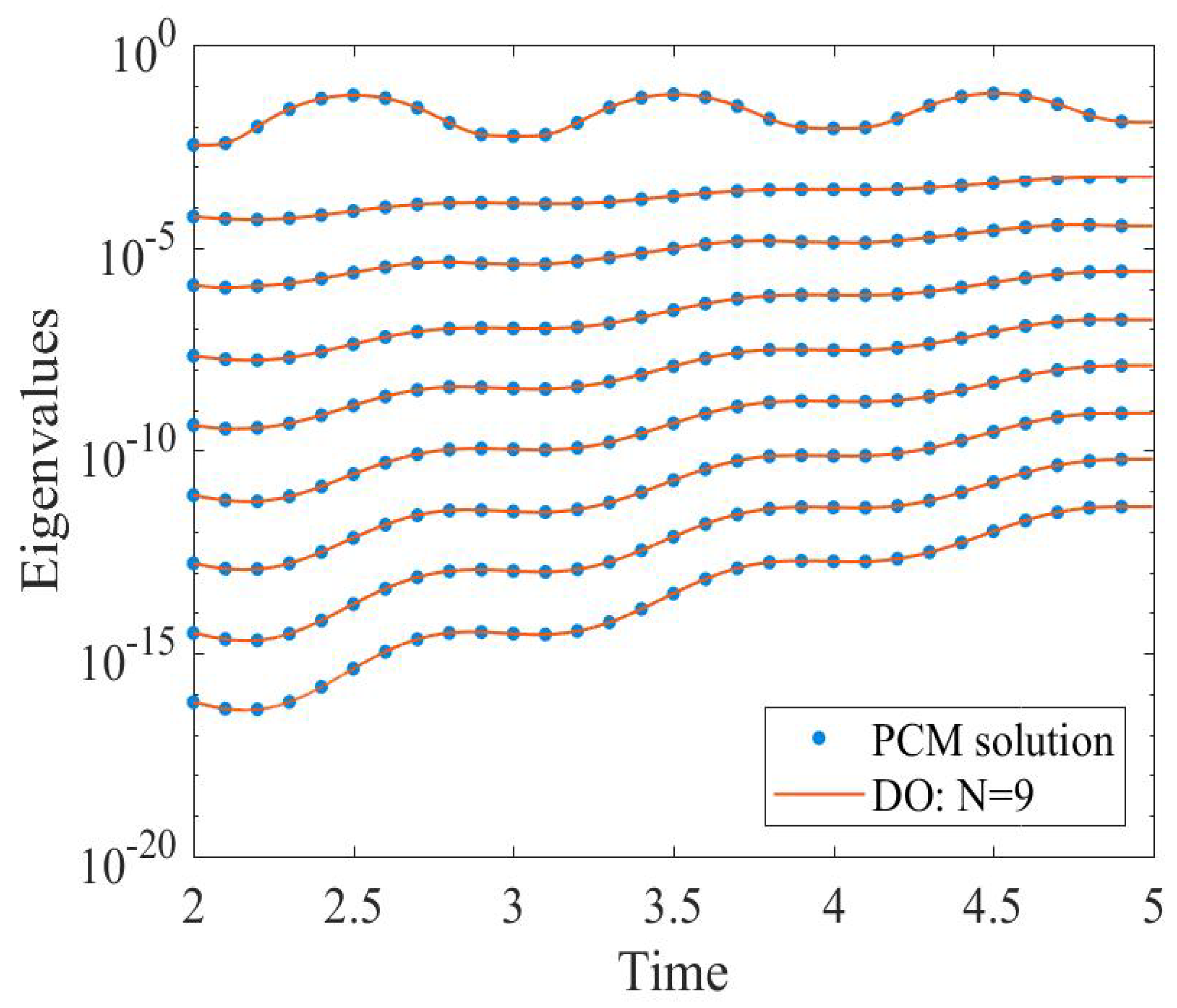
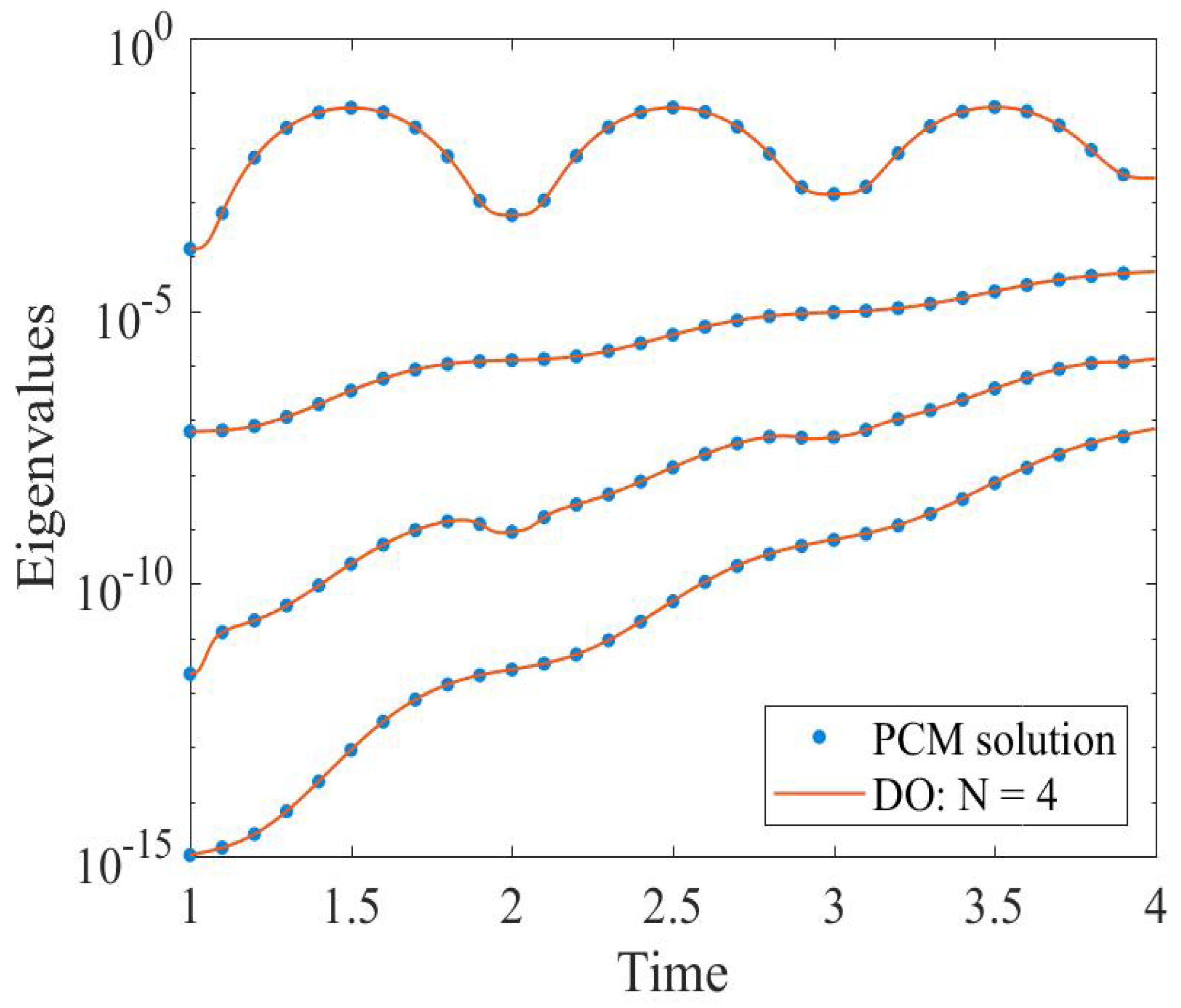
Figure 6 shows the eigenvalues variation as the solution evolves till t f = 5 . The computed eigenvalues are compared with the reference solution. A good agreement is noticed as shown in the figure. It is observed that the lower eigenvalues λ 8   and   λ 9 from the mode N = 9 have an order: 10 15   and   10 16 , respectively, making the covariance matrix extremely ill-conditioned; it becomes singular and hence sensitive to any perturbations.

3.2. Quasilinear Inviscid Burgers’ Equation

Consider the stochastic quasilinear inviscid Burgers’ equation with a random forcing in the form [36]:
u t + u   u x = 1 + ξ 2 sin 2 π t ; u x , 0 = g x ,  
where x 0 , 2 π   ,   t 0 ,   t f   ,   ξ   ~   U 1 , 1 with periodic boundary conditions and the initial condition is:
g x = 1 7   sin x .
Applying the DO decomposition to get the evolution operator L along with other forms:
  L u x , t ; ω = u t = u u x + 1 + ξ 2 sin 2 π t .
E L u = u ¯ u ¯ x C i j u i u j x + 0.5 sin 2 π t .
E L u   Y j = C i j u i   u ¯ x + C k j   u k x u ¯ + C i k j   u k x   + E   ξ 2 Y j sin 2 π t ,
where C i k j = E Y i Y k Y j . We shall use similar parameters as in the above example in Section 3.1.
Figure 7 demonstrates that errors in the mean and its variance are identical for both the DO and the PCM methods. We present mean and variance at time t f = 6 as shown in Figure 8. They have a good agreement compared with the reference solution. 
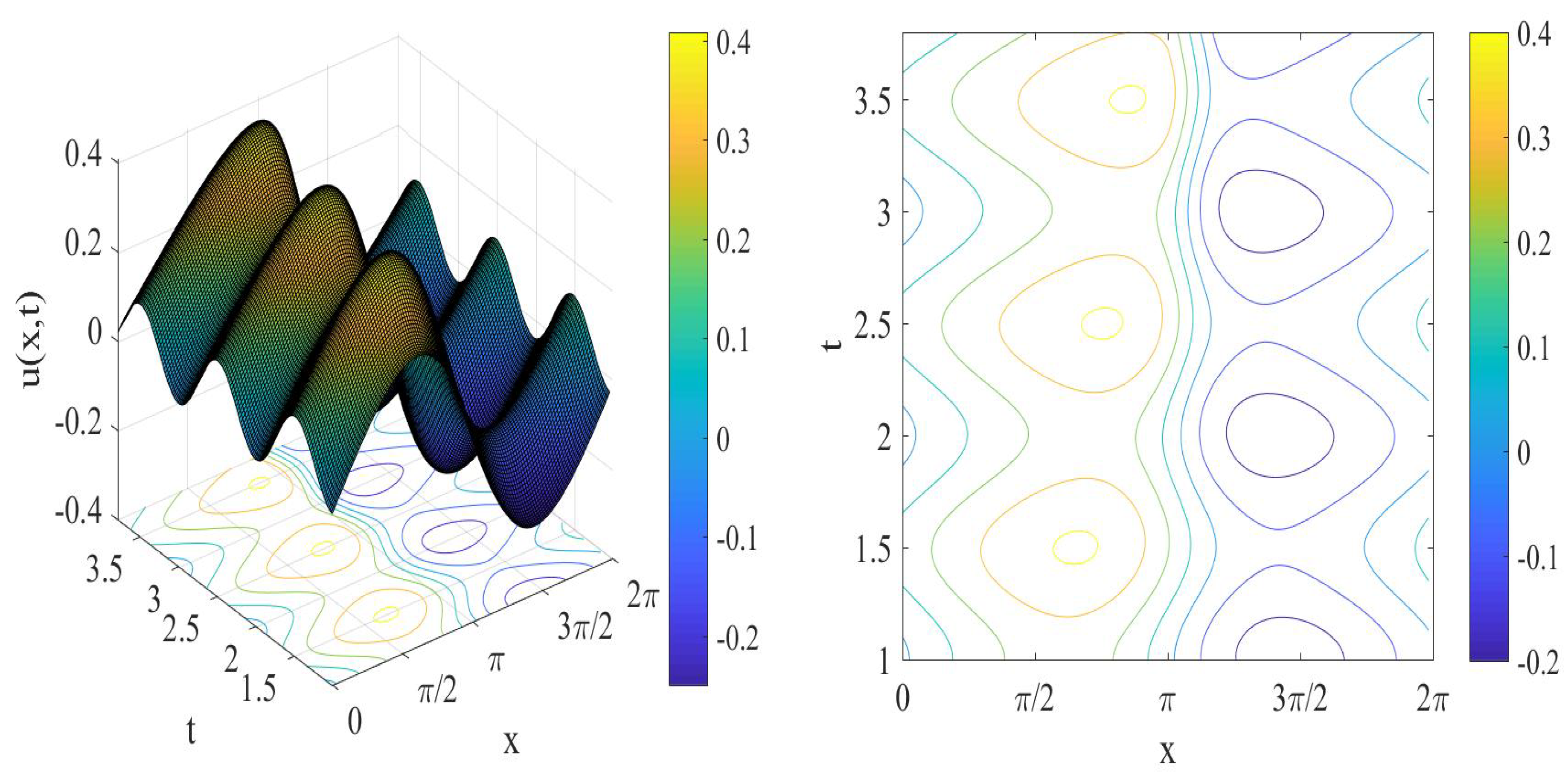
Figure 9 shows the performance of the mean solution u ¯ x , t using the DO method as the number of time iterations increases along with the contour lines. The solution is illustrated at t f = 6 at switching time t s = 1 and number of modes N = 4 with time increment t = 10 3 . We observe that the wave shape tends to be sharper with time. The L 2 error of the DO method for different modes number N are shown in Figure 10. We present the errors in the variance and mean for three modes N = 2 , N = 3   and   N = 4 with the same switching time t s = 1 . As shown, and as expected, the error due to mode N = 4 is less than errors due to other modes. Therefore, as the number of modes increases, the error is reduced. Figure 11 shows the high rate of error convergence with increasing the modes number. This implies that the DO representation is also an efficient choice for this nonlinear SPDE.
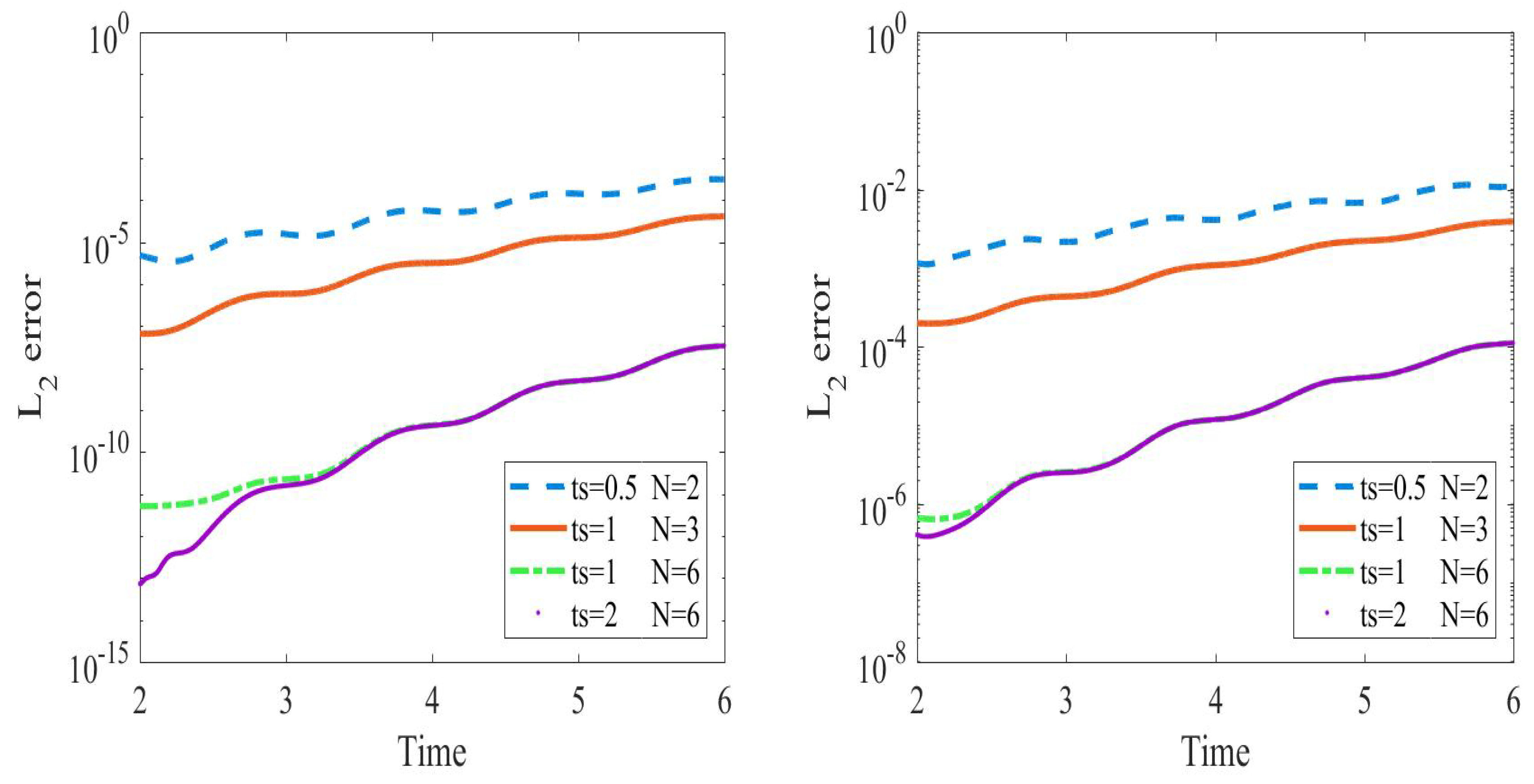
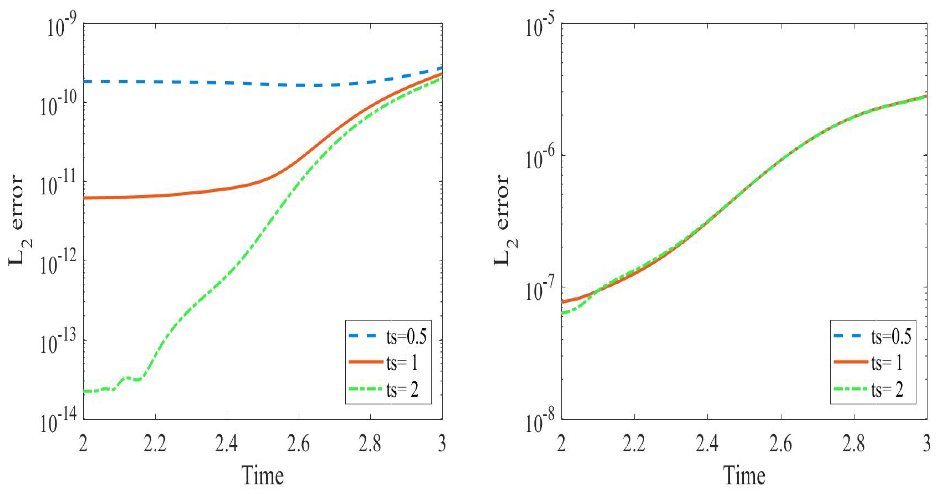
As it is shown in Figure 12, the L 2 error of the solution is computed for three switching times t s = 0.5 ,   t s = 1 and t s = 2 with the same number of modes N = 4 . We can observe that the error for the mean at t s = 2 is better than the errors due to other switching times. After that, the error becomes the same for the three modes. On the other hand, the error in variance is approximately the same for all switching times, so we can use t s = 1 as it has a smaller computational time.
Figure 13 shows the time growth of eigenvalues till t f = 6 . The computed eigenvalues are compared with those from the reference solution and a good agreement is achieved. It is observed that the smaller eigenvalues λ 3 and λ 4 have an order 10 15   and   10 12 , respectively. This means the covariance matrix is highly ill-conditioned and becomes singular as the modes number increases.

4. Shock Wave Occurrence

Consider the stochastic inviscid Burger’s equation with random forcing as follows:
u t + u   u x = 1 + ξ 2 sin 2 π t ; u x , 0 = g x ,  
where x 0 , 2 π   ,   t 0 ,   t f   ,   ξ   ~   U 1 , 1 with periodic boundary conditions and the initial condition to be taken as:
g x = 1 3   s i n x .
This model is the same model given in (32), but with different initial condition g x that allows for shock formation. We consider the solution up to a final time t f = 4 . The above described DO method in Section 2 is applied to the model Equation (37). The convective term u   u / x should be handled using any suitable technique such as first and/or second-order upwind scheme. This will prevent oscillatory behavior of the solution, especially near the shock wave. 
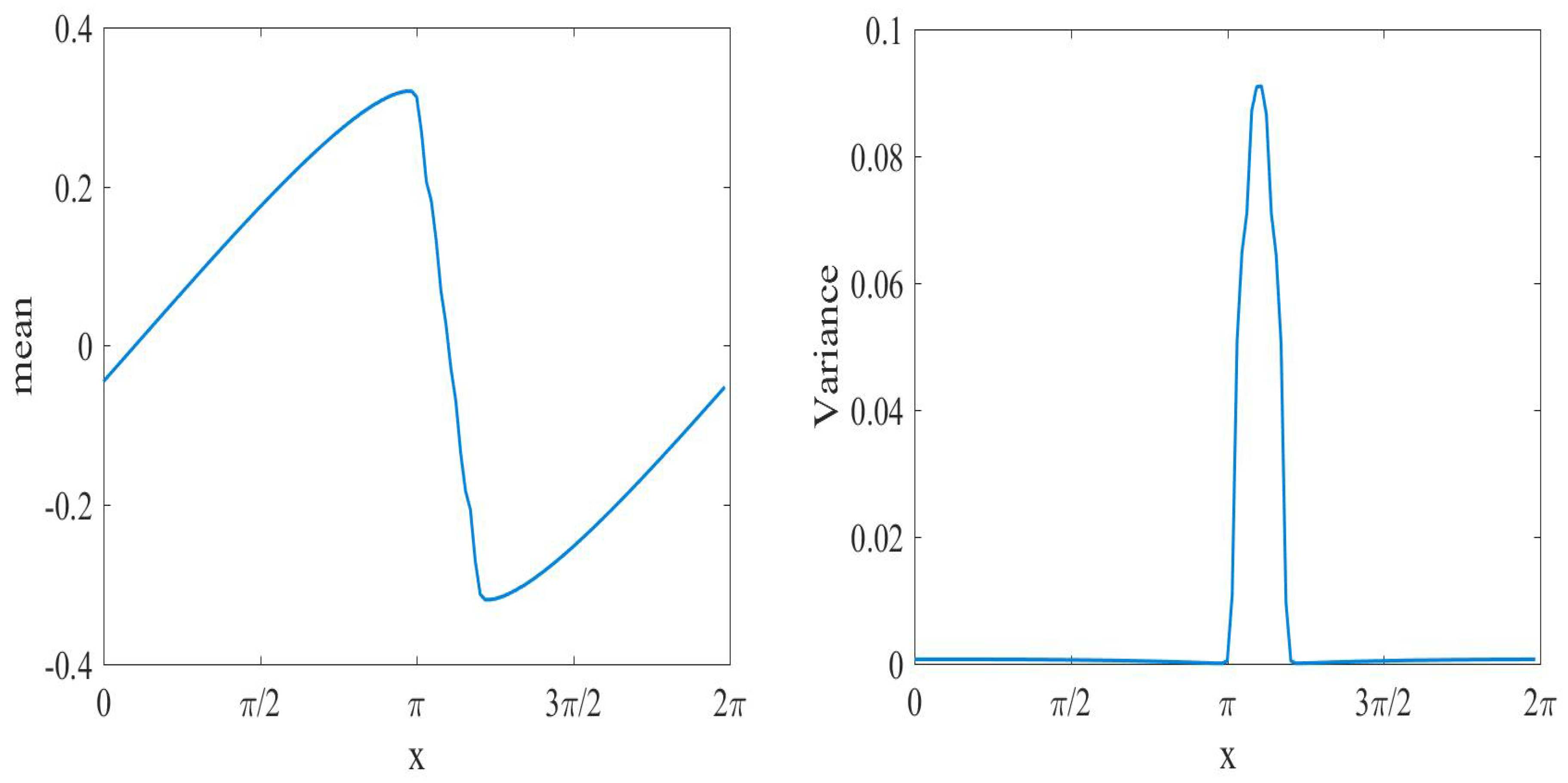
Figure 14 shows the solution mean and variance at the occurrence of the shock wave. The solution is illustrated at switching time t s = 1 , and the number of modes considered is N = 4 . As the waveform steepens, the edges form causing a shock wave. We can notice how variance become relatively large close to the shock wave. The maximum value of variance occurs exactly at the shock wave. The mean field u ¯ x , t 
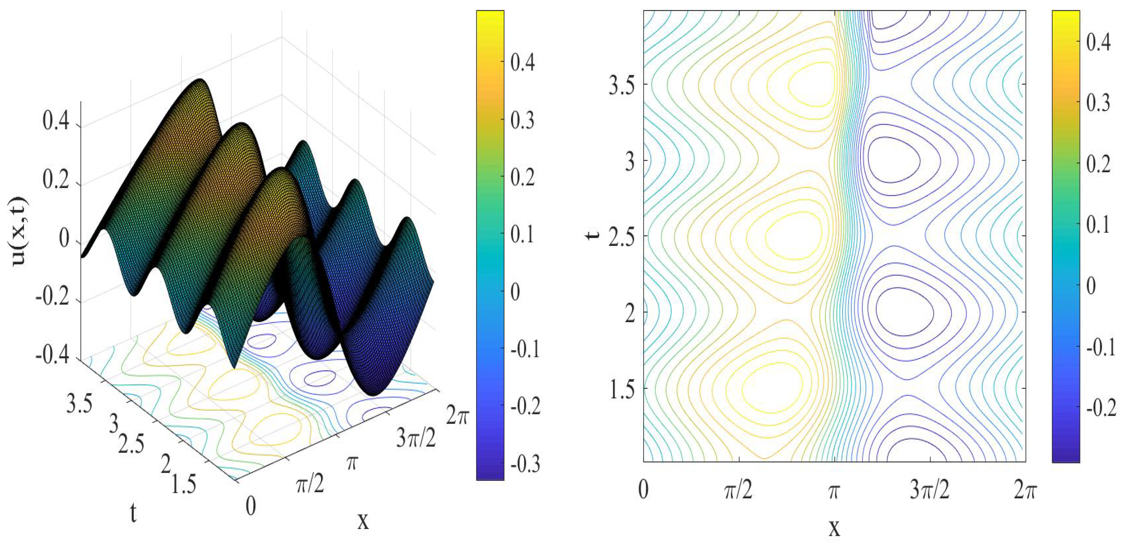
of the solution is shown in 
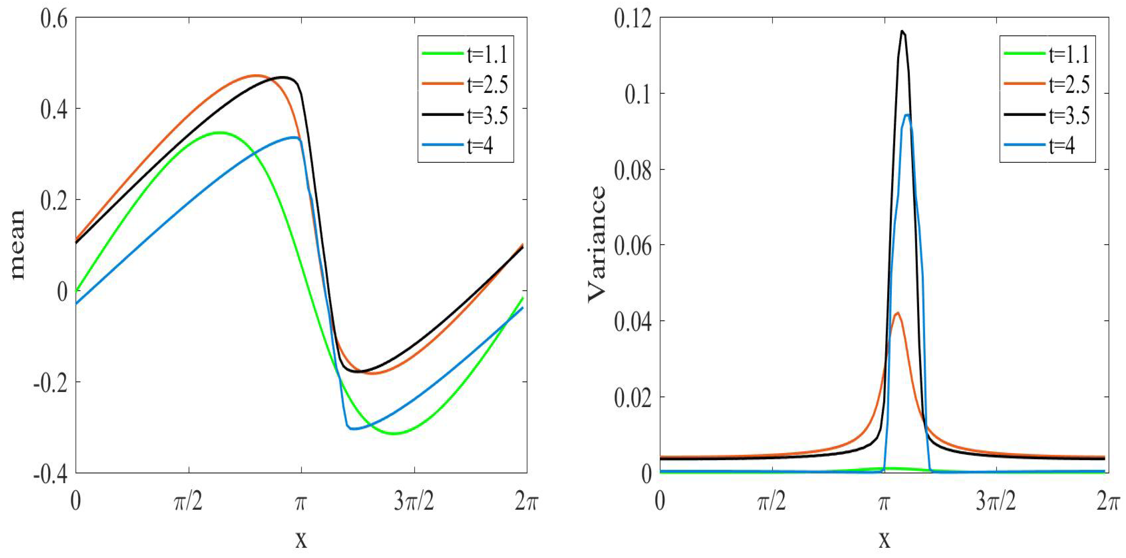
Figure 15. We present the mean field and the contour lines’ evolution up to the breaking time. The sinusoidal wave shape sharpens as the time evolves till the shock wave occurs. The mean and variance for the solution is sketched at different values of time as shown in Figure 16. Time values t = 1.1 ,   t = 2.5 ,   t = 3.5 , and t = 4 are considered in Figure 16. It can be observed that the sinusoidal wave shape is distorted. The distortion of the wave profile starts from the initial data, and the dispersion of the wave profile evolves with the time increase.

5. Conclusions

The Burgers’ model with stochastic terms is an important problem which appears in many applications such as the flow turbulence. Due to lack of analytical methods, numerical techniques are required to analyze such important models. The stochastic Burgers’ model is studied using DO and PCM methods in the current study. The DO method introduces a computational low-dimensional framework that enables to capture the relevant system dynamics for the stochastic Burgers’ model. The PCM is combined with the DO to avoid the singularity of the DO evolution in case of deterministic initial conditions. The approach is based on solving the model using the PCM up to a certain switching time at which the stochasticity occurs, and then switching to the DO method. The two strategies, DO and PCM-DO, are successfully applied to the stochastic Burgers’ model and are compared in terms of performance and accuracy with a reference solution. The stochastic viscous and inviscid Burgers’ models combined with random forces are considered with the two methods. We derived the quantities of the stochastic coefficients and spatial bases for these models. When analyzing the test models, the DO method shows a high level of agreement with the reference solution and has a convergence rate increase with the number of modes.
Overall, the DO method is as accurate as the PCM method, but with higher efficiency. This explains why the DO method could be a viable and gainful replacement for the PCM. We also analyzed the shock wave formation using the DO by considering the inviscid Burgers’ equation with suitable discretization of the convective tern to avoid oscillatory solution. The sinusoidal wave shape sharpens and distorts as the time evolves till the shock wave occurs. The mean solution shows the shock occurrence while the variance explains the magnification of oscillations close to shock formation. Further research should focus on more systematic studies to determine the suitable switching time from PCM to DO methods. Moreover, other applications are to be considered using the current presented techniques.

Author Contributions

Conceptualization, formal analysis, methodology, R.M. and M.E.-B.; investigation R.M. and A.N.; writing—original draft preparation, R.M. and M.E.-B.; Resources, Validation, A.N.; writing—review and editing, M.E.-B. and R.M. All authors have read and agreed to the published version of the manuscript.

Funding

This project was funded by the Deanship of Science Research (DSR) at King Abdulaziz University, Jeddah, Saudi Arabia, under grant no. D-331-611-1441. The authors, therefore, acknowledge with thanks to DSR for the technical and financial support.

Institutional Review Board Statement

Not applicable.

Informed Consent Statement

Not applicable.

Data Availability Statement

Not applicable.

Conflicts of Interest

The authors declare no conflict of interest.

References

  1. Grigoriu, M.; Soong, T.T. Random Vibration of Mechanical and Structural Systems; PTR Prentice Hall Inc.: Englewood Cliffs, NJ, USA, 1993. [Google Scholar]
  2. Lin, Y.; Cai, G. Probabilistic Structural Dynamics; McGraw-Hill Inc.: New York, NY, USA, 1995. [Google Scholar]
  3. Spanos, P.D.; Roberts, J.B. Random Vibration and Statistical Linearization; Courier Corporation: Chelmsford, MA, USA, 2003. [Google Scholar]
  4. Sobczyk, K. Stochastic Wave Propagation; Elsevier Publishing Company: Amsterdam, The Netherlands, 1985. [Google Scholar]
  5. Vazquez, L.; Konotop, V. Nonlinear Random Waves; World Scientific: Singapore, 1994. [Google Scholar]
  6. Solna, K.; Fouque, J.P.; Garnier, J.; Papanicolaou, G. Wave Propagation and Time Reversal in Randomly Layered Media; Springer Science & Business Media: Berlin, Germany, 2007; Volume 56. [Google Scholar]
  7. Giles, M.B. Multilevel monte carlo path simulation. Oper. Res. 2008, 56, 607–617. [Google Scholar] [CrossRef]
  8. Papadopoulos, C.E.; Yeung, H. Uncertainty estimation and Monte Carlo simulation method. Flow Meas. Instrum. 2001, 12, 291–298. [Google Scholar] [CrossRef]
  9. Barth, A.; Lang, A.; Schwab, C. Multilevel Monte Carlo method for parabolic stochastic partial differential equations. BIT Numer. Math. 2013, 53, 3–27. [Google Scholar] [CrossRef]
  10. Liu, J.S.; Liu, J.S. Monte Carlo Strategies in Scientific Computing; Springer: New York, NY, USA, 2001; Volume 10, p. 978. [Google Scholar]
  11. Gordon, N.; Doucet, A.; de Freitas, N. Sequential Monte-Carlo Methods in Practice; Springer: Berlin/Heidelberg, Germany, 2001. [Google Scholar]
  12. Hoteit, I.; Pham, D.T.; Triantafyllou, G.; Korres, G. A new approximate solution of the optimal nonlinear filter for data assimilation in meteorology and oceanograph. Mon. Weather Rev. 2008, 136, 317–334. [Google Scholar] [CrossRef]
  13. Lermusiaux, P.F. Uncertainty estimation and prediction for interdisciplinary ocean dynamics. J. Comput. Phys. 2006, 217, 176–199. [Google Scholar] [CrossRef]
  14. Lermusiaux, P.F.; Chiu, C.S.; Gawarkiewicz, G.G.; Abbot, P.; Robinson, A.R.; Miller, R.N.; Lekien, F. Quantifying Uncertainties in Ocean Predictions; Harvard Univ Cambridge: Cambridge, MA, USA, 2006; Volume 19, pp. 92–105. [Google Scholar]
  15. Nagy, S.A.; El-Beltagy, M.A.; Wafa, M. Multilevel Monte Carlo by using the Halton sequence. Monte Carlo Methods Appl. 2020, 26, 193–203. [Google Scholar] [CrossRef]
  16. Holmes, P.; Lumley, J.; Berkooz, G. Turbulence, Coherent Structures, Dynamical Systems and Symmetry; Cambridge University Press: Cambridge, UK, 1996. [Google Scholar]
  17. Ghanem, R.; Spanos, P. Stochastic Finite Elements: A Spectral Approach; Springer: Berlin/Heidelberg, Germany, 1991. [Google Scholar]
  18. Das, S.; Ghanem, R.; Finette, S. Polynomial chaos representation of spatiotemporal random fields from experimental measurements. J. Comput. Phys. 2009, 228, 8726–8751. [Google Scholar] [CrossRef]
  19. Xiu, D.; Karniadakis, G.E. The Wiener—Askey polynomial chaos for stochastic differential equations. SIAM J. Sci. Comput. 2002, 24, 619–6442. [Google Scholar] [CrossRef]
  20. Xiu, D.; Em Karniadakis, G. Modeling uncertainty in flow simulations via generalized polynomial chaos. J. Comput. Phys. 2003, 187, 137–167. [Google Scholar] [CrossRef]
  21. Jardak, M.; Su, C.H.; Karniadakis, G.E. Spectral polynomial chaos solutions of the stochastic advection equation. J. Sci. Comput. 2002, 17, 319–338. [Google Scholar] [CrossRef]
  22. Xiu, D.; Hesthaven, J.S. High-order collocation methods for differential equations with random inputs. SIAM J. Sci. Comput. 2005, 27, 1118–1139. [Google Scholar] [CrossRef]
  23. Karniadakis, G.E.; Foo, J. Multi-element probabilistic collocation method in high dimensions. J. Comput. Phys. 2010, 229, 1536–1557. [Google Scholar]
  24. El-Beltagy, M. A practical comparison between the spectral techniques in solving the SDEs. Eng. Comput. 2019, 36, 2369–2402. [Google Scholar] [CrossRef]
  25. El-Beltagy, M.; Etman, A.; Maged, S. Development of a fractional Wiener-Hermite expansion for analyzing the fractional stochastic models. Chaos Solitons Fractals 2022, 156, 111847. [Google Scholar] [CrossRef]
  26. Sapsis, T.P.; Lermusiaux, P.F. Dynamically orthogonal field equations for continuous stochastic dynamical systems. Phys. D Nonlinear Phenom. 2009, 238, 2347–2360. [Google Scholar] [CrossRef]
  27. Choi, M.; Sapsis, T.P.; Karniadakis, G.E. On the equivalence of dynamically orthogonal and bi-orthogonal methods: Theory and numerical simulations. J. Comput. Phys. 2014, 270, 1–20. [Google Scholar] [CrossRef]
  28. Karniadakis, G.E.; Choi, M.; Sapsis, T.P. A convergence study for SPDEs using combined polynomial chaos and dynamically-orthogonal schemes. J. Comput. Phys. 2013, 245, 281–301. [Google Scholar]
  29. El-Beltagy, M.; Wafa, M.; Galal, O. Upwind Finite-Volume Solution of Stochastic Burgers’ Equation. Appl. Math. 2012, 2, 1818–1825. [Google Scholar] [CrossRef]
  30. Rozanov, Y. Random Fields and Stochastic Partial Differential Equations; Kluwer Academic Press: Norwell, MA, USA, 1996. [Google Scholar]
  31. Naylor, A.; Sell, G. Linear Operator Theory in Engineering and Science; Springer: Berlin/Heidelberg, Germany, 1982. [Google Scholar]
  32. Babaee, H.; Choi, M.; Sapsis, T.P.; Karniadakis, G.E. A robust bi-orthogonal/dynamically-orthogonal method using the covariance pseudo-inverse with application to stochastic flow problem. J. Comput. Phys. 2017, 344, 303–319. [Google Scholar] [CrossRef]
  33. Foo, J.; Wan, X.; Karniadakis, G.E. The multi-element probabilistic collocation method (ME-PCM): Error analysis and applications. J. Comput. Phys. 2008, 227, 9572–9595. [Google Scholar] [CrossRef]
  34. Patil, P.; Babaee, H. Real-time reduced-order modeling of stochastic partial differential equations via time-dependent subspaces. J. Comput. Phys. 2020, 415, 109511. [Google Scholar] [CrossRef]
  35. Babaee, H. An observation-driven time-dependent basis for a reduced description of transient stochastic systems. Proc. R. Soc. A 2019, 475, 20190506. [Google Scholar] [CrossRef] [PubMed] [Green Version]
  36. Geiser, J.; Bartecki, K. Iterative and Non-Iterative Splitting Approach of the Stochastic Inviscid Burgers’ Equation; AIP Publishing LLC: Annapolis, MD, USA, 2020. [Google Scholar]
Figure 1. The mean (left) and variance (right) at t f = 5 , with the switching time t s = 1 and the number of modes N = 6 . The reference solution is RK4 from the PCM method.
Axioms 12 00152 g001
Figure 2. Mean L 2 error (left) and variance L 2 error (right) at t f = 6 . The switching time t s = 2 with different modes N = 3 ,   N = 5   and N = 7   is proposed.
Axioms 12 00152 g002
Figure 3. Mean (below) and variance (above) L 2 errors at t f = 3 . The switching time t s = 1 with different numbers of modes N.
Axioms 12 00152 g003
Figure 4. Burgers’ equation L 2 errors for mean solution (left) and its variance (right) at t f = 6 . The DO method is penetrating to the switching time t s and number of modes N .
Axioms 12 00152 g004
Figure 5. Burgers’ equation: The computational time against number of points (in spatial dimension) for both the PCM and DO methods.
Axioms 12 00152 g005
Figure 6. Burgers’ equation: The development in eigenvalues up to final time t f = 5 , switching time t s = 2 and the number of modes N = 9 .
Axioms 12 00152 g006
Figure 7. Mean L 2 error (left) and variance L 2 error (right) for the inviscid Burgers’ equation at t f = 3 and switching time t s = 1 with the number of modes N = 4 .
Axioms 12 00152 g007
Figure 8. The mean of the solution (left) and its variance (right) for the inviscid Burgers’ equation at t f = 4 , switching time t s = 1 with modes N = 4 . The reference solution is the PCM solution.
Axioms 12 00152 g008
Figure 9. The mean field u ¯ x , t (left) and contour lines (right) for the inviscid Burgers’ equation using the DO method at t f = 4 , switching at t s = 1 with number of modes N = 4 .
Axioms 12 00152 g009
Figure 10. Mean L 2 error (left) and variance error (right) for the inviscid Burgers’ equation at t f = 3 , switching at t s = 1 with different modes: N = 2 ,   N = 3   and N = 4 .
Axioms 12 00152 g010
Figure 11. Mean and variance L 2 errors for the inviscid Burgers’ equation at t f = 6 , switching at t s = 1 with different numbers of modes.
Axioms 12 00152 g011
Figure 12. Mean L 2 error (left) and variance L 2 error (right) for the inviscid Burgers’ equation of t f = 3 .
Axioms 12 00152 g012
Figure 13. Inviscid Burgers’ equation: Time evolution in eigenvalues with the final time t f = 4 , switching time t s = 1 and the number of modes N = 4 .
Axioms 12 00152 g013
Figure 14. The mean solution (left) and its variance (right) for the inviscid Burgers’ equation switching at t s = 1 with modes number N = 4 .
Axioms 12 00152 g014
Figure 15. The mean solution field u ¯ x , t (left) and its contour lines (right) for the inviscid Burgers’ equation using the DO method.
Axioms 12 00152 g015
Figure 16. The mean solution (left) and its variance (right) for the inviscid Burgers’ model at difference times up to shock occurrence.
Axioms 12 00152 g016
Disclaimer/Publisher’s Note: The statements, opinions and data contained in all publications are solely those of the individual author(s) and contributor(s) and not of MDPI and/or the editor(s). MDPI and/or the editor(s) disclaim responsibility for any injury to people or property resulting from any ideas, methods, instructions or products referred to in the content.

