
An Efficient Method for Solving Two-Dimensional Partial Differential Equations with the Deep Operator Network
Abstract
:1. Introduction
- To obtain enough two-dimensional PDE data for training, we design a method to construct binary functions in the classical function space and obtain the corresponding PDE solutions through the difference method to form point-value data sets. To prove the DeepONet output is closer to the actual value, we analyze the constructed function theoretically that can be applied for model training.
- To solve the challenge of the form of the input data, we rely on DeepONet to design a new data dimensionality reduction algorithm. This method flattens the matrix data representing the function into vectors for inputting the branch network and randomly selects the location and time information as the trunk network input.
- The proposed strategy is performed on the two-dimensional Poisson equation and the heat conduction equation experiments. Compared with other methods, we verify that it is accurate and efficient in predicting two-dimensional PDEs.
2. Methodology
2.1. Deep Operator Network Architecture
| Algorithm 1 Function dimensionality reduction |
| input function output discrete points vector F represents the function
|
2.2. The Data Set and Training Scheme
| Algorithm 2 Training strategy one |
| input input function F, independent variable output triples
|
| Algorithm 3 Training strategy two |
| input input function F, independent variable output triples
|
3. Problem Formulation
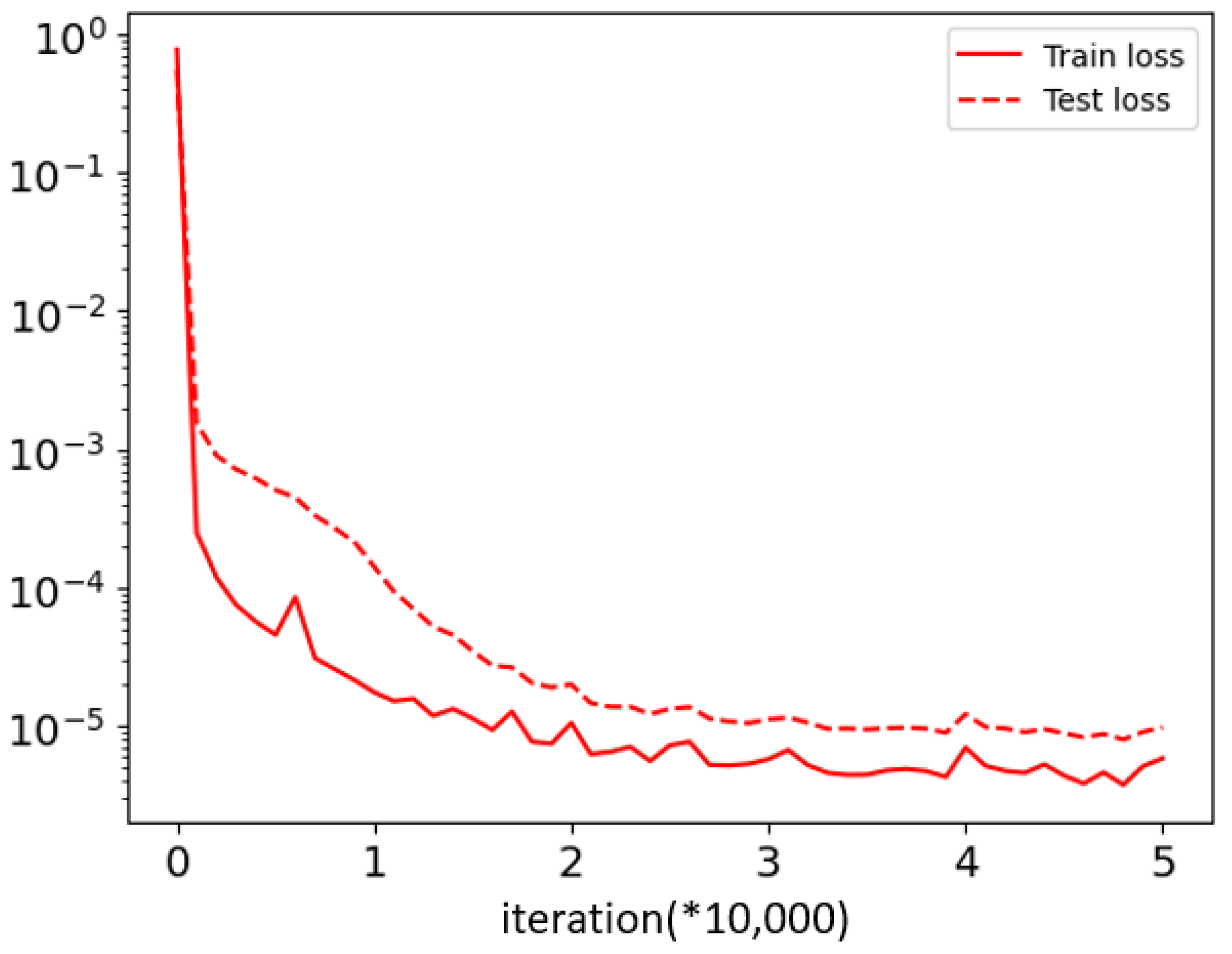
4. Experimental Results
4.1. Experimental Setup
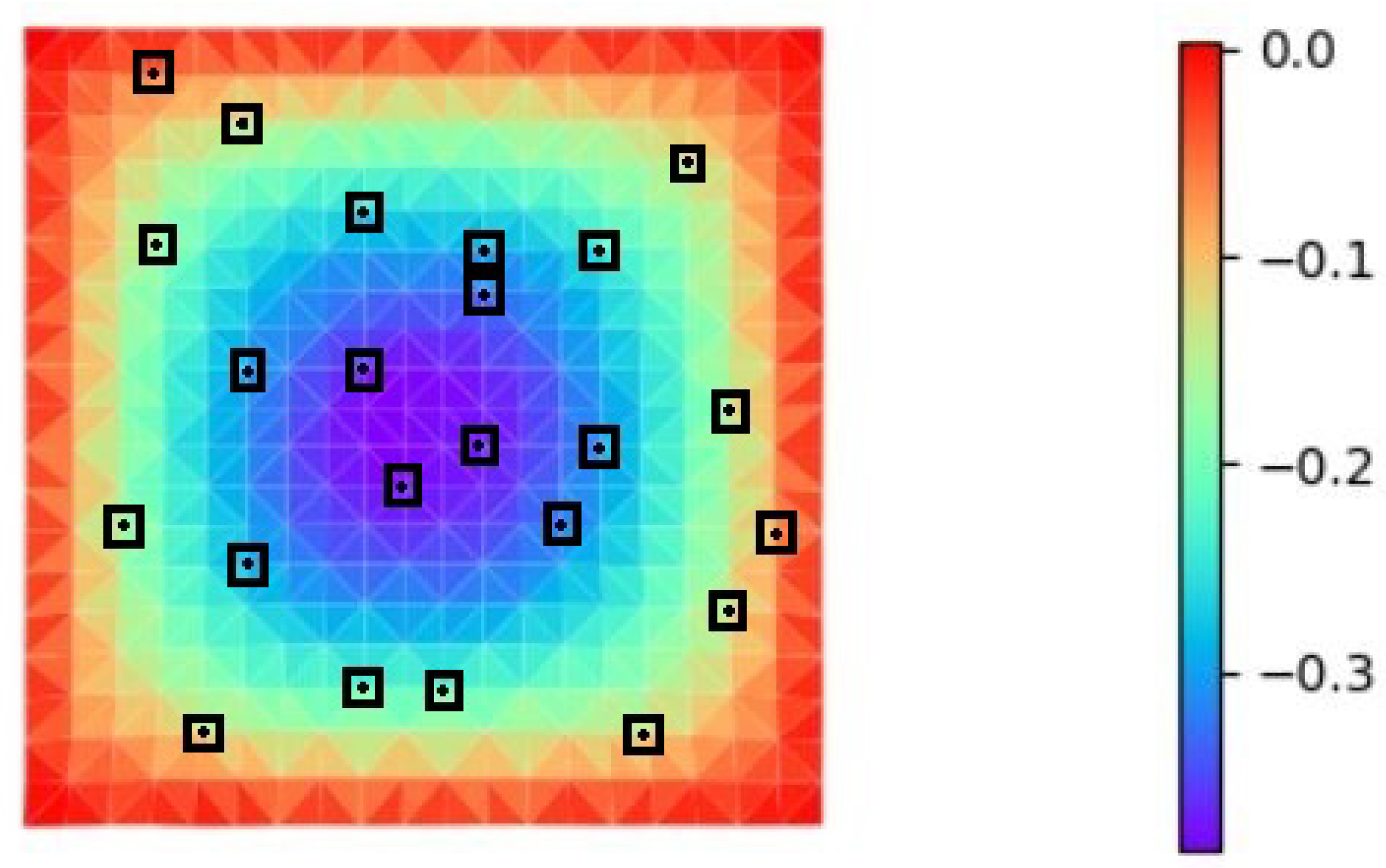
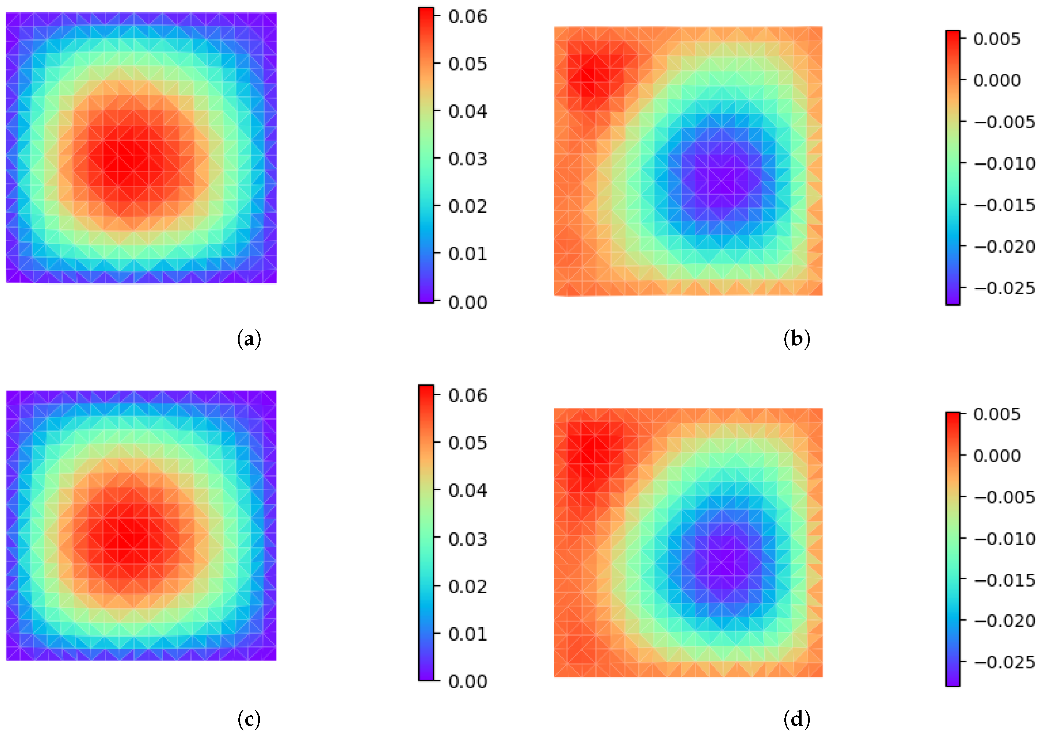
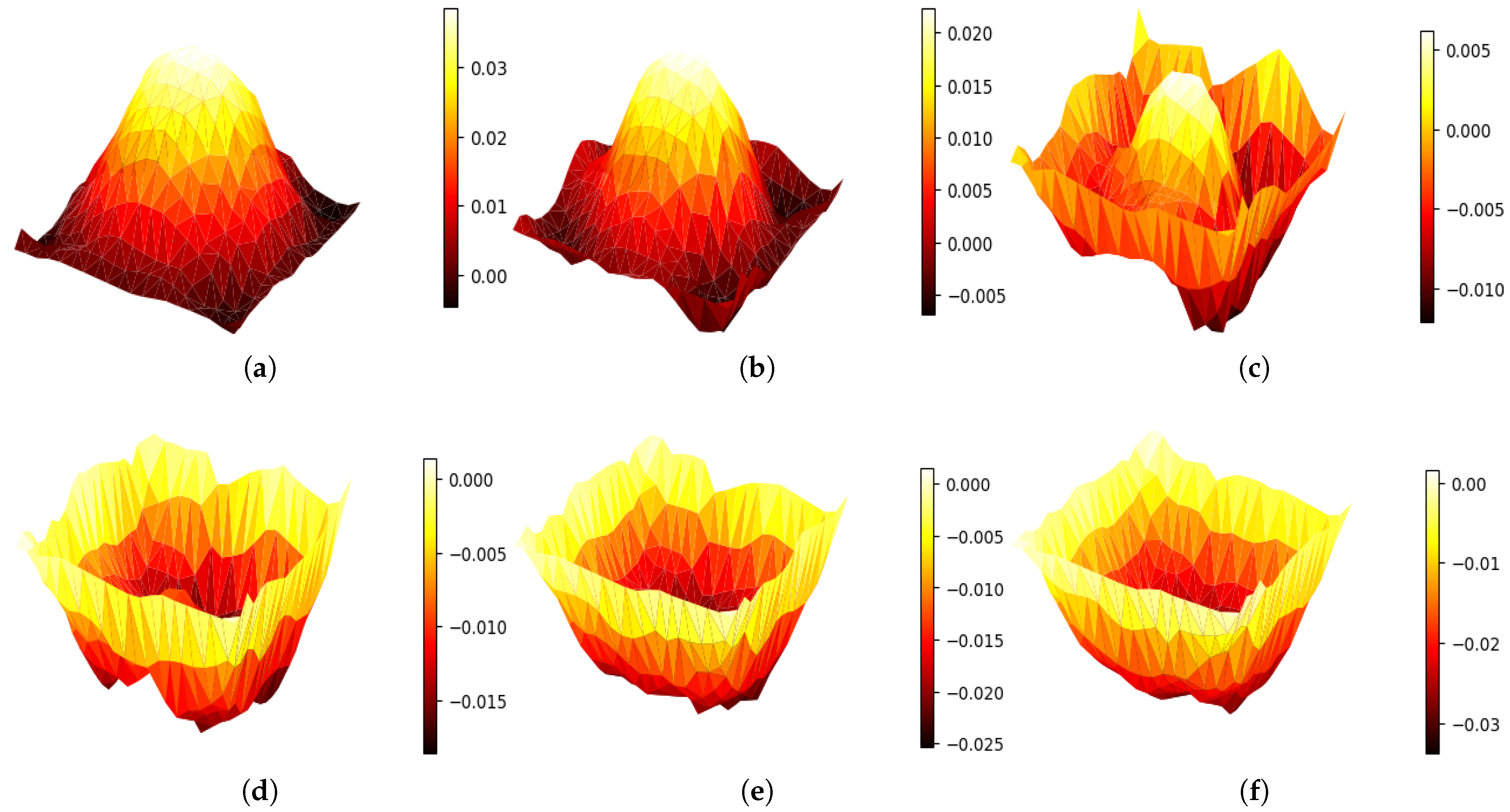
4.2. Poisson Equation
4.3. Heat Conduction Equation
4.3.1. Number of Input Functions
4.3.2. Number of Training Data Points
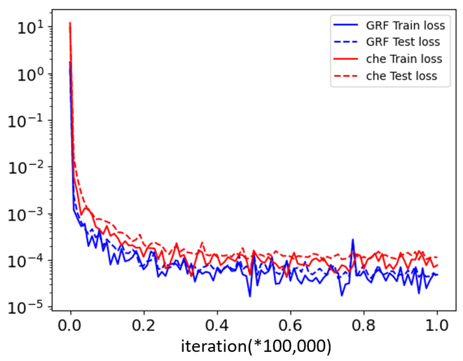
4.3.3. Different Function Spaces
4.3.4. Discrete Points
4.3.5. Different Training Method
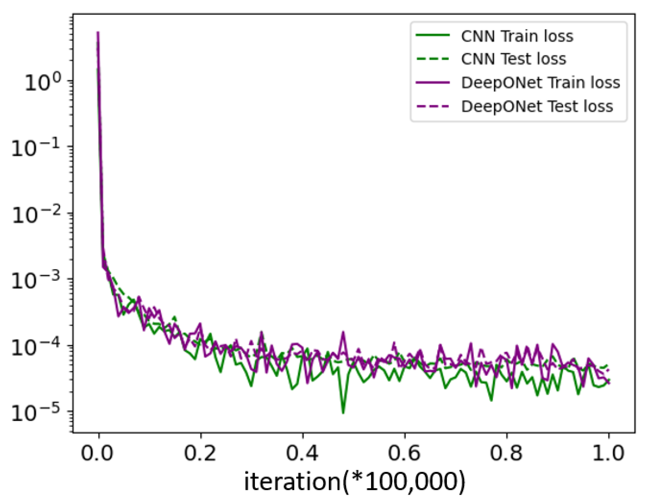
4.3.6. Different Models
5. Conclusions
Author Contributions
Funding
Data Availability Statement
Acknowledgments
Conflicts of Interest
References
- Øksendal, B. Stochastic partial differential equations and applications to hydrodynamics. In Stochastic Analysis and Applications in Physics; Springer: Berlin/Heidelberg, Germany, 1994; pp. 283–305. [Google Scholar]
- Constantin, P. Analysis of Hydrodynamic Models; SIAM: Philadelphia, PA, USA, 2017. [Google Scholar]
- Lenhart, S.; Xiong, J.; Yong, J. Optimal controls for stochastic partial differential equations with an application in population modeling. SIAM J. Control Optim. 2016, 54, 495–535. [Google Scholar] [CrossRef]
- Thonhofer, E.; Palau, T.; Kuhn, A.; Jakubek, S.; Kozek, M. Macroscopic traffic model for large scale urban traffic network design. Simul. Model. Pract. Theory 2018, 80, 32–49. [Google Scholar] [CrossRef]
- Boureghda, A. A modified variable time step method for solving ice melting problem. J. Differ. Equations Appl. 2012, 18, 1443–1455. [Google Scholar] [CrossRef]
- Rao, S.S. The Finite Element Method in Engineering; Butterworth-heinemann: Oxford, UK, 2017. [Google Scholar]
- Shen, J.; Tang, T.; Wang, L.L. Spectral Methods: Algorithms, Analysis and Applications; Springer Science & Business Media: Berlin/Heidelberg, Germany, 2011; Volume 41. [Google Scholar]
- Aliabadi, F.M. Boundary element methods. In Encyclopedia of Continuum Mechanics; Springer: Berlin/Heidelberg, Germany, 2020; pp. 182–193. [Google Scholar]
- Moukalled, F.; Mangani, L.; Darwish, M.; Moukalled, F.; Mangani, L.; Darwish, M. The Finite Volume Method; Springer: Berlin/Heidelberg, Germany, 2016. [Google Scholar]
- Rubinstein, R.Y.; Kroese, D.P. Simulation and the Monte Carlo Method; John Wiley & Sons: Hoboken, NJ, USA, 2016. [Google Scholar]
- Sharma, D.; Goyal, K.; Singla, R.K. A curvelet method for numerical solution of partial differential equations. Appl. Numer. Math. 2020, 148, 28–44. [Google Scholar] [CrossRef]
- Liu, Z.; Xu, Q. A Multiscale RBF Collocation Method for the Numerical Solution of Partial Differential Equations. Mathematics 2019, 7, 964. [Google Scholar] [CrossRef]
- Aziz, I.; Amin, R. Numerical solution of a class of delay differential and delay partial differential equations via Haar wavelet. Appl. Math. Model. 2016, 40, 10286–10299. [Google Scholar] [CrossRef]
- Fahim, A.; Araghi, M.A.F.; Rashidinia, J.; Jalalvand, M. Numerical solution of Volterra partial integro-differential equations based on sinc-collocation method. Adv. Differ. Equations 2017, 2017, 362. [Google Scholar] [CrossRef]
- Sirignano, J.; Spiliopoulos, K. DGM: A deep learning algorithm for solving partial differential equations. J. Comput. Phys. 2018, 375, 1339–1364. [Google Scholar] [CrossRef]
- Raissi, M.; Perdikaris, P.; Karniadakis, G.E. Physics-informed neural networks: A deep learning framework for solving forward and inverse problems involving nonlinear partial differential equations. J. Comput. Phys. 2019, 378, 686–707. [Google Scholar] [CrossRef]
- Fang, Z. A high-efficient hybrid physics-informed neural networks based on convolutional neural network. IEEE Trans. Neural Netw. Learn. Syst. 2021, 33, 5514–5526. [Google Scholar] [CrossRef] [PubMed]
- Wang, K.; Chen, Y.; Mehana, M.; Lubbers, N.; Bennett, K.C.; Kang, Q.; Viswanathan, H.S.; Germann, T.C. A physics-informed and hierarchically regularized data-driven model for predicting fluid flow through porous media. J. Comput. Phys. 2021, 443, 110526. [Google Scholar] [CrossRef]
- Cai, S.; Wang, Z.; Wang, S.; Perdikaris, P.; Karniadakis, G.E. Physics-informed neural networks for heat transfer problems. J. Heat Transf. 2021, 143, 060801. [Google Scholar] [CrossRef]
- Chen, T.; Chen, H. Universal approximation to nonlinear operators by neural networks with arbitrary activation functions and its application to dynamical systems. IEEE Trans. Neural Netw. 1995, 6, 911–917. [Google Scholar] [CrossRef]
- Lu, L.; Jin, P.; Pang, G.; Zhang, Z.; Karniadakis, G.E. Learning nonlinear operators via DeepONet based on the universal approximation theorem of operators. Nat. Mach. Intell. 2021, 3, 218–229. [Google Scholar] [CrossRef]
- Deng, B.; Shin, Y.; Lu, L.; Zhang, Z.; Karniadakis, G.E. Convergence rate of DeepONets for learning operators arising from advection-diffusion equations. arXiv 2021, arXiv:2102.10621. [Google Scholar]
- Lin, C.; Li, Z.; Lu, L.; Cai, S.; Maxey, M.; Karniadakis, G.E. Operator learning for predicting multiscale bubble growth dynamics. J. Chem. Phys. 2021, 154, 104118. [Google Scholar] [CrossRef]
- Di Leoni, P.C.; Lu, L.; Meneveau, C.; Karniadakis, G.; Zaki, T.A. Deeponet prediction of linear instability waves in high-speed boundary layers. arXiv 2021, arXiv:2105.08697. [Google Scholar]
- Cai, S.; Wang, Z.; Lu, L.; Zaki, T.A.; Karniadakis, G.E. DeepM&Mnet: Inferring the electroconvection multiphysics fields based on operator approximation by neural networks. J. Comput. Phys. 2021, 436, 110296. [Google Scholar]
- Mao, Z.; Lu, L.; Marxen, O.; Zaki, T.A.; Karniadakis, G.E. DeepM&Mnet for hypersonics: Predicting the coupled flow and finite-rate chemistry behind a normal shock using neural-network approximation of operators. J. Comput. Phys. 2021, 447, 110698. [Google Scholar]
- Lu, L.; Meng, X.; Cai, S.; Mao, Z.; Goswami, S.; Zhang, Z.; Karniadakis, G.E. A comprehensive and fair comparison of two neural operators (with practical extensions) based on fair data. Comput. Methods Appl. Mech. Eng. 2022, 393, 114778. [Google Scholar] [CrossRef]
- Li, Z.; Liu, F.; Yang, W.; Peng, S.; Zhou, J. A survey of convolutional neural networks: Analysis, applications, and prospects. IEEE Trans. Neural Netw. Learn. Syst. 2021, 33, 6999–7019. [Google Scholar] [CrossRef]
- Zhang, Z.; Karniadakis, G.E. Numerical Methods for Stochastic Partial Differential Equations with White Noise; Springer: Berlin/Heidelberg, Germany, 2017. [Google Scholar]


| Case | Training Data Points | Functions | Discrete Points | Space | MSE |
|---|---|---|---|---|---|
| 1 | 180 | 50/10 | 20 × 20 | GRF | 7.64 × 10⁻⁴ |
| 2 | 180 | 60/12 | 20 × 20 | GRF | 4.43 × 10⁻⁴ |
| 3 | 180 | 80/16 | 20 × 20 | GRF | 2.87 × 10⁻⁴ |
| 4 | 180 | 110/22 | 20 × 20 | GRF | 1.59 × 10⁻⁴ |
| 5 | 180 | 150/30 | 20 × 20 | GRF | 3.28 × 10⁻⁵ |
| 6 | 180 | 200/40 | 20 × 20 | GRF | 2.53 × 10⁻⁵ |
| 7 | 180 | 300/60 | 20 × 20 | GRF | 1.46 × 10⁻⁵ |
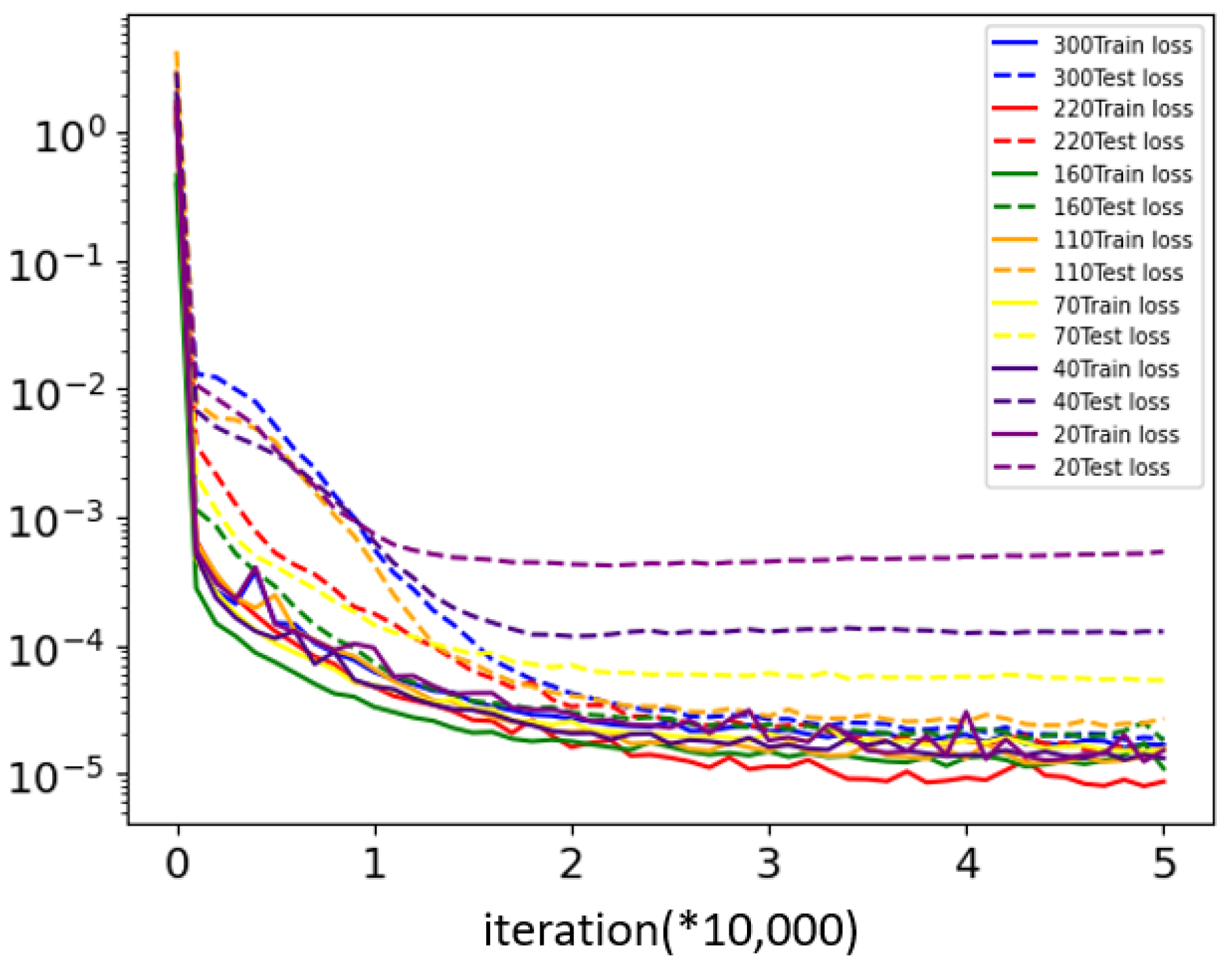
| Periods | Training Data Points | Functions | Discrete Points | Space | MSE |
|---|---|---|---|---|---|
| 6 | 20 | 200/40 | 20 × 20 | GRF | 1.17 × 10⁻³ |
| 6 | 40 | 200/40 | 20 × 20 | GRF | 1.24 × 10⁻⁴ |
| 6 | 70 | 200/40 | 20 × 20 | GRF | 5.36 × 10⁻⁵ |
| 6 | 110 | 200/40 | 20 × 20 | GRF | 2.43 × 10⁻⁵ |
| 6 | 160 | 200/40 | 20 × 20 | GRF | 1.81 × 10⁻⁵ |
| 6 | 220 | 200/40 | 20 × 20 | GRF | 1.59 × 10⁻⁵ |
| 6 | 300 | 200/40 | 20 × 20 | GRF | 1.84 × 10⁻⁵ |
| m | Data Points | Functions | MSE |
|---|---|---|---|
| 20 | 220 | 200/40 | 1.48 × 10⁻⁵ |
| 25 | 320 | 300/60 | 1.61 × 10⁻⁵ |
| 40 | 600 | 400/80 | 5.79 × 10⁻⁵ |
| 50 | 600 | 400/80 | 6.76 × 10⁻⁵ |
| Metrics | Our Method | CNN |
|---|---|---|
| Loss | 5.34 × 10⁻⁵ | 5.63 × 10⁻⁵ |
| Training time | 75 s | 348 s |
| Prediction time | 0.009 s | 0.03 s |
Disclaimer/Publisher’s Note: The statements, opinions and data contained in all publications are solely those of the individual author(s) and contributor(s) and not of MDPI and/or the editor(s). MDPI and/or the editor(s) disclaim responsibility for any injury to people or property resulting from any ideas, methods, instructions or products referred to in the content. |
© 2023 by the authors. Licensee MDPI, Basel, Switzerland. This article is an open access article distributed under the terms and conditions of the Creative Commons Attribution (CC BY) license (https://creativecommons.org/licenses/by/4.0/).
Share and Cite
Zhang, X.; Wang, Y.; Peng, X.; Zhang, C. An Efficient Method for Solving Two-Dimensional Partial Differential Equations with the Deep Operator Network. Axioms 2023, 12, 1095. https://doi.org/10.3390/axioms12121095
Zhang X, Wang Y, Peng X, Zhang C. An Efficient Method for Solving Two-Dimensional Partial Differential Equations with the Deep Operator Network. Axioms. 2023; 12(12):1095. https://doi.org/10.3390/axioms12121095
Chicago/Turabian StyleZhang, Xiaoyu, Yichao Wang, Xiting Peng, and Chaofeng Zhang. 2023. "An Efficient Method for Solving Two-Dimensional Partial Differential Equations with the Deep Operator Network" Axioms 12, no. 12: 1095. https://doi.org/10.3390/axioms12121095