New Partially Linear Regression and Machine Learning Models Applied to Agronomic Data

Abstract

Regression analysis can be appropriate to describe a nonlinear relationship between the response variable and the explanatory variables. This article describes the construction of a partially linear regression model with two systematic components based on the exponentiated odd log-logistic normal distribution. The parameters are estimated by the penalized maximum likelihood method. Simulations for some parameter settings and sample sizes empirically prove the accuracy of the estimators. The superiority of the proposed regression model over other regression models is shown by means of agronomic experimentation data. The predictive performance of the new model is compared with two machine learning techniques: decision trees and random forests. These methods achieved similar prediction performance, i.e., none stands out as a better predictor. In this sense, the objective of the research is to choose the best method. If the objective is only predictive, the decision tree can be used due to its simplicity. For inference purposes, the regression model is recommended, which can provide much more information regarding the relationship of the variables under study.

1. Introduction

Regression analysis is an important statistical tool to investigate the relationship between two or more variables. This relationship can be linear or nonlinear, which should be verified adequately. The incorrect assumption of linearity can compromise the reliability of the hypothesis tests and lead to poorly specified models. Semiparametric models are an interesting alternative for real data since they can access this relationship with more flexibility by means of nonparametric functions without imposing stringent conditions such as the commonly used nonlinear regression models. They enable the investigation of linear and nonlinear effects of the covariates simultaneously and can access this relationship. Because of these advantages, these models are receiving more attention in the literature.

Normal linear regression models are generally applied in different areas to model real data. However, it is known that several phenomena are not always in accordance with the normal model due to the lack of symmetry of the distribution or the presence of heavy tails. Another standard assumption in regression analysis is the homogeneity of error variability. Violation of this assumption may have adverse consequences for the efficiency of the estimators. Therefore, it becomes important to check heteroscedasticity. In this paper, we propose a partial linear regression model, where the mean and dispersion parameters vary across the observations through regression structures, assuming that the model response follows the exponentiated odd log-logistic normal (EOLLN) distribution. A special feature of this regression model is that it can model symmetric, asymmetric, and bimodal data.

Some models for nonparametric functions can be cited: a semiparametric model for the median and skewness [1], a skew-normal semiparametric model [2], an exponentiated sinh Cauchy model [3], and a log-sinh Cauchy model with cure fraction [4]. In the Bayesian context, the following can be cited: a semiparametric regression model in microbiology [5], a semiparametric model for tea productivity [6], an extended Maxwell semiparametric model [7], and an exponentiated power exponential regression [8].

Other alternatives that have been gaining popularity are machine learning models ([9,10,11,12]). Models based on decision trees (DTs) and random forests (RFs), which are nonlinear and nonparametric techniques, can be more flexible than the usual regression models. Since nonparametric methods are free of assumptions and do not require prior knowledge of the functional form of the relation between the response variable and the covariates, they are also robust to the presence of outliers and can be used with asymmetric data [13].

Articles related to plantain varieties are important for farmers, researchers, and professionals in the field. There are several variations of agronomic potential among varieties, which have been minimally explored ([14,15,16]). The knowledge of this potential can help to obtain more sustainable and profitable practices, which are the patterns of growth, a basic knowledge. Given the scarcity of these studies, we define a new regression model for the pseudostem height in the planting–flowering period of banana varieties.

Figure 1a displays the scatterplot between the pseudostem height and planting–flowering period, where these variables do not have a linear relationship. The second covariate related to the response variable is a variety (a factor with nine levels). The relationship of this variable with the response variables in Figure 1b shows that there is a heterogeneity of variances and several discrepant points (outliers). In view of these facts, two statistical tools may be appropriate.

First, a heterogeneous semiparametric partially linear regression model can be a suitable alternative. This model can adequately study the nonlinear relationship of the covariate period (continuous) with the response through nonparametric functions together with the linear effect of the covariate variety (factor). Further, we verify the effects of these covariates on the dispersion parameter.

Second, the DT and RF machine learning algorithms can be alternatives to predict the pseudostem height in terms of the covariates. The choice of these algorithms is based on their simplicity since they do not require prior knowledge of the functional form of the relation between these covariates and the response variable. Due to their easy interpretation and computational implementation, models based on decision trees are very attractive to researchers in areas other than statistics, although they are less precise than the usual regression models.

This article is summarized as follows. Section 2 defines the EOLLN distribution [17], which can model bimodal data and/or data with positive or negative asymmetry, and proposes a partially linear regression using P-splines based upon this distribution. The machine learning methodology is briefly addressed in Section 3. Some simulations are carried out in Section 4. The utility of the new regression model is illustrated through agronomic data in Section 5. Some conclusions are addressed in Section 6.

2. The EOLLN Model

The probability density function (pdf) of the EOLLN model is determined from [17] by taking the normal as baseline

$$\begin{array}{c}\hfill f\left(y\right)=f(y;\nu ,\tau ,\mu ,\sigma )=\frac{\nu \tau \varphi \left(\begin{array}{c}\frac{y-\mu }{\sigma }\end{array}\right){\left[\begin{array}{c}\mathsf{\Phi }\left(\begin{array}{c}\frac{y-\mu }{\sigma }\end{array}\right)\end{array}\right]}^{\nu \tau -1}{\left[\begin{array}{c}1-\mathsf{\Phi }\left(\begin{array}{c}\frac{y-\mu }{\sigma }\end{array}\right)\end{array}\right]}^{\nu -1}}{\sigma {\left\{\begin{array}{c}\mathsf{\Phi }{\left(\begin{array}{c}\frac{y-\mu }{\sigma }\end{array}\right)}^{\nu }+{\left[\begin{array}{c}1-\mathsf{\Phi }\left(\begin{array}{c}\frac{y-\mu }{\sigma }\end{array}\right)\end{array}\right]}^{\nu }\end{array}\right\}}^{\tau +1}},\end{array}$$

(1)

where $y\in \mathbb{R}$, $\mu \in \mathbb{R}$ is a location, $\sigma >0$ is a scale, and $\mathsf{\Phi }(·)$ and $\varphi (·)$ are the cumulative distribution function (cdf) and pdf of the standard normal, respectively.

Hereafter, let $Y\sim \mathrm{EOLLN}(\nu ,\tau ,\mu ,\sigma )$ be a random variable with density function (1). The three special EOLLN models are: OLLN [18] when $\tau =1$, exponentiated normal (Exp-N) [19]) when $\nu =1$, and clearly, normal when $\nu =\tau =1$.

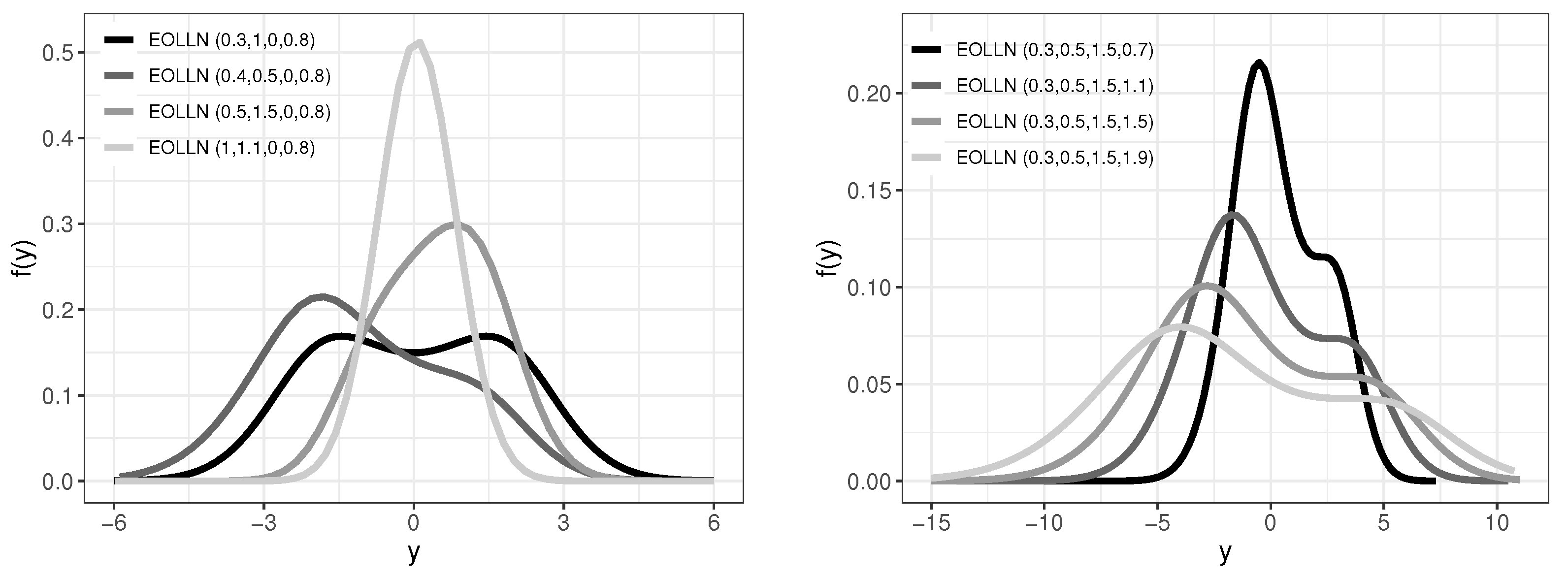
Figure 2 shows the flexibility of the EOLLN density such as bimodality and positive and negative asymmetry.

The quantile function (qf) of Y is given by (for $0<u<1$)

$$\begin{array}{c}\hfill Q\left(u\right)=Q_N\left\{\frac{u^{1/\left(\nu \tau \right)}}{u^{1/\left(\nu \tau \right)}+{(1-u^{1/\tau })}^{1/\nu }}\right\},\end{array}$$

(2)

where $Q_N(·)=G^{-1}(·;\mu ,\sigma )$ is the normal qf.

The EOLLN Partially Linear Regression Model

Consider independent observations $Y_1,\cdots ,Y_n$, and the systematic components (for $i=1,\dots ,n$)

$$g_1\left({\mu }_i\right)={\eta }_{i1}={{\mathit{x}}_{\mathit{i}\mathbf{1}}}^{\top }{\mathit{\beta }}_1,\mathrm{and}{g}_2\left({\sigma }_i\right)={\eta }_{i2}={{\mathit{x}}_{\mathit{i}\mathbf{2}}}^{\top }{\mathit{\beta }}_2,$$

(3)

where (for $k=1,2$) ${\mathit{x}}_{ik}={(1,x_{ik1},\cdots ,x_{ik{p}_k})}^{\top }$ is the explanatory variable vector, ${\mathit{\beta }}_k={({\beta }_{k0},\cdots ,{\beta }_{kp})}^{\top }$ is a $p_k+1$ vector of unknown coefficients, and ${\eta }_{ik}$ is the linear predictor. The strictly monotone functions $g_1$ and $g_2$ are defined from $\mathbb{R}\to \mathbb{R}$ and $\mathbb{R}\to {\mathbb{R}}^{+}$, respectively.

The logarithm of the likelihood function for $\mathit{\theta }={(\nu ,\tau ,{\mathit{\beta }}_1^{\top },{\mathit{\beta }}_2^{\top })}^{\top }$ can be expressed as

$$\begin{array}{ccc}\hfill l\left(\mathit{\theta }\right)& =& nlog\left(\frac{\nu \tau }{\sigma }\right)+\sum _{i=1}^{n}log\left[\varphi \left(\frac{y_i-{\mu }_i}{{\sigma }_i}\right)\right]+(\nu \tau -1)\sum _{i=1}^{n}log\left[\mathsf{\Phi }\left(\frac{y_i-{\mu }_i}{{\sigma }_i}\right)\right]+\hfill \\ & & (\nu -1)\sum _{i=1}^{n}log\left[1-\mathsf{\Phi }\left(\frac{y_i-{\mu }_i}{{\sigma }_i}\right)\right]-\hfill \\ & & (\tau +1)\sum _{i=1}^{n}log\left\{\mathsf{\Phi }{\left(\frac{y_i-{\mu }_i}{{\sigma }_i}\right)}^{\nu }+{\left[1-\mathsf{\Phi }\left(\frac{y_i-{\mu }_i}{{\sigma }_i}\right)\right]}^{\nu }\right\}.\hfill \end{array}$$

(4)

We maximize (4) using R (gamlss) [20] or (optim), SAS (Proc NLMixed). The initial coefficients are the values from the fitted normal regression.

The EOLLN partially linear regression model is constructed using P-splines [21] for the nonlinear effects, and changing Equations (3) by

$$g_1\left({\mu }_i\right)={\eta }_{i1}={{\mathit{x}}_{\mathit{i}\mathbf{1}}}^{\top }{\mathit{\beta }}_1+h\left(t_i\right),\mathrm{and}{g}_2\left({\sigma }_i\right)={\eta }_{i2}={{\mathit{x}}_{\mathit{i}\mathbf{2}}}^{\top }{\mathit{\beta }}_2,$$

(5)

where $h\left(t_i\right)$ is a smooth function of the explanatory variable $t_i$ in an interval $[a,b]$.

Let $\mathit{\omega }={({\mathit{\theta }}^{\top },{\mathit{h}}^{\top })}^{\top }$ be the full parameter vector, where $\mathit{h}={(h\left(t_1^0\right),\cdots ,h\left(t_q^0\right))}^{\top }$ is the vector of nonlinear effects. The maximum likelihood estimates (MLEs) are calculated by maximizing the penalized log-likelihood

$$\begin{array}{ccc}\hfill l_p\left(\mathit{\omega }\right)& =& l\left(\mathit{\theta }\right)-\frac{\lambda }{2}{\mathbf{h}}^{\top }\mathbf{K}\mathbf{h},\hfill \end{array}$$

(6)

where $l\left(\mathit{\theta }\right)$ is given by (4), $\lambda >0$ is the unknown smoothing parameter, and $\mathbf{K}$ is a symmetric matrix depending on smoothing parameters (for details, see [22]).

The total degrees of freedom of the model is the sum of the degrees of freedom adopted to all additive and parametric terms as reported in [23]. We use the Penalized Quasi-Likelihood (PQL) method [24] to estimate the smoothing parameters and the degrees of freedom of the P-Spline smooth functions. We use the RS algorithm implemented in the gamlss package in R to maximize (6). The function pb(·) assigns additive terms to explanatory variables. The PQL method is described in [25].

The residuals can identify the discrepancy between the fitted model and the data, and the construction of an envelope to better interpret them is reported in [26]. The quantile residuals (qrs) for the proposed regression model are

$$\begin{array}{c}\hfill {qr}_i={\mathsf{\Phi }}^{-1}\left\{\frac{{\mathsf{\Phi }}^{\widehat{\nu }\widehat{\tau }}\left(\frac{y_i-{\widehat{\mu }}_i}{{\widehat{\sigma }}_i}\right)}{{\left\{{\mathsf{\Phi }}^{\widehat{\nu }}\left(\frac{y_i-{\widehat{\mu }}_i}{{\widehat{\sigma }}_i}\right)+{\left[1-\mathsf{\Phi }\left(\frac{y_i-{\widehat{\mu }}_i}{{\widehat{\sigma }}_i}\right)\right]}^{\widehat{\nu }}\right\}}^{\widehat{\tau }}}\right\},\end{array}$$

(7)

where ${\mu }_i$ and ${\sigma }_i$ follow from Equation (5).

3. Machine Learning Methods

Machine learning is a sub-area of artificial intelligence. It involves supplying machines with data so that they learn and are able to predict new results when new data are presented. In this process, different models are fitted to a dataset (training dataset), applied to a validation dataset (or testing dataset), and compared according to a performance criterion with the objective of forecasting future units. In traditional regression analysis, the goal is also to study the relationship between the variables, while assuming that the available data belong to a random sample.

There are two classes of machine learning: supervised and unsupervised. In the first class, predictor variables are used to forecast one or more response variables (called labeled variables). For qualitative responses, this problem is known as classification, while for quantitative responses it is called prediction. In turn, in unsupervised learning, all of the variables of the dataset are considered without distinction between predictor and response variables, and the objective is to describe associations and patterns among them. This study is focused on regression problems using two supervised algorithms, as described below.

3.1. Decision Trees

The use of decision trees is a nonparametric method that leads to easily interpreted results. The tree is constructed by recursively subdividing the space generated by the predictor variables. Each partition is called a node and each final result is called a leaf (terminal node). This method is based on Classification and Regression Trees (CARTs) [27], according to the following strategy:

1.

Partition the space generated by the predictor variables ($X_1,\cdots ,X_p$) into m regions $R_1,\cdots ,R_m$.

2.

For each element belonging to $R_j$, the predictor of Y (called ${\widehat{Y}}_{R_j}$) will be the mean between the points with values of $X_1,\cdots ,X_p$ in $R_j$.

However, the division into many partitions is computationally unfeasible, and besides this, multiple divisions can rapidly fragment the data, making the dataset insufficient for the next levels and hampering the learning of the algorithm. In light of this situation, the decision tree algorithm utilizes a recursive binary splitting (top-down) approach. If the optimality criterion is to minimize the sum of the square errors (SSE), the steps follow as:

1.

Let the predictor variables $X_j$ and their possible cutoff points be t, and consider the regions, for all pairs $(j,t)$,

$$R_1(j,t)=\{\mathit{X}:X_j<t\},R_2(j,t)=\{\mathit{X}:X_j\ge t\}.$$

2.

Select the pair $(j,t)$ that gives the smallest SSE:

$$\mathrm{SSE}=\sum _{i:x_i\in R_1(j,t)}{(y_i-{\widehat{y}}_{i{R}_1})}^2+\sum _{i:x_i\in R_2(j,t)}{(y_i-{\widehat{y}}_{i{R}_2})}^2.$$

3.

Repeat the procedure only with the data partition until some criterion is satisfied (e.g., obtaining a fixed minimum number of elements in each region).

One of the problems associated with decision trees is overfitting, which consists of obtaining the terminal nodes equal to the number of observations, i.e., each element of the dataset used is perfectly predicted. The pruning of the trees can resolve this problem, generating fewer nodes with lower variance and greater interpretability, although this can slightly increase the bias. A way to prune the tree is to examine the complexity parameter (CP), which serves to control the size of the tree and corresponds to the smallest increment in the cost of the model necessary to consider a new subdivision. In general, the goal is to find the level for which the CP is minimized.

3.2. Random Forests

Random forests (RFs) [28] are generalizations of models based on trees with the objective of reducing the variability and bias [29] by the insertion of two forms of randomness in their construction. Various trees are constructed with different bootstrap samples of the data and each tree is cultivated using a random subset of predictor variables. The trees are cultivated without pruning and all of the responses of individual trees are combined by the average to obtain the forecasts of the final output. This combination of results characterizes the algorithm as an ensemble and can be more precise than any single-constituent model. The RF classifies the predictor variables in decreasing order and evaluates them simultaneously, but it behaves like a “black box”, because the trees cannot be examined separately ([30,31]).

Start with a training set with n elements, $({\mathit{x}}_i,y_i)$, $i=1,\dots ,n$, where ${\mathit{x}}_i$ is a vector of p predictor variables associated with the ith response variable. Consider the following steps:

1.

Obtain B bootstrap samples with a replacement of size n based on the training data. In general, the number of elements chosen in each sample is the order $2/3$ of the n elements of the set provided for training. The remaining elements are called out-of-bag (OOB) samples;

2.

Select $m<p$ predictor variables randomly;

3.

In the construction of each node of the tree, choose the best predictor among the selected m;

4.

For each unpruned tree, determine the predictor of Y, ${\widehat{y}}^b\left(\mathit{x}\right)$, where $b=1,\dots ,B$;

5.

Aggregate all of the predictors as ${\widehat{y}}_{RF}^B\left(\mathit{x}\right)=\frac{1}{B}{\sum }_{b=1}^B{\widehat{y}}^b\left(\mathit{x}\right)$.

3.3. Cross-Validation

Cross-validation has the objective of avoiding problems like overfitting and bias, and of verifying the capacity for the generalization of a model, i.e., its prediction performance with new data. The aforementioned division of the dataset into two disjoint subsets (training and testing) is the simplest cross-validation technique, called hold-out. Since the partition is performed randomly, high variability can be obtained depending on the training set utilized. The k-fold method [32] can be an interesting alternative.

In this method, n observations from the original sample $\mathcal{D}$ are divided into K disjoint subsets of observations, namely ${\mathcal{D}}_1,\cdots ,{\mathcal{D}}_K$, each one having approximately equal size $m_k$ such that $n={\sum }_{k=1}^K{m}_k$. The validation sample is composed of the partition ${\mathcal{D}}_k$, while the training sample consists of the other $K-1$ partitions not including the kth partition, i.e., the training set is given by ${\mathcal{D}}_{(-k)}=\{{\mathcal{D}}_1,\cdots ,{\mathcal{D}}_{k-1},{\mathcal{D}}_{k+1},\cdots ,{\mathcal{D}}_K\}$. This process is repeated iteratively K times until each of $k=1,\dots ,K$ partitions is considered a validation sample. A general recommendation is to use $K=5$ or $K=10$, where greater values of K imply larger training samples, and, hence, greater variances and higher computational costs, but can also generate smaller biases [33].

4. Simulation Study

A Monte Carlo simulation study (for sample sizes n = 50, 150, and 450) evaluates the consistency of the estimates in the proposed regression model, and the empirical distribution of the qrs is determined by the RS algorithm in the gamlss package. We generate r = 1000 samples from Equation (2) with two covariates $x_1\sim \mathrm{Binomial}(1,0.5)$ and $t\sim \mathrm{Uniform}(0,1)$ under two scenarios:

Scenario 1 (homogeneous variance and cubic relationship): The first systematic component is $\mu ={\beta }_{11}{x}_{1i}+h\left(t_i\right)$, where $h\left(t_i\right)=2t_i+sin\left(2\pi t_i\right)$ to obtain a cubic relationship. The true values for the generation process are ${\beta }_{11}=0.4$, $log\left(\sigma \right)=-1.6$, $log\left(\nu \right)=0.5$ and $log\left(\tau \right)=0.6$.

Scenario 2 (heterogeneous variance and quadratic relationship): The second systematic component is $\mu ={\beta }_{11}{x}_{1i}+h\left(t_i\right)$ and $\sigma =exp({\beta }_{20}+{\beta }_{21}{x}_{1i}+{\beta }_{22}{t}_i)$, respectively, where $h\left(t_i\right)=sin\left(\pi t_i\right)$ to obtain a quadratic relationship. The true values in the generation process are ${\beta }_{11}=0.6$, ${\beta }_{20}=-1.3$, ${\beta }_{21}=1.1$, ${\beta }_{22}=0.9$, $log\left(\nu \right)=0.4$ and $log\left(\tau \right)=0.5$.

The following steps are carried out:

(i)

Obtain $x_{1i}\sim \mathrm{Binomial}(1,0.5)$ and $t_i\sim \mathrm{Uniform}(0,1)$;

(ii)

Calculate $\mu$ and $\sigma$ from their respective systematic components in each scenario;

(iii)

Set $u_i\sim \mathrm{Uniform}(0,1)$;

(iv)

Calculate the observations from Equation (2) using the previous steps;

(v)

Determine the qrs.

The average estimates (AEs), biases, and mean squared errors (MSEs) are found for each replication.

Table 1. Findings from the simulated new regression model.

Scenario 1		n = 50			n = 150			n = 450
$\mathit{\omega }$	True	AEs	Biases	MSEs	AEs	Biases	MSEs	AEs	Biases	MSEs
${\beta }_{11}$	0.4	0.40	−0.00	0.00	0.40	−0.00	0.00	0.40	−0.00	0.00
$log\left(\sigma \right)$	−1.6	−1.71	−0.11	0.04	−1.64	−0.04	0.01	−1.62	−0.02	0.00
$log\left(\nu \right)$	0.5	0.54	0.04	0.04	0.51	0.01	0.00	0.50	0.00	0.00
$log\left(\tau \right)$	0.6	0.63	0.03	0.15	0.61	0.01	0.02	0.61	0.01	0.00
Scenario 2		n = 50			n = 150			n = 450
$\mathit{\omega }$	True	AEs	Biases	MSEs	AEs	Biases	MSEs	AEs	Biases	MSEs
${\beta }_{11}$	0.6	0.59	−0.01	0.04	0.59	−0.01	0.01	0.60	−0.00	0.00
${\beta }_{20}$	−1.3	−1.50	−0.20	0.15	−1.37	−0.07	0.03	−1.32	−0.02	0.01
${\beta }_{21}$	1.1	1.21	0.11	0.08	1.13	0.03	0.02	1.11	0.01	0.01
${\beta }_{22}$	0.9	0.96	0.06	0.20	0.92	0.02	0.05	0.90	0.00	0.02
$log\left(\nu \right)$	0.4	0.40	−0.00	0.03	0.40	−0.00	0.01	0.39	−0.01	0.00
$log\left(\tau \right)$	0.5	0.53	0.03	0.11	0.52	0.02	0.02	0.50	0.00	0.01

confirms that the AEs converge to the true parameters and the biases and the MSEs decay if n increases. So, the estimators are consistent. The plots in Figure 3 and Figure 4 reveal that the generated smoothed curves approximate the true curve when n increases, i.e., the estimator of the nonparametric part is also consistent. We emphasize that the quadratic and cubic forms are only used to illustrate possible relationships between variables. The model has the flexibility to accommodate different nonlinear relationships without the need to restrictively define its format. The normal probability plots in Figure 5 and Figure 6 reveal that the empirical distribution of the qrs tends to the standard normal distribution.

Predictive Performance

For Scenarios 1 and 2, we verify the predictive capacity of the EOLLN model, decision trees, and random forests. Each of the 1000 samples is divided into training and validation sub-samples, BY approximately 70% and 30%, respectively. The models are fitted to the training data, and the coefficient of determination (R${}^2$), root mean square error (RMSE), and variance accounted for (VAF) are calculated using the test data. The coefficient R${}^2$ evaluates the accuracy of the model fitting with values between 0 and 1, where the higher values mean the stronger explanatory power. The RMSE indicates the prediction errors, i.e., it shows discrepancies between predicted and observed values, where values closer to zero are considered adequate. The VAF is typically adopted to verify if the predictive model is rigorous [34]. The more accurate the prediction is, the VAF of the predictive model will be closer to 100 (i.e., lower variance). These metrics are:

$${\mathrm{R}}^2=\frac{{\sum }_{i=1}^n{y}_i^2-{\sum }_{i=1}^n{(y_i-{\widehat{y}}_i)}^2}{{\sum }_{i=1}^n{y}_i^2},$$

(8)

$$\mathrm{RMSE}={\left[\frac{1}{n}\sum _{i=1}^n{(y_i-\widehat{y_i})}^2\right]}^{1/2},$$

(9)

$$\mathrm{VAF}=100\times \left[1-\frac{var(y_i-\widehat{y_i})}{var\left(y_i\right)}\right],$$

(10)

where $y_i$’s are the observed values for the validation set, n is its size, and ${\widehat{y}}_i$’s are the predicted values.

These values can be noted in the boxplots for the 1000 replicates of each sample size in Figure 7, Figure 8 and Figure 9. The results are given below:

• All models perform worse for Scenario 2, which can be justified by the presence of heterogeneous variance;
• All metrics improve for larger sample sizes, for all models, and in both scenarios;
• For the first scenario, better performance of the EOLLN regression model is notable, i.e., higher R${}^2$s, lower RMSEs, and higher VAFs;
• On the other hand, for the second scenario, we can observe similar results for both models.

5. Application: Pseudostem Height Data

Consider a dataset from a homogeneous experimental design of 3000 m${}^2$ conducted in the African Center for Banana and Plantain Researches (CARBAP) experimental station in Cameroon by plantain researchers, where nine varieties of plantain-like hybrids are found interesting and promising based on characteristics such as the structure of the bunch or tolerance to disease; they are: Batard (BA)—Natural and Giant; Big Ebanga (BE)—Natural and Medium; CRBP39 (CR)—Hybrid-a and Medium; D248 (DD)—Hybrid-a and Medium; D535 (DC)—Hybrid-a and Medium; Essong (ES)—Natural and Giant; French Clair (FC)—Natural and Medium; FHIA21 (FH)—Hybrid-b and Medium; and Mbouroukou no. 3 (MB)—Natural and Medium, where hybrid-a was obtained from the CIRAD-CARBAP breeding collaborative program and hybrid-b from the FHIA breeding program.

The experiment was conducted from the plantation (on 29 July 2009) on the harvest of the first crop cycle of each variety; the last mother plants were harvested in February 2011. So, this is mostly mother-plant data.

The completely randomized experimental design described in [35] has the pseudostem height as the response and variety as a single factor. Five replicates of each variety were considered, totaling 45 plants per variety. Cropping conditions such as mineral nutrition, fertilization, and irrigation are not taken into account. The pseudostem height was measured between the soil and the bottom of the “V” formed by the two leaves last emitted in the stage “complete flowering” or “flowering”, i.e., the day when the latest fertile hand has appeared. The dataset includes $n=355$ observations of height, so not all varieties have records of the flowering period. So, the variables under study are:

• $y_i$: pseudostem height (in cm);
• $t_i$: planting–flowering period (in days);
• $x_{i1}$: varieties ($i=1,\dots ,355$).

The covariate $x_{i1}$ has nine levels, and then eight dummy variables ($d_{ij}$, $j=1,\dots 8$) are defined.

Complementing the descriptive analysis shown in the introduction (Figure 1), Figure 10 displays the scatter plot of the pseudostem height as a function of days per variety. The varieties achieved complete flowering on different days, especially the ES variety.

5.1. The EOLLN Partially Linear Regression Model

The proposed regression model is compared with three sub-models (OLLN, Exp-N, and Normal) and the partially linear regression model based on the skew-normal distribution [2], whose pdf is ($y\in \mathbb{R}$)

$$\begin{array}{c}\hfill f(\mu ,\sigma ,\nu )=\frac{2}{\sigma }\varphi \left(\begin{array}{c}\frac{y-\mu }{\sigma }\end{array}\right)\mathsf{\Phi }\left(\begin{array}{c}\nu \frac{y-\mu }{\sigma }\end{array}\right),\end{array}$$

(11)

where $\mu \in \mathbb{R}$, $\sigma >0$ and $\nu \in \mathbb{R}$.

The following systematic components are defined (for $i=1,\dots ,355$):

$$\begin{array}{c}\hfill {\mu }_i={\beta }_{10}+\sum _{j=1}^8{\beta }_{1j}{d}_{ij}+h\left(t_i\right)\mathrm{and}{\sigma }_i=exp\left({\beta }_{20}+\sum _{j=1}^8{\beta }_{2j}{d}_{ij}\right).\end{array}$$

(12)

Note that the covariate $x_1$ (varieties) has nine levels (BA, BE, CR, DC, DD, ES, FC, FH, MB). Then, we create eight dummy variables $(d_1,\cdots ,d_8)$ taking the first level of the BA variety as a reference. For example, the dummy variable $d_1$ measures the effect of the BA variety level in relation to the BE level. The other dummy variables have similar interpretations.

Two well-known statistics (denoted by acronyms) and the global deviance (GD) are reported in

Table 2. Adequacy measures.

Model	AIC	BIC	GD
EOLLN	3244.21	3339.18	3195.17
OLLN	3262.07	3349.77	3216.77
Exp-N	3258.24	3339.55	3216.24
Normal	3285.22	3362.66	3245.22
Skew-Normal	3287.28	3368.60	3245.28

. The new regression model gives the lowest values of these statistics, and then it can be chosen as the most appropriate to explain the pseudostem height. The likelihood ratio (LR) test for nested models provides p-values $<0.001$, thus confirming our findings.

We move up to the analysis from the fitted EOLLN partially linear regression model, where the maximum likelihood estimates (MLEs), standard errors (SEs), and p-values are given in

Table 3. Findings from the new fitted regression model.

$\mathit{\omega }$	MLEs	SEs	p-Values	$\mathit{\omega }$	MLEs	SEs	p-Values
${\beta }_{10}$	399.1348	13.0847	<$0.01$	${\beta }_{20}$	3.2329	0.4815	<$0.01$
${\beta }_{11}$	−46.6931	5.6440	<$0.01$	${\beta }_{21}$	0.2657	0.1917	0.1667
${\beta }_{12}$	−80.6066	5.4382	<$0.01$	${\beta }_{22}$	0.3085	0.2379	0.1955
${\beta }_{13}$	−50.6933	6.0629	<$0.01$	${\beta }_{23}$	0.4544	0.2568	0.0776
${\beta }_{14}$	−133.6910	4.7972	<$0.01$	${\beta }_{24}$	−0.2778	0.2134	0.1939
${\beta }_{15}$	11.3575	4.5705	0.0134	${\beta }_{25}$	−0.7994	0.2888	<$0.01$
${\beta }_{16}$	−73.0926	5.0582	<$0.01$	${\beta }_{26}$	0.1906	0.2222	0.3916
${\beta }_{17}$	−104.5167	4.8448	<$0.01$	${\beta }_{27}$	−0.0084	0.2068	0.9674
${\beta }_{18}$	−42.5077	4.9276	<$0.01$	${\beta }_{28}$	0.0087	0.1826	0.9621
				$log\left(\nu \right)$	1.9281	0.0447	<$0.00001$
				$log\left(\tau \right)$	−0.7528	0.0493	<$0.00001$

. The nonlinear effects ($t_i$) will be interpreted at the end through Figure 11a. Figure 11 shows the partial effects of the day variable on the parameters $\mu$ and $\sigma$. We conclude that the average of the pseudostem height is constant until (approximately) day 300. After this day, this average grows as the days go by; see Figure 11a. The variability of the pseudostem height grows when the days pass; see Figure 11b.

The qrs for the fitted regression models are compared by worm plots in Figure 12, thus supporting that our proposal yields the best fit. Figure 13 shows that the qrs are randomly distributed around zero and the majority of them are in the interval [−3,3]. In turn, Figure 13b indicates that nearly all points are within the simulated envelope. So, the new regression model is adequate. Further, Figure 14 provides the histograms with the marginally adjusted densities, and Figure 14b displays the estimated and empirical cumulative functions for each level of the variety. Hence, the proposed regression model suitably captures the distribution of this response variable.

Finally, some conclusions can be inferred from Table 3:

• Interpretations for $\mu$:

  -

  All varieties are significant in terms of mean pseudostem height compared to BA variety.

  -

  Only the ES variety (${\beta }_{15}$) has positive effects in relation to the BA variety, i.e., its mean is higher. Therefore, the other varieties have negative effects.

  -

  From

  Table 4. Comparing varieties according to the new regression model.

  Hypotheses ${\mathit{H}}_0$	Tests for the Location $\mathit{\mu }$			Tests for the Scale $\mathit{\sigma }$
  	MLEs	SEs	p-Values	MLEs	SEs	p-Values
  BE-BA	−46.693	5.644	<$0.01$	0.266	0.192	0.167
  CR-BA	−80.607	5.438	<$0.01$	0.309	0.238	0.195
  DC-BA	−50.693	6.063	<$0.01$	0.454	0.257	0.078
  DD-BA	−133.691	4.797	<$0.01$	−0.278	0.213	0.194
  ES-BA	11.357	4.570	0.013	−0.799	0.289	<$0.01$
  FC-BA	−73.093	5.058	<$0.01$	0.191	0.222	0.392
  FH-BA	−104.517	4.845	<$0.01$	−0.008	0.207	0.967
  MB-BA	−42.508	4.928	<$0.01$	0.009	0.183	0.962
  CR-BE	−33.913	5.194	<$0.01$	0.043	0.203	0.833
  DC-BE	−4.000	6.011	0.506	0.189	0.232	0.417
  DD-BE	−86.998	4.476	<$0.01$	−0.543	0.174	<$0.01$
  ES-BE	58.051	5.943	<$0.01$	−1.065	0.316	<$0.01$
  FC-BE	−26.399	5.046	<$0.01$	−0.075	0.192	0.696
  FH-BE	−57.824	5.017	<$0.01$	−0.274	0.180	0.128
  MB-BE	4.185	5.009	0.404	−0.257	0.141	0.070
  DC-CR	29.913	5.615	<$0.01$	0.146	0.266	0.584
  DD-CR	−53.084	3.854	<$0.01$	−0.586	0.213	<$0.01$
  ES-CR	91.964	5.862	<$0.01$	−1.108	0.364	<$0.01$
  FC-CR	7.514	4.580	0.102	−0.118	0.231	0.610
  FH-CR	−23.910	4.596	<$0.01$	−0.317	0.224	0.158
  MB-CR	38.099	4.563	<$0.01$	−0.300	0.191	0.116
  DD-DC	−82.998	4.956	<$0.01$	−0.732	0.245	<$0.01$
  ES-DC	62.051	6.356	<$0.01$	−1.254	0.357	<$0.01$
  FC-DC	−22.399	5.485	<$0.01$	−0.264	0.258	0.307
  FH-DC	−53.823	5.463	<$0.01$	−0.463	0.248	0.063
  MB-DC	8.186	5.453	0.134	−0.446	0.223	0.046
  ES-DD	145.048	5.295	<$0.01$	−0.522	0.348	0.135
  FC-DD	60.598	3.746	<$0.01$	0.468	0.206	0.024
  FH-DD	29.174	3.776	<$0.01$	0.269	0.198	0.174
  MB-DD	91.183	3.731	<$0.01$	0.286	0.159	0.073
  FC-ES	−84.450	5.379	<$0.01$	0.990	0.336	<$0.01$
  FH-ES	−115.874	5.074	<$0.01$	0.791	0.312	0.012
  MB-ES	−53.865	5.204	<$0.01$	0.808	0.316	0.011
  FH-FC	−31.424	4.366	<$0.01$	−0.199	0.212	0.348
  MB-FC	30.585	4.359	<$0.01$	−0.182	0.180	0.313
  MB-FH	62.009	4.300	<$0.01$	0.017	0.168	0.919

  , referring to the multiple comparisons, we note that there is no significant difference between the varieties DC-BE, FC-CR, and MB-DC for a 5% significance level. For other varieties, there is a significant difference. These results can be visualized graphically in Figure 14b.

• Interpretations for $\sigma$:

  -

  Only the ES variety (${\beta }_{25}$) is significant at a 5% level of significance, i.e., its variability differs from the BA variety.

  -

  From the multiple comparisons in Table 4, it is noted that there is a significant difference between the DD-BE, ES-BE, DD-CR, ES-CR, DD-DC, ES-DC, MB-DC, FC-DD, FC-ES, FH-ES, and MB-ES varieties in relation to the pseudostem height variability for a 5% significance level. For other varieties, there is no significant difference.

  -

  Again, these results are consistent with the descriptive analysis.

Table Table 4 reveals comparisons between all varieties from which similar interpretations to these can be made.

5.2. Machine Learning Models

The R software is also employed for the machine learning models. The decision trees are found with the rpart function of the rpart package and the random forests with the randomForest function of the randomForest package by defining the hyperparameters ntree = 500 and mtry = 1. The argument ntree denotes the number of trees to be cultivated in the forest, and mtry is the number of predictor variables to be considered in the construction of each node in the tree.

We perform the cross-validation method, described in Section 3.3, for $K=5$ and $K=10$. The K partitions are generated and the DT, RF, and EOLLN partially linear regression models are fitted to the training set.

For each model and K value, the average performance metrics (Equations (8)–(10)) are reported in

Table 5. Predictive performance of the EOLLN models, decision tree, and random forest according to the metrics: R${}^2$, RMSE, and VAF.

Model	RMSE	R${}^2$	VAF	Model	RMSE	R${}^2$	VAF
DT ($K=5$)	25.395	0.763	76.75	DT ($K=10$)	25.672	0.752	75.918
RF ($K=5$)	26.055	0.749	75.535	RF ($K=10$)	25.977	0.742	74.904
EOLLN ($K=5$)	29.089	0.683	76.359	EOLLN ($K=10$)	28.667	0.685	76.714

, from which the results follow:

1.

Regression model × machine learning models: there are small improvements of the DT and RF models regarding R${}^2$ and RMSE, but no improvement with regard to VAF;

2.

DT × RF: comparison of the two machine learning models reveals no significant improvements when changing from DT to RF;

3.

$K=5\times K=10$: with regard to the values of K, no significant difference occurred in the values of these metrics.

For both comparisons, these only slightly varying results can be related to the small number of covariates. The values of p and n influence the performance of the machine learning models, as noted by [36], who studied the performance of the models based on trees according to the sizes of these quantities.

The OOB error rates stabilized quickly, i.e., with a few trees for both values of K. This fact is again related to the small number of covariates, since one of the forms of randomness of the algorithm is to consider arbitrary variables at each node of the tree. An interesting result that can be obtained with RF is the importance plot. An increase in the percentage of the mean squared error (MSE) indicates greater importance. Figure 15 shows the importance of the variables planting–flowering days and varieties in terms of plantain pseudostem height. It can be seen that the variable variety is most important in predicting pseudostem height.

Further, we fit the complete decision tree model shown in Figure 16. Each node of the tree indicates the corresponding value of its function and the percentage of data in that node. The initial node gives the general average of the response variable. The need for pruning through the CP is checked, but it turns out not necessary in practice. We obtain six decision rules:

1.

If varieties = DD or FH and days < 236 then ${\widehat{y}}_i=304.1667$;

2.

If varieties = DD or FH and days ≥ 236 then ${\widehat{y}}_i=329.8936$;

3.

If varieties = CR or FC then ${\widehat{y}}_i=358.9438$;

4.

If varieties = BE or DC or MB then ${\widehat{y}}_i=388.6283$;

5.

If varieties = BA or ES and days < 369.5 then ${\widehat{y}}_i=440.5636$;

6.

If varieties = BA or ES and days ≥ 369.5 then ${\widehat{y}}_i=496.9333$.

We note that these rules agree with the descriptive analysis of the data. The scatterplot in Figure 10 shows that these rules hold for the variables and values of the days. Figure 14b also shows the agreement between the rules and the empirical cumulative functions of the varieties.

The objectives of the two proposed methods are very different, so the researcher’s purpose should be considered in choosing the best model. If the objective is to make predictions, the decision tree model can be the best, since it is much simpler. The decision rules for the prediction can be obtained easily and consulted rapidly. The RF is not recommended due to its greater complexity and absence of significant improvement in relation to the DT.

On the other hand, for researchers interested in making inferences along with predictions, we recommend the proposed regression model. The EOLLN partially linear regression model has the potential to supply information with regard to the variables studied, unlike the machine learning model. Besides this, it obtains equally satisfactory prediction results, so it can be used for both objectives.

6. Conclusions

This paper introduced a new partially linear regression model with the exponentiated odd log-logistic normal (EOLLN) distribution. It was motivated by an agronomic experiment involving banana varieties, where a nonlinear relationship occurred between the days from planting–flowering and the height of the pseudostem (response variable). Further, we noted heterogeneous variances for the covariable plant variety. The new EOLLN partially linear regression model was a suitable alternative to study the nonlinear relationship between the variables through nonparametric functions, and also to verify the effect of the variability of the varieties on the plant height through the parameter related to the variance of the distribution. We compared its predictive capacity with two machine learning algorithms: decision trees and random forests.

Additionally, the machine learning models were interesting alternatives to predict the response variable, because they did not need prior knowledge of the functional form between the response variable and the covariates. All of the methods obtained similar prediction performance, i.e., none stood out as the best predictor. The random forests achieved a stable OOB error rate with only a few trees, and the covariable variety stood out as the most important predictor of the plantain pseudostem height. However, although it is more robust than the decision tree model, it did not obtain better results regarding the predictive capacity of new values.

In this respect, for those wanting to make predictions, the decision tree model is recommended due to its simplicity. In turn, for researchers wanting to make inferences, we recommend the new regression model, which provides more information regarding the relationship of the variables under consideration, besides also having good prediction performance. The EOLLN partially linear regression model provides good inferences such as which varieties are significant regarding the mean and variance of the response, besides comparisons between the varieties, i.e., which of them differs from each other.

We carried out a simulation study under two scenarios that supply cubic and quadratic relations between the variables. The results showed that the new regression model was adequate to capture different nonlinear forms and provided consistent maximum likelihood estimators (MLEs).

In future works, we recommend analyzing other banana plant response variables due to the scarcity of studies related to this plant. We also suggest this model to analyze other datasets and problems in other areas of knowledge, where variables have a nonlinear relationship or the response variable is bimodal and/or skewed. Finally, we suggest comparing the new model with those of the machine learning methods to analyze datasets with a larger number of covariates (high-dimensional datasets).

References

- Vanegas, L.H.; Paula, G.A. A semiparametric approach for joint modeling of median and skewness. Test 2015, 24, 110–135. [Google Scholar] [CrossRef]
- Xu, D.; Zhang, Z.; Du, J. Skew-normal semiparametric varying coefficient model and score test. J. Stat. Comput. Simul. 2015, 85, 216–234. [Google Scholar] [CrossRef]
- Ramires, T.G.; Ortega, E.M.M.; Hens, N.; Cordeiro, G.M.; Paula, G.A. A flexible semiparametric regression model for bimodal, asymmetric and censored data. J. Appl. Stat. 2018, 45, 1303–1324. [Google Scholar] [CrossRef]
- Ramires, T.G.; Hens, N.; Cordeiro, G.M.; Ortega, E.M.M. Estimating nonlinear effects in the presence of cure fraction using a semi-parametric regression model. Comput. Stat. 2018, 33, 709–730. [Google Scholar] [CrossRef]
- Lee, J.; Sison-Mangus, M. A Bayesian semiparametric regression model for joint analysis of microbiome data. Front. Microbiol. 2018, 9, 522. [Google Scholar] [CrossRef] [PubMed]
- Dhekale, B.S.; Sahu, P.K.; Vishwajith, K.P.; Mishra, P.; Narsimhaiah, L. Application of parametric and nonparametric regression models for area, production and productivity trends of tea (Camellia sinensis) in India. Indian J. Ecol. 2017, 44, 192–200. [Google Scholar]
- Prataviera, F.; Ortega, E.M.M.; Cordeiro, G.M. An extended Maxwell semiparametric regression for censored and uncensored data. Commun. Stat.-Simul. Comput. 2023, 52, 3305–3326. [Google Scholar] [CrossRef]
- Prataviera, F.; Ortega, E.M.M.; Cordeiro, G.M.; Cancho, V.G. The exponentiated power exponential semiparametric regression model. Commun. Stat.-Simul. Comput. 2022, 51, 5933–5953. [Google Scholar] [CrossRef]
- Alonso, L.; Renard, F. A new approach for understanding urban microclimate by integrating complementary predictors at different scales in regression and machine learning models. Remote Sens. 2020, 12, 2434. [Google Scholar] [CrossRef]
- Oukawa, G.Y.; Krecl, P.; Targino, A.C. Fine-scale modeling of the urban heat island: A comparison of multiple linear regression and random forest approaches. Sci. Total Environ. 2022, 815, 152836. [Google Scholar] [CrossRef]
- Khan, M.A.; Shah, M.I.; Javed, M.F.; Khan, M.I.; Rasheed, S.; El-Shorbagy, M.A.; El-Zahar, E.R.; Malik, M.Y. Application of random forest for modelling of surface water salinity. Ain Shams Eng. J. 2022, 13, 101635. [Google Scholar] [CrossRef]
- Subeesh, A.; Bhole, S.; Singh, K.; Chandel, N.S.; Rajwade, Y.A.; Rao, K.V.R.; Kumar, S.P.; Jat, D. Deep convolutional neural network models for weed detection in polyhouse grown bell peppers. Artif. Intell. Agric. 2022, 6, 47–54. [Google Scholar] [CrossRef]
- Kuhn, M.; Johnson, K. Applied Predictive Modeling; Springer: New York, NY, USA, 2013; Volume 26, p. 13. [Google Scholar]
- Swennen, R.; Vuylsteke, D.; Ortiz, R. Phenotypic diversity and patterns of variation in West and Central African plantains (Musa spp., AAB group Musaceae). Econ. Bot. 1995, 45, 320–327. [Google Scholar] [CrossRef]
- Ortiz, R.; Madsen, S.; Vuylsteke, D. Classification of African plantain landraces and banana cultivars using a phenotypic distance index of quantitative descriptors. Theor. Appl. Genet. 1998, 96, 904–911. [Google Scholar] [CrossRef]
- Depigny, S.; Lescot, T.; Achard, R.; Diouf, O.; Côte, F.X.; Fonbah, C.; Sadom, L.; Tixier, P. Model-based benchmarking of the production potential of plantains (Musa spp., AAB): Application to five real plantain and four plantain-like hybrid varieties in Cameroon. J. Agric. Sci. 2017, 155, 888–901. [Google Scholar] [CrossRef]
- Alizadeh, M.; Tahmasebi, S.; Haghbin, H. The exponentiated odd log-logistic family of distributions: Properties and applications. J. Stat. Model. Theory Appl. 2020, 1, 29–52. [Google Scholar]
- Gleaton, J.U.; Lynch, J.D. Properties of generalized log-logistic families of lifetime distributions. J. Probab. Stat. Sci. 2006, 4, 51–64. [Google Scholar]
- Mudholkar, G.S.; Srivastava, D.K.; Kollia, G. A generalization of the Weibull distribution with application to the analysis of survival data. J. Am. Stat. Assoc. 1996, 91, 1575–1583. [Google Scholar] [CrossRef]
- R Core Team. R: A Language and Environment for Statistical Computing; R Foundation for Statistical Computing: Vienna, Austria, 2022. [Google Scholar]
- Eilers, P.H.; Marx, B.D. Flexible smoothing with B-splines and penalties. Stat. Sci. 1996, 11, 89–121. [Google Scholar] [CrossRef]
- Rigby, R.A.; Stasinopoulos, D.M. Generalized additive models for location, scale and shape. J. R. Stat. Soc. Ser. C Appl. Stat. 2005, 54, 507–554. [Google Scholar] [CrossRef]
- Voudouris, V.; Gilchrist, R.; Rigby, R.; Sedgwick, J.; Stasinopoulos, D. Modelling skewness and kurtosis with the BCPE density in GAMLSS. J. Appl. Stat. 2012, 39, 1279–1293. [Google Scholar] [CrossRef]
- Lee, Y.; Nelder, J.A.; Pawitan, Y. Generalized Linear Models with Random Effects: Unified Analysis via H-Likelihood; Chapman & Hall/CRC: New York, NY, USA, 2006. [Google Scholar]
- Rigby, R.A.; Stasinopoulos, D.M. Automatic smoothing parameter selection in GAMLSS with an application to centile estimation. Stat. Methods Med. Res. 2014, 23, 318–332. [Google Scholar] [CrossRef] [PubMed]
- Atkinson, A.C. Plots, Transformations and Regression: An Introduction to Graphical Methods of Diagnostics Regression Analysis, 2nd ed.; Clarendon Press: Oxford, UK, 1987; 282p. [Google Scholar]
- Breiman, L.; Friedman, J.; Olshen, R.; Stone, C. Cart. Classification and Regression Trees; Routledge: New York, NY, USA, 1984. [Google Scholar]
- Breiman, L. Random forests. Mach. Learn. 2001, 45, 5–32. [Google Scholar] [CrossRef]
- Hastie, T.; Tibshirani, R.; Friedman, J. The Elements of Statistical Learning, 2nd ed.; Springer: New York, NY, USA, 2008. [Google Scholar]
- Prasad, A.M.; Iverson, L.R.; Liaw, A. Newer classification and regression tree techniques: Bagging and random forests for ecological prediction. Ecosystems 2006, 9, 181–199. [Google Scholar] [CrossRef]
- Rodriguez-Galiano, V.; Mendes, M.P.; Garcia-Soldado, M.J.; Chica-Olmo, M.; Ribeiro, L. Predictive modeling of groundwater nitrate pollution using random forest and multisource variables related to intrinsic and specific vulnerability: A case study in an agricultural setting (southern Spain). Sci. Total Environ. 2014, 476, 189–206. [Google Scholar] [CrossRef]
- Burman, P. A comparative study of ordinary cross-validation, v-fold cross-validation and the repeated learning-testing methods. Biometrika 1989, 76, 503–514. [Google Scholar] [CrossRef]
- Borra, S.; Di Ciaccio, A. Measuring the prediction error. A comparison of cross-validation, bootstrap and covariance penalty methods. Comput. Stat. Data Anal. 2010, 54, 2976–2989. [Google Scholar] [CrossRef]
- Facchini, L.; Betti, M.; Biagini, P. Neural network based modal identification of structural systems through output-only measurement. Comput. Struct. 2014, 138, 183–194. [Google Scholar] [CrossRef]
- Dépigny, S.; Tchotang, F.; Talla, M.; Fofack, D.; Essomé, D.; Ebongué, J.P.; Kengni, B.; Lescot, T. The Plantain-Optim dataset: Agronomic traits of 405 plantains every 15 days from planting to harvest. Data Brief 2018, 17, 671–680. [Google Scholar] [CrossRef]
- Genç, S.; Mendeş, M. Evaluating performance and determining optimum sample size for regression tree and automatic linear modeling. Arq. Bras. Med. Veterinária e Zootec. 2021, 73, 1391–1402. [Google Scholar] [CrossRef]
Figure 1.
Plantain data: (a) Scatterplot between the pseudostem height and planting–flowering period and (b) Boxplot of the pseudostem height by variety.
Figure 2.
Plots of the EOLLN () density.
Figure 3.
Scenario 1: (a) , (b) , (c) .
Figure 4.
Scenario 2: (a) , (b) , (c) .
Figure 5.
Normal probability plots for Scenario 1: (a) , (b) , (c) .
Figure 6.
Normal probability plots for Scenario 2: (a) , (b) , (c) .
Figure 7.
Boxplots of coefficient of determination for Scenarios: (a) 1 and (b) 2.
Figure 8.
Boxplots of RMSE for Scenarios: (a) 1 and (b) 2.
Figure 9.
Boxplots of VAF for Scenarios: (a) 1 and (b) 2.
Figure 10.
Scatterplot of the pseudostem height and planting–flowering period by variety.
Figure 11.
The terms of the new fitted regression model for (a) and (b) .
Figure 12.
Worm plots: (a) EOLLN, (b) OLLN, (c) Exp-N, (d) Normal.
Figure 13.
Residual plots from the new fitted linear regression model: (a) Index and (b) Normal probability plots with simulated envelope.
Figure 14.
(a) Histogram of the pseudostem height with estimated densities and (b) Empirical and estimated cumulative functions by variety.
Figure 15.
Plots of the variable importance for (a) and (b) .
Figure 16.
Decision tree for Pseudostem height data.