Dynamic Behavior of a Predator–Prey Model with Double Delays and Beddington–DeAngelis Functional Response

Abstract

In the predator–prey system, predators can affect the prey population by direct killing and predation fear. In the present study, we consider a delayed predator–prey model with fear and Beddington–DeAngelis functional response. The model incorporates not only the fear of predator on prey with an intraspecific competition relationship, but also fear delay and pregnancy delay. Apart from the local stability analysis of the equilibrium points of the model, we find that time delay can change the stability of the system and cause Hopf bifurcation. Taking time delay as the bifurcation parameter, the critical values of delays in several cases are derived. In addition, we extend it to the random environment and study the stochastic ultimate boundedness of the stochastic process. Finally, our theoretical results are validated by numerical simulation.

1. Introduction

Predator–prey interaction is an important relationship in population dynamics, which is a hot research topic in ecology and biomathematics. The study of predator–prey models can help us prevent and control large-scale species changes, protect species diversity, and optimize ecosystems.

An important component of the predator–prey relationship is the functional response of the predator. The functional response refers to the effect of the amount of predation by a predator in a certain period of time on the change of prey density. Numerous experiments [1,2] have shown that the functional response depends not only on the density of prey but also on the density of predators. Pal et al. [3] studied the predator–prey model using the Beddington–DeAngelis functional response, and they proved the asymptotic dynamic properties and explored the influence of fear on the stability of the system. Huang et al. [4] considered a delayed virus dynamics model with the Beddington–DeAngelis functional response and studied its stability analysis.

For a long time, predator–prey systems were studied only in terms of the effect of direct killing by predators [5,6]. However, experiments with song sparrows [7] and elk populations [8,9,10,11] have shown that fear of predators also affects prey populations, and sometimes the influence was even more serious than direct predation [12,13]. In addition, most studies have considered that fear reduces the reproductive rate of prey, whereas intraspecies competition is not affected [14,15,16]. In real life, fear may also have an effect on intraspecific competition for prey. Therefore, it is natural to include the fear of predator in our research model.

In fact, there exists time delay [17] in all kinds of biological processes, such as digestion of food, conversion of energy, gestation, maturation, inducible defense of prey groups, and so on. When prey senses a chemical signal or a sound signal, they need a certain amount of time to react, known as the fear delay. There is also a time lag between eating the prey and producing offspring, known as delayed gestation. However, few studies have investigated both fear delay and pregnancy delay [15,18,19,20]. Moreover, time delay has an important effect on the stability of the system [21,22,23]. Panday et al. [24] mainly studied the local stability of the system and the direction and stability of Hopf bifurcation. Furthermore, they found that when the time delay exceeded the critical value, the system developed Hopf bifurcation and became unstable. Kumar and Dubey [25] investigated a prey–predator system with prey refuge and gestation delay, and they proved the global asymptotic stability of the model and investigated the Hopf bifurcation behavior induced by the fear effect of prey.

Based on the above analysis, we propose a predator–prey model with double delays with fear and Beddington–DeAngelis functional response:

$$\begin{array}{c}\hfill \left\{\begin{array}{ccc}\hfill \frac{dx}{dt}& =& \frac{kx}{1+fy(t-{\tau }_1)}-\alpha x^2-\frac{pxy}{ax+by+c},\hfill \\ \hfill \frac{dy}{dt}& =& \frac{\mu px(t-{\tau }_2)y(t-{\tau }_2)}{ax(t-{\tau }_2)+by(t-{\tau }_2)+c}-dy-h{y}^2,\hfill \end{array}\right.\end{array}$$

(1)

with the initial conditions

$$\begin{array}{c}\hfill x\left(\theta \right)={\phi }_1\left(\theta \right),y\left(\theta \right)={\phi }_2\left(\theta \right),\phi \left(\theta \right)=({\phi }_1\left(\theta \right),{\phi }_2\left(\theta \right))\in C([-\tau ,0],R_{+}^2),\end{array}$$

(2)

where ${\tau }_1$ is the fear delay and ${\tau }_2$ is the gestation delay, $\tau =max\{{\tau }_1,{\tau }_2\}$, $R_{+}^2=\{(x,y):x>0,y>0\}$, k denotes the intrinsic growth rate of prey species, f is the level of fear caused by predators, we denotes p by the per capita predator consumption rate, $\alpha$ is the decay rate of prey due to intraspecies competition, a is the time of the predator for each prey that is consumed, b measures the mutual interference between predators, c is the half-saturation constant of the predator population, $\mu$ is the conversion rate of prey biomass to predator, d is the natural mortality rate of predators, and h represented the death rate of predators from intraspecific competition. We define that $\left|\right|\phi \left|\right|=max\left\{\right|\phi \left(\theta \right)|:\theta \in [-\tau ,0\left]\right\}$.

Because the parameters of model (1) are fixed and the influence of environmental noise is not considered, we incorporated random perturbation in the model (1) to investigate the impact of white noise on population dynamics. We establish the stochastic differential equation by perturbing the birth rate of prey population and natural death rate of predator population [26]. Then, we acquire the following stochastic model:

$$\begin{array}{c}\hfill \left\{\begin{array}{ccc}\hfill dx& =& \left(\frac{kx}{1+fy(t-{\tau }_1)}-\alpha x^2-\frac{pxy}{ax+by+c}\right)dt+\frac{{\sigma }_{1}x}{1+fy(t-{\tau }_1)}d{B}_1\left(t\right),\hfill \\ \hfill dy& =& \left(\frac{\mu px(t-{\tau }_2)y(t-{\tau }_2)}{ax(t-{\tau }_2)+by(t-{\tau }_2)+c}-dy-h{y}^2\right)dt+{\sigma }_{2}yd{B}_2\left(t\right),\hfill \end{array}\right.\end{array}$$

(3)

where $B_1\left(t\right)$ and $B_2\left(t\right)$ are standard and mutually independent Brownian motions defined on a complete probability space $(\Omega ,\mathcal{F},\mathcal{P})$ with a filtration ${\left\{{\mathcal{F}}_t\right\}}_{t\ge 0}$ satisfying the usual conditions and ${\sigma }_i^2(i=1,2)$ represents the intensity of the white noise.

The rest of this paper is organized as follows. In Section 2, we establish the positivity and boundedness of the solution of the delay model (1). In Section 3, we discuss the existence of equilibrium points, study the local stability of each equilibrium point and the Hopf bifurcation with different time delays. We consider the stochastic delay model (3) and prove the globally unique existence and stochastic ultimate boundedness of positive solutions in Section 4. We will perform some numerical simulations in Section 5 to verify our theoretical results. Finally, we draw conclusions based on our research findings and put forward some suggestions for future work in Section 6.

2. Positivity and Boundedness

To ensure that the model has a biological background, we study the positivity and boundedness of the delay Equation (1), that is, the solution is positive and invariant in the first quadrant and does not go beyond the given interval.

2.1. Positivity

Theorem 1. 

Let $\left(x\right(t),y(t\left)\right)$ be the solution of system (1) with the initial conditions (2). Then, $\left(x\right(t),y(t\left)\right)$ remains positive for any time $t\ge 0$.

Proof. 

System (1) is rewritten as a matrix

$$\begin{array}{c}\hfill \dot{H}=G\left(H\right),\end{array}$$

(4)

where $H=\left[\begin{array}{c}x\\ y\end{array}\right],G\left(H\right)=\left[\begin{array}{c}{G}_1\left(H\right)\\ G_2\left(H\right)\end{array}\right]=\left[\begin{array}{c}\frac{kx}{1+fy(t-{\tau }_1)}-\alpha x^2-\frac{pxy}{ax+by+c}\\ \frac{\mu px(t-{\tau }_2)y(t-{\tau }_2)}{ax(t-{\tau }_2)+by(t-{\tau }_2)+c}-dy-h{y}^2\end{array}\right]$ with initial condition

$$\begin{array}{c}\hfill H\left(\theta \right)=({\phi }_1\left(\theta \right),{\phi }_2\left(\theta \right))\in C([-\tau ,0],R_{+}^2),{\phi }_i\left(0\right)>0,i=1,2.\end{array}$$

(5)

We can easily check the system (4) whenever taking $H\left(\theta \right)\in R_{+}^2$ such that $x=y=0$. Then, we obtain

$$G_i{\left(H\right)|}_{h_i=0,H\in R_{+}^2}\ge 0$$

with $h_1\left(t\right)=x\left(t\right),h_2\left(t\right)=y\left(t\right)$. According to Lemma 4 in [27], we derive that every solution of (4) with the initial condition (5) is positive, that is to say, any solution of the system (1) belongs to the region $R_{+}^2$ and remains positive for any $t\ge 0$. □

2.2. Boundedness

Theorem 2. 

All solutions of system (1) that start in ${\mathbb{R}}_{+}^2$ are bounded.

Proof. 

Let $W\left(t\right)=x\left(t\right)+\frac{y(t+{\tau }_2)}{\mu }.$ The time derivative of $W\left(t\right)$ along the solution of (1) is

$$\begin{array}{cc}\hfill \frac{dW\left(t\right)}{dt}& =\frac{dx\left(t\right)}{dt}+\frac{1}{\mu }\frac{dy(t+{\tau }_2)}{dt}\hfill \\ \hfill & =\frac{kx}{1+fy(t-{\tau }_1)}-\alpha x^2-\frac{d}{\mu }y(t+{\tau }_2)-\frac{h}{\mu }{\left(y(t+{\tau }_2)\right)}^2\hfill \\ \hfill & \le kx-\alpha x^2-\frac{d}{\mu }y(t+{\tau }_2).\hfill \end{array}$$

Choose a constant $\sigma$ such that $\sigma <d$. Then,

$$\begin{array}{cc}\hfill \frac{dW\left(t\right)}{dt}+\sigma W\left(t\right)& \le x(k+\sigma -\alpha x)-\frac{d-\sigma }{\mu }y(t+{\tau }_2)\hfill \\ \hfill & \le \frac{{(k+\sigma )}^2}{4\alpha }:=M.\hfill \end{array}$$

Applying differential inequality theory results, we obtain

$$0\le W\left(t\right)\le \frac{M}{\sigma }(1-exp(-\sigma t))+W(x\left(0\right),y\left(0\right))exp(-\sigma t).$$

As $t\to \infty$, we have $0<W\left(t\right)\le \frac{M}{\sigma }$. Therefore, all the solutions of system (1) are confined in the region

$$Z=\{(x,y)\in {\mathbb{R}}_{+}^2:0\le W\left(t\right)\le \frac{M}{\sigma }\}.$$

□

3. Stability Analysis

In this section, we mainly study the stability of equilibrium points and Hopf bifurcation around $E^{*}(x^{*},y^{*})$ of (1).

3.1. Equilibrium Points and Existence Criterion

The model (1) has three positive equilibrium points:

(1)

the trivial equilibrium point $E_0(0,0)$;

(2)

the free equilibrium point $E_1(\frac{k}{\alpha },0)$;

(3)

the coexistence equilibrium point $E^{*}(x^{*},y^{*})$ satisfying the following equation:

$$\begin{array}{c}\hfill \left\{\begin{array}{cc}\hfill & \frac{k}{1+fy}-\alpha x-\frac{py}{ax+by+c}=0,\\ \hfill & \frac{\mu px}{ax+by+c}-d-hy=0,\end{array}\right.\end{array}$$

(6)

By solving the above equation, we obtain $x^{*}=\frac{(b{y}^{*}+c)(d+h{y}^{*})}{\mu p-a(d+h{y}^{*})}$. The interior equilibrium point exists only if $\mu p-a(d+h{y}^{*})>0$ and $y^{*}$ is the equation $A{y}^4+B{y}^3+C{y}^2+Dy+E=0$, where

$$\begin{array}{cc}\hfill & A=a^2{h}^{2}fp+b^2\alpha fh\mu p,\hfill \\ \hfill & B=\mu pb\alpha (2cfh+bdf+bh)+a^2{h}^{2}p+2ahfp(ad-\mu p),\hfill \\ \hfill & C=\mu pb\alpha (bd+2cdf+2ch)+h\mu p(abk+c^2\alpha f)+fp{(ad-\mu p)}^2+2ahp(ad-\mu p),\hfill \\ \hfill & D=c\mu p(2bd\alpha +ahk+c\alpha h+cd\alpha f)+\mu pbk(ad-\mu p)+p{(ad-\mu p)}^2,\hfill \\ \hfill & E=\mu p{c}^{2}d\alpha +\mu pck(ad-\mu p).\hfill \end{array}$$

By the Descartes rule of sign and $A>0$, we find that the existence of at least one positive root when $E<0$ is guaranteed, that is, $k(ad-\mu p)+cd\alpha <0$. For more details, we refer the reader to [26].

3.2. Local Stability Analysis and Hopf Bifurcation of Equilibria

In this section, we perform the local stability on the dynamics of the model system (1) around the prescribed equilibrium points.

Using the transformations $X=x-x^{*},Y=y-y^{*}$, the linearized form of system (1) is

$$\begin{array}{c}\hfill \frac{dX\left(t\right)}{dt}=J_{0}X\left(t\right)+J_{1}X(t-{\tau }_1)+J_{2}X(t-{\tau }_2),\end{array}$$

(7)

where $X\left(t\right)={[x\left(t\right),y\left(t\right)]}^T$,

$$J_0=\left[\begin{array}{cc}\frac{k}{1+f{y}^{*}}-2\alpha x^{*}-\frac{p{y}^{*}(b{y}^{*}+c)}{{(a{x}^{*}+b{y}^{*}+c)}^2}& \frac{-p{x}^{*}(a{x}^{*}+c)}{{(a{x}^{*}+b{y}^{*}+c)}^2}\\ 0& -(d+2h{y}^{*})\end{array}\right],J_1=\left[\begin{array}{cc}0& \frac{-kf{x}^{*}}{{(1+f{y}^{*})}^2}\\ 0& 0\end{array}\right],J_2=\left[\begin{array}{cc}0& 0\\ \frac{\mu p{y}^{*}(b{y}^{*}+c)}{{(a{x}^{*}+b{y}^{*}+c)}^2}& \frac{\mu p{x}^{*}(a{x}^{*}+c)}{{(a{x}^{*}+b{y}^{*}+c)}^2}\end{array}\right].$$

(1)

At $E_0$:

$$J_{E_0}=\left[\begin{array}{cc}k& 0\\ 0& -d\end{array}\right].$$

The Jacobian matrix has the eigenvalues k and $-d$, which shows that $E_0$ is always unstable.

Therefore, we draw the following conclusion:

Theorem 3. 

The trivial equilibrium point $E_0$ is always unstable.

(2)

At $E_1$:

$$J_{E_1}=\left[\begin{array}{cc}-k& -\frac{pk}{ak+c\alpha }-\frac{f{k}^2}{\alpha }{e}^{-\lambda {\tau }_1}\\ 0& -d+\frac{\mu pk}{ak+c\alpha }{e}^{-\lambda {\tau }_2}\end{array}\right],$$

and the characteristic equation is

$$\begin{array}{c}\hfill (-k-\lambda )(-d+\frac{\mu pk}{ak+c\alpha }{e}^{-\lambda {\tau }_2}-\lambda )=0.\end{array}$$

Hence, we can derive ${\lambda }_1=-k,{\lambda }_2=-d+\frac{\mu pk}{ak+c\alpha }{e}^{-\lambda {\tau }_2}$.

Case I: ${\tau }_2$=0, ${\lambda }_2=-d+\frac{\mu pk}{ak+c\alpha }$, $E_1$ is locally asymptotically stable if $d>\frac{\mu pk}{ak+c\alpha }$.

Case II: ${\tau }_2>0$,

$$\begin{array}{c}\hfill -d+\frac{\mu pk}{ak+c\alpha }{e}^{-\lambda {\tau }_2}-\lambda =0.\end{array}$$

(8)

Assume that $\lambda =i\xi (\xi >0)$ is a root of (8). Then, we have

$$\begin{array}{c}\hfill -d(ak+c\alpha )+\mu pk(cos\xi {\tau }_2-isin\xi {\tau }_2)-i\xi (ak+c\alpha )=0.\end{array}$$

Then, we separate the real and imaginary parts as follows:

$$\begin{array}{c}\hfill -d(ak+c\alpha )+\mu pkcos\xi {\tau }_2=0,\end{array}$$

(9)

$$\begin{array}{c}\hfill \mu pksin\xi {\tau }_2+\xi (ak+c\alpha )=0.\end{array}$$

(10)

By squaring and adding (9) and (10), we have

$${(ak+c\alpha )}^2(d^2+{\xi }^2)={\left(\mu pk\right)}^2.$$

Therefore, we obtain

$$\begin{array}{c}\hfill {\xi }^2={\left(\frac{\mu pk}{ak+c\alpha }\right)}^2-d^2.\end{array}$$

If $\frac{\mu pk}{ak+c\alpha }-d>0$, the above Equation (8) has a positive root, which implies that $E_1$ is unstable;

If $\frac{\mu pk}{ak+c\alpha }-d<0$, Equation (8) contains one negative real root and imaginary roots with negative real parts, so $E_1$ is locally asymptotically stable for any ${\tau }_2>0$.

Therefore, we have the following conclusion:

Theorem 4. 

The free equilibrium point $E_1$ of the system (1) is locally asymptotically stable for any ${\tau }_2\ge 0$ if $\frac{\mu pk}{ak+c\alpha }-d<0$.

Remark 1. 

$E_1$ is locally asymptotically stable if $ad+cd-\mu p>0$, which contradicts the existence of $E^{*}$. In other words, the instability of $E_1$ guarantees the existence of $E^{*}$.

(3)

At $E^{*}$:

$$J_{E^{*}}=\left[\begin{array}{cc}{a}_{11}& b_{12}{e}^{-\lambda {\tau }_1}+a_{12}\\ c_{21}{e}^{-\lambda {\tau }_2}& a_{22}+c_{22}{e}^{-\lambda {\tau }_2}\end{array}\right],$$

where $a_{11}=\frac{k}{1+f{y}^{*}}-2\alpha x^{*}-\frac{p{y}^{*}(b{y}^{*}+c)}{{(a{x}^{*}+b{y}^{*}+c)}^2}=-\alpha x^{*}+\frac{ap{x}^{*}{y}^{*}}{{(a{x}^{*}+b{y}^{*}+c)}^2},b_{12}=\frac{-fk{x}^{*}}{{(1+f{y}^{*})}^2},$$a_{12}=-\frac{p{x}^{*}(a{x}^{*}+c)}{{(a{x}^{*}+b{y}^{*}+c)}^2},c_{21}=\frac{\mu p{y}^{*}(b{y}^{*}+c)}{{(a{x}^{*}+b{y}^{*}+c)}^2},a_{22}=-(d+2h{y}^{*}),c_{22}=\frac{\mu p{x}^{*}(a{x}^{*}+c)}{{(a{x}^{*}+b{y}^{*}+c)}^2}$.

Characteristic equation at $E^{*}$ is given by

$$\begin{array}{c}\hfill {\lambda }^2+A_1\lambda +A_2\lambda e^{-\lambda {\tau }_2}+A_3{e}^{-\lambda {\tau }_2}+A_4+A_5{e}^{-\lambda ({\tau }_1+{\tau }_2)}=0,\end{array}$$

(11)

where $A_1=-(a_{11}+a_{22}),A_2=-c_{22},A_3=a_{11}{c}_{22}-a_{12}{c}_{21},A_4=a_{11}{a}_{22},A_5=-b_{12}{c}_{21}.$

Case I: ${\tau }_1=0,{\tau }_2=0.$

The characteristic Equation (11) becomes

$$\begin{array}{c}\hfill {\lambda }^2+(A_1+A_2)\lambda +A_3+A_4+A_5=0.\end{array}$$

According to the Routh–Hurwitz criteria, we can infer the $J_{E^{*}}$ has a negative real part if $A_1+A_2>0,A_3+A_4+A_5>0$, which implies $\frac{ap{y}^{*}}{\alpha {(a{x}^{*}+b{y}^{*}+c)}^2}<1$. Hence, $E^{*}$ is locally asymptotically stable if $\frac{ap{y}^{*}}{\alpha {(a{x}^{*}+b{y}^{*}+c)}^2}<1$.

Thus, we have the following theorem:

Theorem 5. 

In the absence of both ${\tau }_1$ and ${\tau }_2$, the coexistence equilibrium point $E^{*}$ of the system (1) is locally asymptotically stable if $\frac{ap{y}^{*}}{\alpha {(a{x}^{*}+b{y}^{*}+c)}^2}<1$.

Case II: ${\tau }_1>0,{\tau }_2=0.$ The characteristic Equation (11) becomes

$$\begin{array}{c}\hfill {\lambda }^2+(A_1+A_2)\lambda +A_3+A_4+A_5{e}^{-\lambda {\tau }_1}=0.\end{array}$$

(12)

Taking $\lambda =i{\xi }^{*}$. Then, we obtain the real and imaginary parts, respectively, as follows:

$$\begin{array}{c}\hfill -{\left({\xi }^{*}\right)}^2+A_3+A_4+A_{5}cos{\xi }^{*}{\tau }_1=0,\end{array}$$

(13)

$$\begin{array}{c}\hfill (A_1+A_2){\xi }^{*}-A_{5}sin{\xi }^{*}{\tau }_1=0.\end{array}$$

(14)

Squaring (13) and (14) and adding, we obtain

$$\begin{array}{c}\hfill {\left({\xi }^{*}\right)}^4+R_1{\left({\xi }^{*}\right)}^2+R_2=0,\end{array}$$

(15)

where $R_1={(A_1+A_2)}^2-2(A_3+A_4),R_2={(A_3+A_4)}^2-A_5^2$. By calculating, we have

$$\begin{array}{c}\hfill {\left({\xi }^{*}\right)}^2=\frac{-R_1\pm \sqrt{R_1^2-4R_2}}{2}.\end{array}$$

(16)

Let $Z\left({\xi }^{*}\right)={\left({\xi }^{*}\right)}^4+R_1{\left({\xi }^{*}\right)}^2+R_2$, then $Z\left(0\right)=R_2<0$, that is, ${(A_3+A_4)}^2<A_5^2$. Equation (16) has at least positive root ${\left({\xi }_0^{*}\right)}^2$. So, Equation (12) has a pair of imaginary roots $\pm i{\xi }_0^{*}$. Substituting ${\left({\xi }_0^{*}\right)}^2$ in (13) and (14), we obtain

$$\begin{array}{c}\hfill {\tau }_{1_k}=\frac{1}{{\xi }_0^{*}}arctan\left\{\frac{(A_1+A_2){\xi }_0^{*}}{-{\left({\xi }_0^{*}\right)}^2+A_3+A_4}\right\}+\frac{2k\pi }{{\xi }_0^{*}},k=0,1,2,\cdots \end{array}$$

(17)

According to Butler’s lemma [28], $E^{*}$ remains locally asymptotically stable for $0<{\tau }_1<{\tau }_1^{*}(=\underset{k\ge 0}{min}{\tau }_{1_k})$ and unstable if ${\tau }_1>{\tau }_1^{*}$.

Now, we take the derivative of Equation (12) with respect to ${\tau }_1$ as

$$\begin{array}{cc}\hfill {\left(\frac{d\lambda }{d{\tau }_1}\right)}^{-1}& =\frac{2\lambda +A_1+A_2-{\tau }_1{A}_5{e}^{-\lambda {\tau }_1}}{\lambda A_5{e}^{-\lambda {\tau }_1}}\hfill \\ \hfill & =\frac{2\lambda +A_1+A_2}{\lambda A_5{e}^{-\lambda {\tau }_1}}-\frac{{\tau }_1}{\lambda }.\hfill \end{array}$$

Furthermore, because $e^{-\lambda {\tau }_1}=-\frac{{\lambda }^2+(A_1+A_2)\lambda +A_3+A_4}{A_5}$, we can derive

$$\begin{array}{cc}\hfill {\left(\frac{d\lambda }{d{\tau }_1}\right)}^{-1}& =-\frac{2\lambda +A_1+A_2}{\lambda ({\lambda }^2+(A_1+A_2)\lambda +A_3+A_4)}-\frac{{\tau }_1}{\lambda }.\hfill \end{array}$$

At ${\tau }_1={\tau }_1^{*},{\xi }^{*}={\xi }_0^{*}$,

$$\begin{array}{cc}\hfill {\left(\frac{d}{d{\tau }_1}Re\lambda \left({\tau }_1\right)\right)}^{-1}& =\frac{({(A_1+A_2)}^2-2(A_3+A_4)){\xi }_0^{*}+2{\left({\xi }_0^{*}\right)}^4}{{(A_1+A_2)}^2{\left({\xi }_0^{*}\right)}^4+{\left({\left({\xi }_0^{*}\right)}^2-(A_3+A_4)\right)}^2{\left({\xi }_0^{*}\right)}^2}\hfill \\ \hfill & =\frac{A_5^2-{(A_3+A_4)}^2+{\left({\xi }_0^{*}\right)}^4}{{(A_1+A_2)}^2{\left({\xi }_0^{*}\right)}^4+{({\left({\xi }_0^{*}\right)}^2-(A_3+A_4))}^2{\left({\xi }_0^{*}\right)}^2}\hfill \\ \hfill & >0.\hfill \end{array}$$

Hence, the system (1) has Hopf bifurcation at ${\tau }_1={\tau }_1^{*}$.

Based on the above analysis, we have the following conclusion:

Theorem 6. 

In the absence of ${\tau }_2$ and ${(A_3+A_4)}^2<A_5^2$, the coexistence equilibrium point $E^{*}$ is locally asymptotically stable for $0<{\tau }_1<{\tau }_1^{*}$ and unstable for ${\tau }_1>{\tau }_1^{*}$. In addition, the system (1) will undergo a Hopf bifurcation at ${\tau }_1={\tau }_1^{*}$.

Case III: ${\tau }_1=0,{\tau }_2>0.$ The characteristic Equation (11) becomes

$$\begin{array}{c}\hfill {\lambda }^2+A_1\lambda +(A_2\lambda +A_3+A_5)e^{-\lambda {\tau }_2}+A_4=0.\end{array}$$

(18)

Taking $\lambda =i{\overline{\xi }}^{*}$. Then, we obtain the real and imaginary parts, respectively, as follows:

$$\begin{array}{c}\hfill -{\left({\overline{\xi }}^{*}\right)}^2+(A_3+A_5)cos{\overline{\xi }}^{*}{\tau }_2+A_2{\overline{\xi }}^{*}sin{\overline{\xi }}^{*}{\tau }_2+A_4=0,\end{array}$$

(19)

$$\begin{array}{c}\hfill A_1{\overline{\xi }}^{*}+A_2{\overline{\xi }}^{*}cos{\overline{\xi }}^{*}{\tau }_2-(A_3+A_5)sin{\overline{\xi }}^{*}{\tau }_2=0.\end{array}$$

(20)

Squaring (19) and (20) and adding, we obtain

$$\begin{array}{c}\hfill {\left({\overline{\xi }}^{*}\right)}^4+R_3{\left({\overline{\xi }}^{*}\right)}^2+R_4=0.\end{array}$$

(21)

Define $R_3=-2A_4+A_1^2-A_2^2,R_4=-{(A_3+A_5)}^2+A_4^2$. By calculating, we have

$$\begin{array}{c}\hfill {\left({\overline{\xi }}^{*}\right)}^2=\frac{-R_3\pm \sqrt{R_3^2-4R_4}}{2}.\end{array}$$

(22)

Furthermore, because

$$\begin{array}{c}\hfill R_3={\left(-\alpha x^{*}+\frac{ap{x}^{*}{y}^{*}}{{(a{x}^{*}+b{y}^{*}+c)}^2}\right)}^2+{\left(h{y}^{*}\right)}^2+2(d+h{y}^{*})h{y}^{*}+\frac{{\left(\mu p{x}^{*}\right)}^2\left(2(a{x}^{*}+c)b{y}^{*}+{\left(b{y}^{*}\right)}^2\right)}{{(a{x}^{*}+b{y}^{*}+c)}^4}>0.\end{array}$$

When $R_4>0$, Equation (21) has no positive roots and no real ${\overline{\xi }}^{*}$ exists. So, $E^{*}$ is locally asymptotically stable for any ${\tau }_2>0$;

When $R_4<0$, Equation (22) has unique positive root ${\left({\overline{\xi }}_0^{*}\right)}^2$. So, Equation (18) exists a pair of imaginary roots $\pm i{\overline{\xi }}_0^{*}$. Putting ${\left({\overline{\xi }}_0^{*}\right)}^2$ in (19) and (20), we obtain

$$\begin{array}{c}\hfill {\tau }_{2_k}=\frac{1}{{\overline{\xi }}_0^{*}}co{s}^{-1}\left\{\frac{({\left({\overline{\xi }}_0^{*}\right)}^2-A_4)A_2{\overline{\xi }}_0^{*}+A_1{\overline{\xi }}_0^{*}(A_3+A_5)}{A_2{\left({\overline{\xi }}_0^{*}\right)}^2+{(A_3+A_5)}^2}\right\}+\frac{2k\pi }{{\overline{\xi }}_0^{*}},k=0,1,2,\cdots \end{array}$$

(23)

According to Butler’s lemma, $E^{*}$ is locally asymptotically stable for $0<{\tau }_2<{\tau }_2^{*}$$(=\underset{k\ge 0}{min}{\tau }_{2_k})$ and unstable if ${\tau }_2>{\tau }_2^{*}$.

Now, take the derivative of Equation (18) with respect to ${\tau }_2$

$$\begin{array}{cc}\hfill {\left(\frac{d\lambda }{d{\tau }_2}\right)}^{-1}& =\frac{2\lambda +A_1}{\lambda (A_2\lambda +A_3+A_5)e^{-\lambda {\tau }_2}}+\frac{A_2}{\lambda (A_2\lambda +A_3+A_5)}-\frac{{\tau }_2}{\lambda }.\hfill \end{array}$$

Furthermore, because $e^{-\lambda {\tau }_2}=-\frac{{\lambda }^2+A_1\lambda +A_4}{A_2\lambda +A_3+A_5}$, we can derive

$$\begin{array}{cc}\hfill {\left(\frac{d\lambda }{d{\tau }_2}\right)}^{-1}& =-\frac{2\lambda +A_1}{\lambda ({\lambda }^2+A_1\lambda +A_4)}+\frac{A_2}{\lambda (A_2\lambda +A_3+A_5)}-\frac{{\tau }_2}{\lambda }.\hfill \end{array}$$

At ${\tau }_2={\tau }_2^{*},{\overline{\xi }}^{*}={\overline{\xi }}_0^{*}$,

$$\begin{array}{cc}\hfill {\left(\frac{d}{d{\tau }_2}Re\lambda \left({\tau }_2\right)\right)}^{-1}& =\frac{A_1^2+2({\left({\overline{\xi }}_0^{*}\right)}^2-A_4)}{{\left(A_1{\overline{\xi }}_0^{*}\right)}^2+{({\left({\overline{\xi }}_0^{*}\right)}^2-A_4)}^2}-\frac{A_2^2}{{\left(A_2{\overline{\xi }}_0^{*}\right)}^2+{(A_3+A_5)}^2}\hfill \\ \hfill & =\frac{A_1^2-A_2^2-2A_4+2{\left({\overline{\xi }}_0^{*}\right)}^2}{{\left(A_2{\overline{\xi }}_0^{*}\right)}^2+{(A_3+A_5)}^2}\hfill \\ \hfill & =\frac{R_3+2{\left({\overline{\xi }}_0^{*}\right)}^2}{A_2^2{\left({\overline{\xi }}_0^{*}\right)}^2+{(A_3+A_5)}^2}\hfill \\ \hfill & >0.\hfill \end{array}$$

Hence, the system (1) undergoes Hopf bifurcation at ${\tau }_2={\tau }_2^{*}$.

According to the above analysis, we have the following theorem:

Theorem 7. 

In the absence of ${\tau }_1$, for system (1),

(1) If $R_4>0$, the coexistence equilibrium point $E^{*}$ is locally asymptotically stable for any ${\tau }_2>0$;

(2) If $R_4<0$, the coexistence equilibrium point $E^{*}$ is locally asymptotically stable for $0<{\tau }_2<{\tau }_2^{*}$ and unstable if ${\tau }_2>{\tau }_2^{*}$. In addition, the system (1) will undergo a Hopf bifurcation at ${\tau }_2={\tau }_2^{*}$.

Case IV: ${\tau }_1$ is fixed in $(0,{\tau }_1^{*}),{\tau }_2>0.$ Assume $\lambda =i\tilde{\xi }$, which is put in (11) and separate the real and imaginary parts as follows:

$$\begin{array}{c}\hfill -{\tilde{\xi }}^2+A_2\tilde{\xi }sin\tilde{\xi }{\tau }_2+A_{3}cos\tilde{\xi }{\tau }_2+A_4+A_5(cos\tilde{\xi }{\tau }_{1}cos\tilde{\xi }{\tau }_2-sin\tilde{\xi }{\tau }_{1}sin\tilde{\xi }{\tau }_2)=0,\end{array}$$

$$\begin{array}{c}\hfill A_1\tilde{\xi }+A_2\tilde{\xi }cos\tilde{\xi }{\tau }_2-A_{3}sin\tilde{\xi }{\tau }_2-A_5(sin\tilde{\xi }{\tau }_{1}cos\tilde{\xi }{\tau }_2+sin\tilde{\xi }{\tau }_{2}cos\tilde{\xi }{\tau }_1)=0.\end{array}$$

The above formulas can be arranged as:

$$\begin{array}{c}\hfill (A_2\tilde{\xi }-A_{5}sin\tilde{\xi }{\tau }_1)sin\tilde{\xi }{\tau }_2+(A_3+A_{5}cos\tilde{\xi }{\tau }_1)cos\tilde{\xi }{\tau }_2={\tilde{\xi }}^2-A_4,\end{array}$$

(24)

$$\begin{array}{c}\hfill -(A_3+A_{5}cos\tilde{\xi }{\tau }_1)sin\tilde{\xi }{\tau }_2+(A_2\tilde{\xi }-A_{5}sin\tilde{\xi }{\tau }_1)cos\tilde{\xi }{\tau }_2=-A_1\tilde{\xi }.\end{array}$$

(25)

Squaring (24) and (25) and adding to eliminate ${\tau }_2$, we have

$$\begin{array}{c}\hfill {\tilde{\xi }}^4+R_3{\tilde{\xi }}^2+R_5\tilde{\xi }+R_6=0,\end{array}$$

(26)

where $R_5=2A_2{A}_{5}sin\tilde{\xi }{\tau }_1,R_6=-A_5^2-A_3^2+A_4^2-2A_3{A}_{5}cos\tilde{\xi }{\tau }_1=0.$

Define $Z\left(\tilde{\xi }\right)={\tilde{\xi }}^4+R_3{\tilde{\xi }}^2+R_5\tilde{\xi }+R_6=0$. Then, $Z\left(0\right)=-A_5^2-A_3^2+A_4^2-2A_3{A}_5=-{(A_3+A_5)}^2+A_4^2$, and $Z(\infty )=\infty$. Suppose $Z\left(0\right)<0$, that is to say, $A_4^2<{(A_3+A_5)}^2$. Then, Equation (26) has only one positive root. Hence, there exist the roots $\pm i{\tilde{\xi }}^{*}$ in the characteristic Equation (11). From (24) and (25), we obtain

$$\begin{array}{c}\hfill {\tilde{\tau }}_{2_k}=\frac{1}{{\tilde{\xi }}^{*}}arcsin\frac{F_1{F}_3+F_2{F}_4}{F_1^2+F_2^2}+\frac{2k\pi }{{\tilde{\xi }}^{*}},k=0,1,2,\cdots \end{array}$$

(27)

where $F_1=A_2\tilde{\xi }-A_{5}sin\tilde{\xi }{\tau }_1,F_2=A_3+A_{5}cos\tilde{\xi }{\tau }_1,F_3={\tilde{\xi }}^2-A_4,F_4=-A_1\tilde{\xi }$.

According to Butler’s lemma, $E^{*}$ is locally asymptotically stable for $0<{\tau }_2<{\tilde{\tau }}_2^{*}$$(=\underset{k\ge 0}{min}{\tilde{\tau }}_{2_k})$ and unstable if ${\tilde{\tau }}_2^{*}$.

Now, take the derivative of Equation (11) with respect to ${\tau }_2$

$$\begin{array}{cc}\hfill {\left(\frac{d\lambda }{d{\tau }_2}\right)}^{-1}& =\frac{2\lambda +A_1+A_2{e}^{-\lambda {\tau }_2}-A_5{\tau }_1{e}^{-\lambda ({\tau }_1+{\tau }_2)}}{\lambda (A_2\lambda +A_3+A_5{e}^{-\lambda {\tau }_1})e^{-\lambda {\tau }_2}}-\frac{{\tau }_2}{\lambda }.\hfill \end{array}$$

Furthermore, because $e^{-\lambda {\tau }_2}=-\frac{{\lambda }^2+A_1\lambda +A_4}{A_2\lambda +A_3+A_5{e}^{-\lambda {\tau }_2}}$, we can derive

$$\begin{array}{cc}\hfill {\left(\frac{d\lambda }{d{\tau }_2}\right)}^{-1}& =-\frac{2\lambda +A_1}{\lambda ({\lambda }^2+A_1\lambda +A_4)}+\frac{A_2-A_5{\tau }_1{e}^{-\lambda {\tau }_1}}{\lambda (A_2\lambda +A_3+A_5{e}^{-\lambda {\tau }_1})}-\frac{{\tau }_2}{\lambda }.\hfill \end{array}$$

At ${\tau }_2={\tilde{\tau }}_2^{*},\tilde{\xi }={\tilde{\xi }}^{*}$,

$$\begin{array}{c}\hfill {\left(\frac{d}{d{\tau }_2}Re\lambda \left({\tau }_2\right)\right)}^{-1}=\frac{A_1^2+2F_3}{F_4^2+F_3^2}+\frac{-F_1{F}_5+F_6{F}_2}{{\tilde{\xi }}^{*}{(F_1^2+F_2^2)}^2},\end{array}$$

where $F_5=A_2-A_5{\tau }_{1}cos{\tilde{\xi }}^{*}{\tau }_1,F_6=A_5{\tau }_{1}sin{\tilde{\xi }}^{*}{\tau }_1$.

So, ${\left(\frac{d}{d{\tau }_2}Re\lambda \left({\tau }_2\right)\right)}^{-1}>0$ leads to $F_6{F}_2-F_1{F}_5>0$. Hence, there exists Hopf bifurcation at ${\tau }_2={\tilde{\tau }}_2^{*}$ in the system (1).

Based on the above analysis, we have the following theorem:

Theorem 8. 

Assume that ${\tau }_1$ is fixed in $(0,{\tau }_1^{*})$ and $A_4^2<{(A_3+A_5)}^2$. Then, the coexistence equilibrium point $E^{*}$ is locally asymptotically stable for $0<{\tau }_2<{\tilde{\tau }}_2^{*}$ and unstable for ${\tau }_2>{\tilde{\tau }}_2^{*}$. In addition, the system (1) will undergo a Hopf bifurcation at ${\tau }_2={\tilde{\tau }}_2^{*}$ provided $F_6{F}_2-F_1{F}_5>0$, where $F_i$ are all defined in the proof.

4. Stochastic Delay Model Analysis

4.1. Existence and Uniqueness of Positive Solution

In this subsection, we prove the unique existence of a global positive solution by means of a random comparison theorem.

Theorem 9. 

For any given initial value $(x\left(0\right),y\left(0\right))\in {\mathbb{R}}_{+}^2$, there is a unique solution $\left(x\right(t),y(t\left)\right)$ to system (3) on $t\ge 0$. Furthermore, the solution will remain in ${\mathbb{R}}_{+}^2$ with probability 1, that is to say, $(x\left(t\right),y\left(t\right))\in {\mathbb{R}}_{+}^2$ almost surely.

Proof. 

Taking $m=lnx,n=lny$, applying Itô’s formula we have

$$\begin{array}{cc}\hfill dm& =\left(\frac{k}{1+f{e}^{n(t-{\tau }_1)}}-\alpha e^m-\frac{p{e}^n}{a{e}^m+b{e}^n+c}-\frac{{\sigma }_1^2}{2{(1+f{e}^{n(t-{\tau }_1)})}^2}\right)dt+\frac{{\sigma }_1}{1+f{e}^{n(t-{\tau }_1)}}d{B}_1\left(t\right),\hfill \\ \hfill dn& =\left(\frac{\mu p{e}^{m(t-{\tau }_2)}{e}^{n(t-{\tau }_2)}}{e^n(a{e}^{m(t-{\tau }_2)}+b{e}^{n(t-{\tau }_2)}+c)}-d-h{e}^n-\frac{{\sigma }_2^2}{2}\right)+{\sigma }_{2}d{B}_2\left(t\right),\hfill \end{array}$$

where $m\left(0\right)=lnx\left(0\right)$ and $n\left(0\right)=lny\left(0\right)$. We notice that the coefficients of the above equation satisfy the local Lipschitz condition, so it possesses a unique local solution $\left(m\right(t),n(t\left)\right)$ on $t\in [0,{\tau }_e)$, where ${\tau }_e$ is the explosion time. Hence, $x=e^m\left(t\right),y=e^n\left(t\right)$ is the unique positive local solution to (3) with initial value $x_0>0,y_0>0$. To show that the solution is global, we only need to prove ${\tau }_e=\infty$.

According to the first equation of (3), we have

$$\begin{array}{c}\hfill dx\le x\left(t\right)(k-\alpha x\left(t\right))dt+{\sigma }_{1}x\left(t\right)d{B}_1\left(t\right).\end{array}$$

Let $\mathsf{{\rm Y}}\left(t\right)$ be the unique solution of the equation

$$\begin{array}{c}\hfill \left\{\begin{array}{ccc}\hfill d\mathrm{{\rm Y}}\left(t\right)& =& \mathrm{{\rm Y}}\left(t\right)(k-\alpha \mathrm{{\rm Y}}\left(t\right))dt+{\sigma }_1\mathrm{{\rm Y}}\left(t\right)d{B}_1\left(t\right),\hfill \\ \hfill \mathrm{{\rm Y}}\left(0\right)& =& x\left(0\right),\hfill \end{array}\right.\end{array}$$

then,

$$\mathrm{{\rm Y}}\left(t\right)={\displaystyle \frac{e^{(k-\frac{{\sigma }_1^2}{2})t+{\sigma }_1{B}_1\left(t\right)}}{\frac{1}{x\left(0\right)}+\alpha {\int }_0^t{e}^{(k-\frac{{\sigma }_1^2}{2})s+{\sigma }_1{B}_1\left(s\right)}\mathrm{d}s}}.$$

Hence, by the comparison theorem [29] for stochastic equations, we obtain

$$\begin{array}{c}\hfill x\left(t\right)\le \mathrm{{\rm Y}}\left(t\right).\end{array}$$

(28)

According to the second equation of (3), we have

$$\begin{array}{c}\hfill dy\left(t\right)\ge y\left(t\right)(-d-hy\left(t\right))dt+{\sigma }_{2}y\left(t\right)d{B}_2\left(t\right).\end{array}$$

Let $\mathrm{\Psi }\left(t\right)$ is the unique solution of the equation

$$\begin{array}{c}\hfill \left\{\begin{array}{ccc}\hfill d\mathrm{\Psi }\left(t\right)& =& \mathrm{\Psi }\left(t\right)(-d-h\mathrm{\Psi }\left(t\right))dt+{\sigma }_2\mathrm{\Psi }\left(t\right)d{B}_2\left(t\right),\hfill \\ \hfill \mathrm{\Psi }\left(0\right)& =& y\left(0\right),\hfill \end{array}\right.\end{array}$$

then,

$$\mathrm{\Psi }\left(t\right)={\displaystyle \frac{e^{(-d-\frac{{\sigma }_2^2}{2})t+{\sigma }_2{B}_2\left(t\right)}}{\frac{1}{y\left(0\right)}+h{\int }_0^t{e}^{(-d-\frac{{\sigma }_2^2}{2})s+{\sigma }_2{B}_2\left(s\right)}\mathrm{d}s}}.$$

Therefore,

$$\begin{array}{c}\hfill y\left(t\right)\ge \mathrm{\Psi }\left(t\right).\end{array}$$

(29)

On the other hand,

$$\begin{array}{c}\hfill dy\left(t\right)\le \left(\frac{\mu p\mathrm{{\rm Y}}(t-{\tau }_2)}{b}-dy\left(t\right)\right)dt+{\sigma }_{2}y\left(t\right)d{B}_2\left(t\right).\end{array}$$

Let $\Phi \left(t\right)$ be the unique solution of the equation

$$\begin{array}{c}\hfill \left\{\begin{array}{ccc}\hfill d\Phi \left(t\right)& =& \left(\frac{\mu p\Phi (t-{\tau }_2)}{b}-dy\left(t\right)\right)dt+{\sigma }_{2}y\left(t\right)d{B}_2\left(t\right),\hfill \\ \hfill \Phi \left(0\right)& =& y\left(0\right).\hfill \end{array}\right.\end{array}$$

Let $N\left(t\right)=\frac{1}{\Phi \left(t\right)}$ with $N\left(0\right)=\frac{1}{\Phi \left(0\right)}$, by Itô’s formula

$$\begin{array}{cc}\hfill dN\left(t\right)& =\left(-\frac{\mu p\mathrm{{\rm Y}}(t-{\tau }_2)}{b}{N}^2\left(t\right)+dN\left(t\right)+{\sigma }_2^{2}N\left(t\right)\right)dt-{\sigma }_{2}N\left(t\right)d{B}_2\left(t\right)\hfill \\ \hfill & =\left(d+{\sigma }_2^2-\frac{\mu p\mathrm{{\rm Y}}(t-{\tau }_2)}{b}N\left(t\right)\right)N\left(t\right)dt-{\sigma }_{2}N\left(t\right)d{B}_2\left(t\right),\hfill \end{array}$$

then,

$$N\left(t\right)={\displaystyle \frac{e^{(d+\frac{{\sigma }_2^2}{2})t-{\sigma }_2{B}_2\left(t\right)}}{\Phi \left(0\right)+\frac{\mu p}{b}{\int }_0^t\mathrm{{\rm Y}}(s-{\tau }_2)e^{(d+\frac{{\sigma }_2^2}{2})s-{\sigma }_2{B}_2\left(s\right)}\mathrm{d}s}}.$$

Hence, $\Phi \left(t\right)=\frac{1}{N\left(t\right)}=\Phi \left(0\right)e^{-(d+\frac{{\sigma }_2^2}{2})t+{\sigma }_2{B}_2\left(t\right)}+\frac{\mu p}{b}{e}^{-(d+\frac{{\sigma }_2^2}{2})t+{\sigma }_2{B}_2\left(t\right)}{\int }_0^t\mathrm{{\rm Y}}(s-{\tau }_2)$$e^{(d+\frac{{\sigma }_2^2}{2})s-{\sigma }_2{B}_2\left(s\right)}\mathrm{d}s.$

Similarly, we can derive

$$\begin{array}{c}\hfill y\left(t\right)\le \Phi \left(t\right).\end{array}$$

(30)

Again, from the first equation of (3), we have

$$\begin{array}{c}\hfill dx\left(t\right)\ge x\left(t\right)\left(\frac{k}{1+f\Phi (t-{\tau }_1)}-\alpha x-\frac{p}{b}\right)dt+\frac{{\sigma }_{1}x\left(t\right)}{1+f\Phi (t-{\tau }_1)}d{B}_1\left(t\right).\end{array}$$

We can safely infer

$$x\left(t\right)\ge {\displaystyle \frac{e^{-\frac{p}{b}t+{\int }_0^t\left(\frac{k}{1+f\Phi (s-{\tau }_1)}-\frac{{\sigma }_1^2}{2{(1+f\Phi (s-{\tau }_1))}^2}\right)ds+{\int }_0^t\frac{{\sigma }_1}{1+f\Phi (s-{\tau }_1)}d{B}_1\left(s\right)}}{\frac{1}{x\left(0\right)}+\alpha {\int }_0^t{e}^{-\frac{p}{b}s+{\int }_0^s\left(\frac{k}{1+f\Phi (\rho -{\tau }_1)}-\frac{{\sigma }_1^2}{2{(1+f\Phi (\rho -{\tau }_1))}^2}\right)d\rho +{\int }_0^s\frac{{\sigma }_1}{1+f\Phi (\rho -{\tau }_1)}d{B}_1\left(\rho \right)}\mathrm{d}s}}:=\Theta \left(t\right),$$

then, we have

$$\begin{array}{c}\hfill x\left(t\right)\ge \Theta \left(t\right).\end{array}$$

(31)

Therefore, we have

$$\begin{array}{c}\hfill \Theta \left(t\right)\le x\left(t\right)\le \mathrm{{\rm Y}}\left(t\right),\mathrm{\Psi }\left(t\right)\le y\left(t\right)\le \Phi \left(t\right).\end{array}$$

Hence, ${\tau }_e=\infty$, that is to say, the solution of (3) is global. This completes the proof. □

4.2. Stochastic Ultimate Boundedness

Definition 1. 

Consider a stochastic differential equation $dX\left(t\right)=F\left(X\right(t\left)\right)dt+S\left(X\right(t\left)\right)dB\left(t\right)$. Its solution is said to be stochastic ultimate bounded if for any $ϵ\in (0,1)$, there exists a positive $Q=Q\left(ϵ\right)$ such that for any initial value $(x\left(0\right),y\left(0\right))\in {\mathbb{R}}_{+}^2$, the solution satisfies

$$\underset{t\to \infty }{lim\; sup}P\left\{\right|(x\left(t\right),y\left(t\right))|>Q\}<ϵ.$$

Theorem 10. 

For any $r\in (0,1)$ there exists a positive $Q=Q\left(r\right)$ such that the solution $\left(x\right(t),y(t\left)\right)$ of the model (3) satisfies

$$\underset{t\to \infty }{lim\; sup}E{\left|(x\left(t\right),y\left(t\right))\right|}^r\le Q,$$

then we can derive the solution of the model (3) is stochastic and ultimately bounded.

Proof. 

Let $V_1(x,y)=x^r+y^r$, from Itô’s formula we have

$$\begin{array}{c}\hfill d{V}_1(x,y)=L{V}_1(x,y)dt+r{x}^r\frac{{\sigma }_1}{1+fy(t-{\tau }_1)}d{B}_1\left(t\right)+r{\sigma }_2{y}^{r}d{B}_2\left(t\right),\end{array}$$

where

$$\begin{array}{cc}\hfill L{V}_1(x,y)=& r{x}^r\left(\frac{k}{1+fy(t-{\tau }_1)}-\alpha x-\frac{py}{ax+by+c}\right)+\frac{1}{2}r(r-1)x^r\frac{{\sigma }_1^2}{{(1+fy(t-{\tau }_1))}^2}\hfill \\ & +r{y}^{r-1}\left(\frac{\mu px(t-{\tau }_2)y(t-{\tau }_2)}{ax(t-{\tau }_2)+by(t-{\tau }_2)+c}-dy-h{y}^2\right)+\frac{1}{2}r(r-1){\sigma }_2^2{y}^r\hfill \\ \hfill \le & \frac{kr{x}^r}{1+fy(t-{\tau }_1)}-\alpha r{x}^{r+1}-\frac{1}{2}r(1-r)x^r\frac{{\sigma }_1^2}{{(1+fy(t-{\tau }_1))}^2}+x^r\hfill \\ \hfill & +\frac{r\mu px(t-{\tau }_2)y(t-{\tau }_2)}{ax(t-{\tau }_2)+by(t-{\tau }_2)+c}{y}^{r-1}-hr{y}^{r+1}-dr{y}^r-\frac{1}{2}r(1-r){\sigma }_2^2{y}^r+y^r-V_1(x,y)\hfill \\ \hfill \le & H_1-V_1(x,y),\hfill \end{array}$$

where $H_1$ is a positive constant. Hence, we can obtain

$$\begin{array}{c}\hfill d{V}_1(x,y)\le (H_1-V_1(x,y))dt+r{x}^r\frac{{\sigma }_1}{1+fy(t-{\tau }_1)}d{B}_1\left(t\right)+r{\sigma }_2{y}^{r}d{B}_2\left(t\right).\end{array}$$

Define $V_2(x,y)=e^t{V}_1(x,y)$, using Itô’s formula, we obtain

$$\begin{array}{c}\hfill d{V}_2(x,y)\le e^t{H}_{1}dt+r{x}^r\frac{{\sigma }_1}{1+fy(t-{\tau }_1)}d{B}_1\left(t\right)+r{\sigma }_2{y}^{r}d{B}_2\left(t\right).\end{array}$$

Integrating both sides of the above inequality and taking the expectation, then

$$\begin{array}{c}\hfill e^{t}E{V}_1(x,y)\le (e^t-1)H_1+V_1(x\left(0\right),y\left(0\right)).\end{array}$$

So,

$$\begin{array}{c}\hfill E{V}_1(x,y)\le (1-e^{-t})H_1+e^{-t}{V}_1(x\left(0\right),y\left(0\right)).\end{array}$$

Hence, we can obtain

$$\begin{array}{c}\hfill \underset{t\to \infty }{lim\; sup}E{V}_1(x,y)\le H_1.\end{array}$$

Because

$${\left|(x\left(t\right),y\left(t\right))\right|}^r={(x^2\left(t\right)+y^2\left(t\right))}^{\frac{r}{2}}\le 2^{\frac{r}{2}}max\{x^r,y^r\}\le 2^{\frac{r}{2}}{V}_1(x,y),$$

we can derive

$$\underset{t\to \infty }{lim\; sup}E{\left|(x\left(t\right),y\left(t\right))\right|}^r\le 2^{\frac{r}{2}}\underset{t\to \infty }{lim\; sup}E{V}_1(x,y)\le 2^{\frac{r}{2}}{H}_1:=Q.$$

For any $ϵ>0$, let $H_1={\left(\frac{H}{ϵ}\right)}^{\frac{1}{r}}$. According to the Markov inequality, we have

$$\begin{array}{c}\hfill P\left\{\right|(x\left(t\right),y\left(t\right))|>H_1\}<{\displaystyle \frac{{E\left|(x\left(t\right),y\left(t\right))\right|}^r}{H_1^r}}<ϵ.\end{array}$$

The proof is complete. □

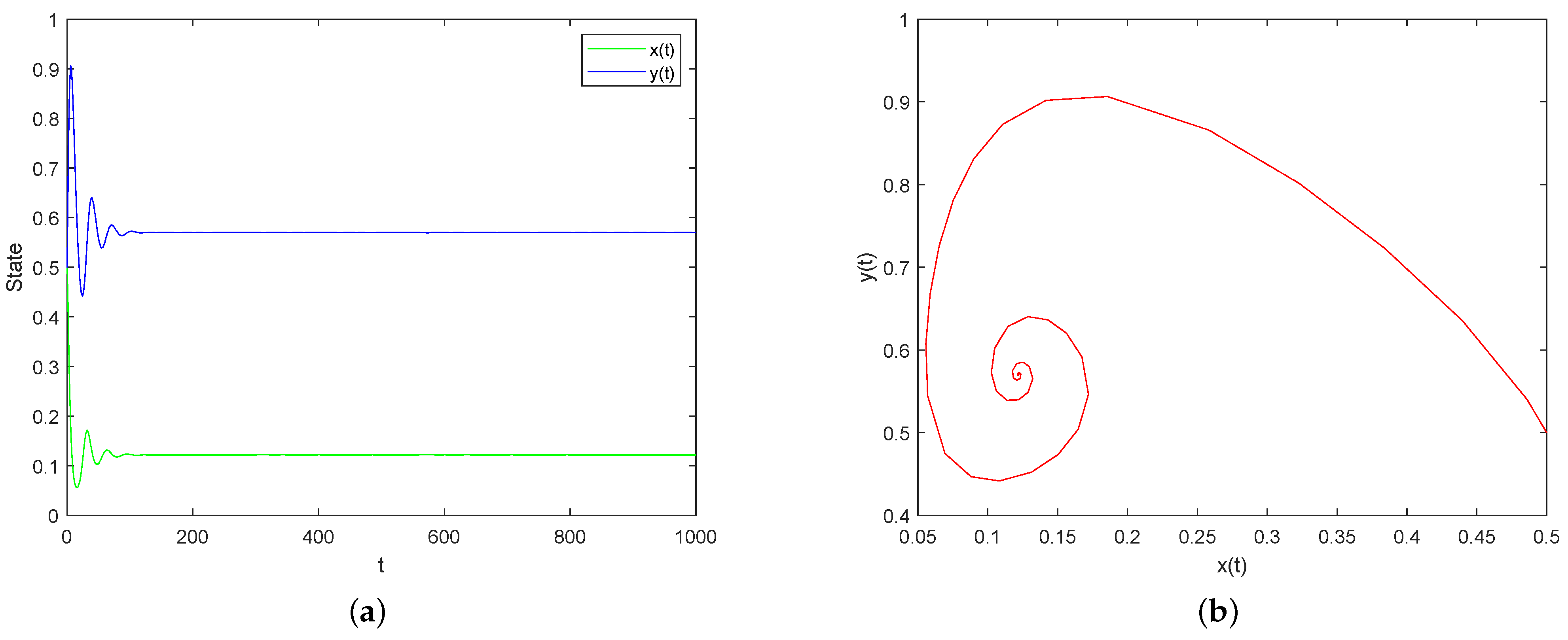
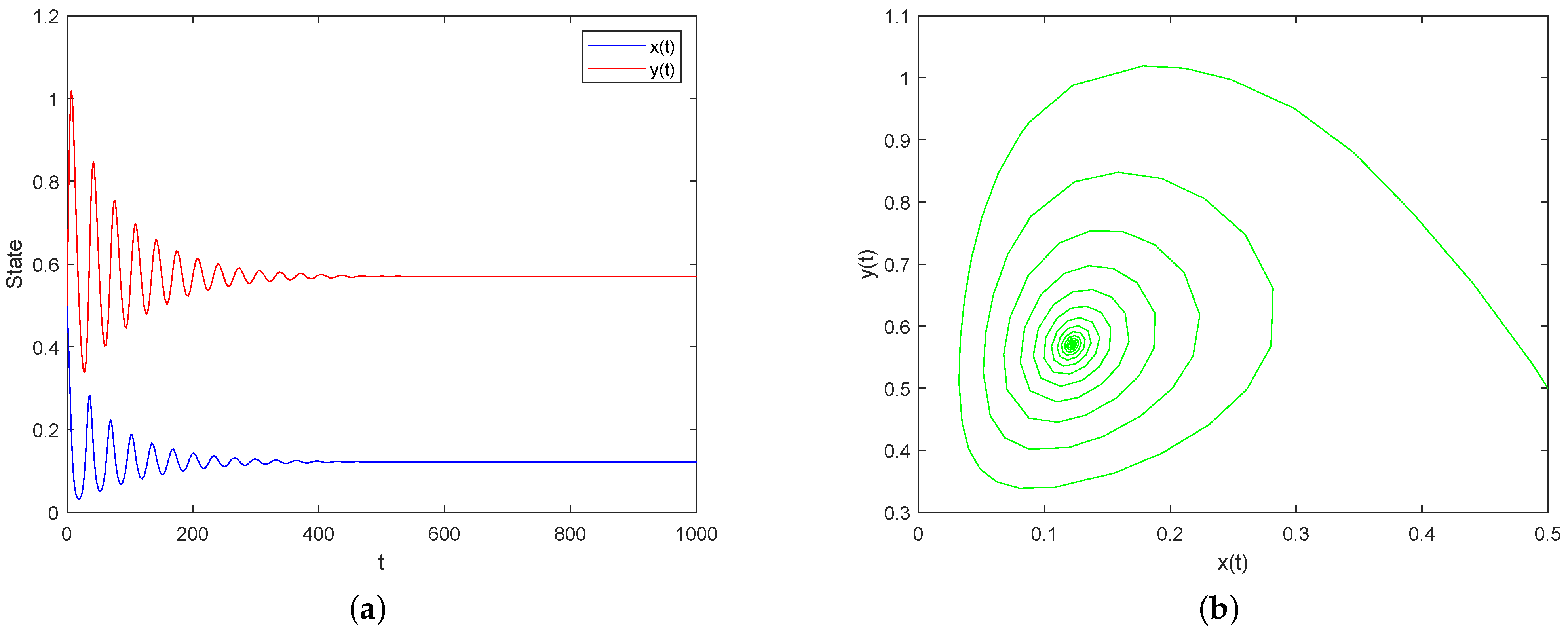
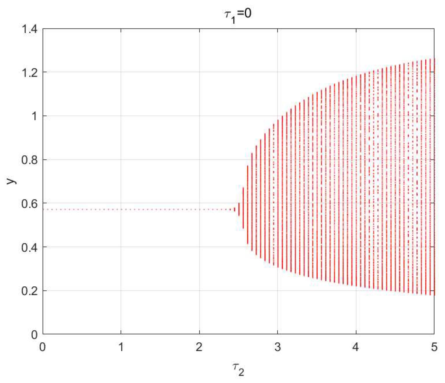
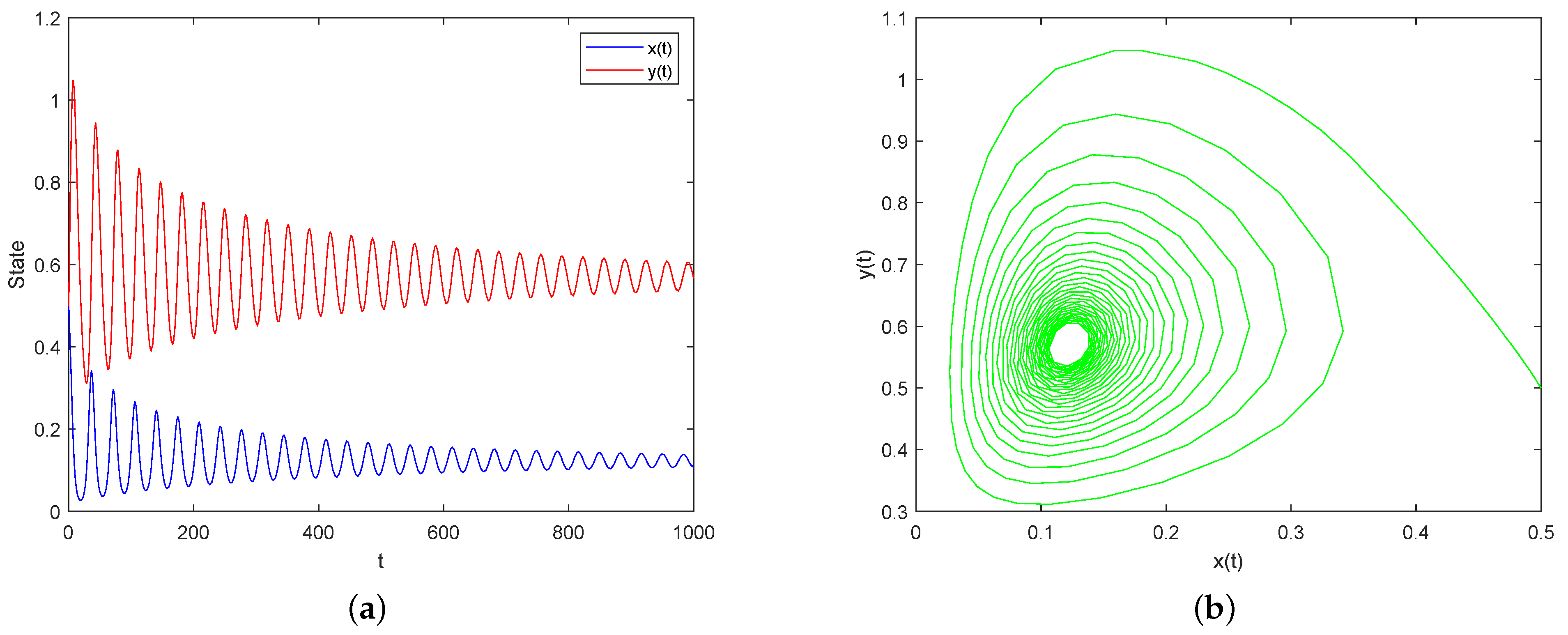
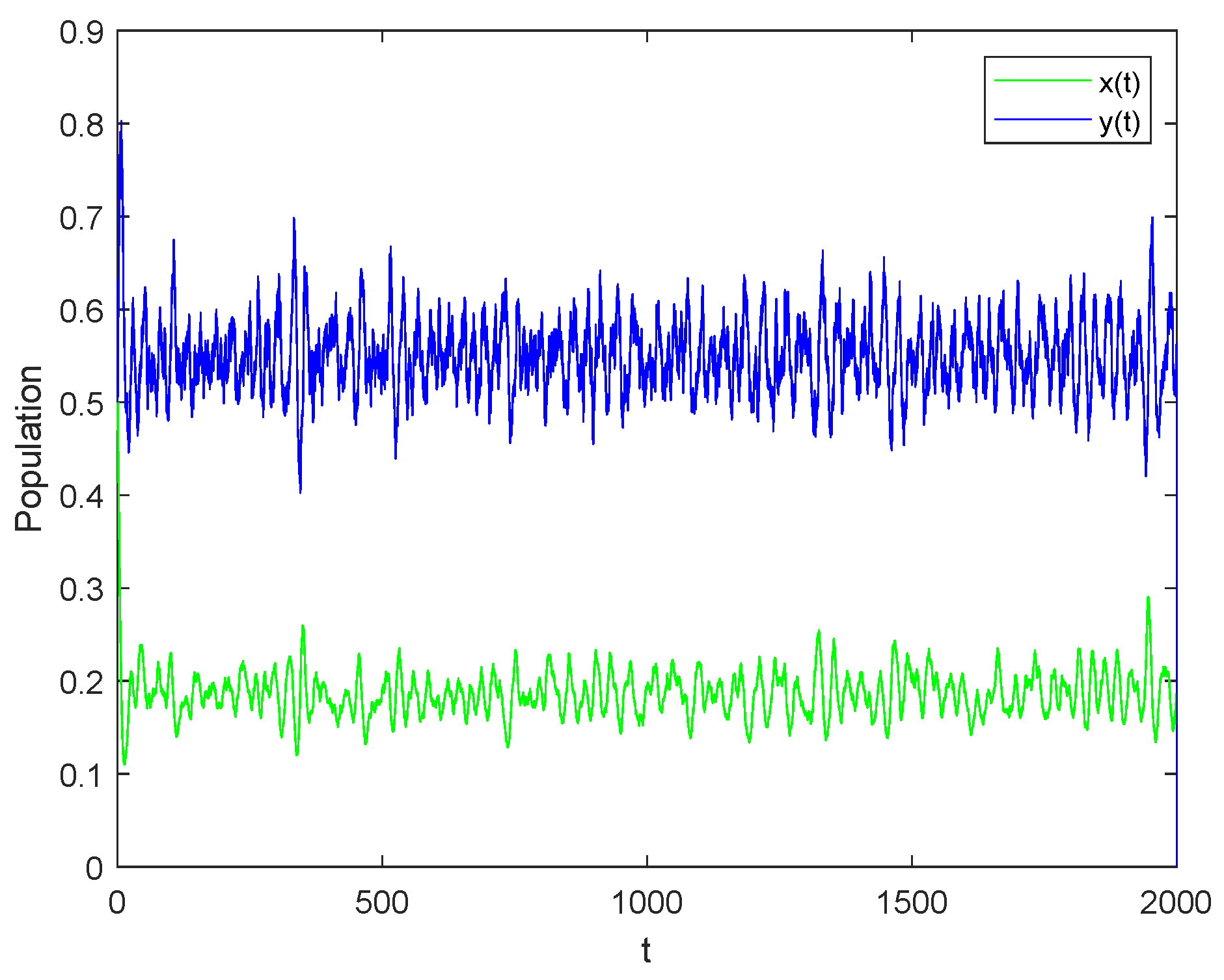
5. Numerical Simulations

In this section, as a general method in stochastic differential equations, we validate our mathematical findings by performing numerical simulations using Milstein’s high-order method [30] and MATLAB 2019a, that is, as proven in the previous sections. We select the following parameters:

$$\begin{array}{c}\hfill f=1.5,p=4,a=4.8,b=5,c=2.1,\mu =1.2,d=0.1,h=0.01,k=0.9,\alpha =0.6,\end{array}$$

(32)

and take the initial data $x\left(0\right)=0.5,y\left(0\right)=0.5$. For the parameters (32), the system (1) has three equilibrium points, which are the trivial equilibrium point $E_0(0,0)$, the free equilibrium point $E_1(1.5,0)$, and the coexistence equilibrium point $E^{*}(x^{*},y^{*})=(0.1219,0.5702)$. By Theorem (3), $E_0$ is always unstable. Furthermore, the existence of $E^{*}$ confirms that $E_2$ is unstable for any ${\tau }_1\ge 0$ and ${\tau }_2\ge 0$.

Case I: Assume ${\tau }_1=0$ and ${\tau }_2=0$ and keep other parameters the same as (32). By simple calculation, $\frac{ap{y}^{*}}{\alpha {(a{x}^{*}+b{y}^{*}+c)}^2}-1=-0.4047<0$. Then, the condition of Theorem 5 is satisfied, which implies that $E^{*}$ is locally asymptotically stable, as shown in Figure 1.

Case II: Assume ${\tau }_2=0$ and slowly increase the value of ${\tau }_1$. Leave the other parameters remain (32) unchanged. By virtue of Theorem 6, we can obtain the critical value of ${\tau }_1={\tau }_1^{*}=4.5923$. When ${\tau }_1=3.5<{\tau }_1^{*}$, the system (1) is locally asymptotically stable (as shown in Figure 2) and unstable for ${\tau }_1=5>{\tau }_1^{*}$. Furthermore, the occurrence of oscillation behavior and limit cycle is illustrated by Figure 3. Furthermore, the system (1) undergoes a Hopf bifurcation at ${\tau }_1={\tau }_1^{*}$ as shown in Figure 4.

Case III: Assume ${\tau }_1=0$ and gradually increase the value of ${\tau }_2$, keeping other parameters remaining in (32) unchanged. After numerical calculation $R_4=-0.0015<0$, according to Theorem 7, we can obtain the critical value of ${\tau }_2={\tau }_2^{*}=2.3941$. When ${\tau }_2=1.5<{\tau }_2^{*}$, the system (1) is locally asymptotically stable as shown in Figure 5 and unstable for ${\tau }_2=2.5>{\tau }_2^{*}$, which is illustrated by Figure 6. Furthermore, the system (1) experiences a Hopf bifurcation at ${\tau }_2={\tau }_2^{*}$ (as shown in Figure 7).

Case IV: We take a fixed ${\tau }_1=3.5\in (0,{\tau }_1^{*})=(0,4.5923)$ and vary the parameter ${\tau }_2$ while keeping other parameters the same as in (32). From Theorem 8, we can see that the critical value of ${\tau }_2={\tilde{\tau }}_2^{*}=0.4830$. When ${\tau }_2=0.2<{\tilde{\tau }}_2^{*}$, the system (1) is locally asymptotically stable as shown in Figure 8 and unstable for ${\tau }_2=0.5>{\tilde{\tau }}_2^{*}$, which is illustrated by Figure 9. Figure 10 reveals that a Hopf bifurcation occurs at ${\tau }_2={\tilde{\tau }}_2^{*}$.

For stochastic delay systems (3), according to Theorem 10, it is random and ultimately bounded. Figure 11 confirms our results.

6. Conclusions

In this paper, we mainly investigate a predator–prey model with Beddington–DeAngelis functional response and fear by predator. At the same time, because predator–prey interactions do not occur immediately, we introduced the fear delay and the pregnancy delay to make the model more natural.

First, we prove the positivity and boundedness of system (1). Then, we discuss the existence criterion and local stability of equilibrium point, and find that the existence of $E^{*}$ ensures that $E_1$ is unstable. Finally, the existence of a Hopf bifurcation with the fear delay ${\tau }_1$ and the pregnancy delay ${\tau }_2$ as the bifurcation parameter is studied, and the critical values of the bifurcation parameters are derived in several possible cases. We find the relationship between local stability and critical bifurcation value of the system (1). When the delay is less than the critical bifurcation value, both prey and predator oscillate periodically for a finite time and then reach equilibrium. When the delay exceeds the critical bifurcation value, Hopf bifurcation occurs in system (1), and periodic oscillation and limit cycle are generated. At this point, the system (1) switches from a stable state to an unstable state. Numerical simulations confirm our theoretical findings. Furthermore, for stochastic delay system (3), we study the unique existence of the global positive solution and explore the stochastic ultimate boundedness.

In future studies, we can generalize the model (1) to a multi-population model and introduce prey refuge to investigate its impact on the stability and persistence of population dynamics. In the meantime, it may be possible to study prey refuge as a Hopf bifurcation parameter. We leave these interesting questions for further study.

References

1. Sahoo, D.; Samanta, G.P. Impact of fear effect in a two prey-one predator system with switching behaviour in predation. Differ. Equ. Dyn. Syst. 2021, 1–23. [Google Scholar] [CrossRef]
2. Mondal, B.; Sarkar, S.; Ghosh, U. Complex dynamics of a generalist predator–prey model with hunting cooperation in predator. Eur. Phys. J. Plus 2022, 137, 43. [Google Scholar] [CrossRef]
3. Pal, S.; Majhi, S.; Mandal, S.; Pal, N. Role of fear in a predator–prey model with Beddington–DeAngelis functional response. Z. FüR Nat. A 2019, 74, 581–595. [Google Scholar] [CrossRef]
4. Huang, G.; Ma, W.; Takeuchi, Y. Global analysis for delay virus dynamics model with Beddington–DeAngelis functional response. Appl. Math. Lett. 2011, 24, 1199–1203. [Google Scholar] [CrossRef] [Green Version]
5. Alam, S. Risk of disease-selective predation in an infected prey-predator system. J. Biol. Syst. 2009, 17, 111–124. [Google Scholar] [CrossRef]
6. Roy, J.; Alam, S. Dynamics of an autonomous food chain model and existence of global attractor of the associated non-autonomous system. Int. J. Biomath. 2019, 12, 1950082. [Google Scholar] [CrossRef]
7. Zanette, L.Y.; White, A.F.; Allen, M.C.; Clinchy, M. Perceived predation risk reduces the number of offspring songbirds produce per year. Science 2011, 334, 1398–1401. [Google Scholar] [CrossRef]
8. Creel, S.; Christianson, D.; Liley, S.; Winnie, J.A., Jr. Predation risk affects reproductive physiology and demography of elk. Science 2007, 315, 960. [Google Scholar] [CrossRef] [PubMed] [Green Version]
9. Eggers, S.; Griesser, M.; Nystr, M.; Ekman, J. Predation risk induces changes in nest-site selection and clutch size in the Siberian jay. PRoceedings R. Soc. B Biol. Sci. 2006, 273, 701–706. [Google Scholar] [CrossRef] [Green Version]
10. Orrock, J.L.; Fletcher, R.J., Jr. An island-wide predator manipulation reveals immediate and long-lasting matching of risk by prey. Proc. R. Soc. B Biol. Sci. 2014, 281, 20140391. [Google Scholar] [CrossRef]
11. Sheriff, M.J.; Krebs, C.J.; Boonstra, R. The sensitive hare: Sublethal effects of predator stress on reproduction in snowshoe hares. J. Anim. Ecol. 2009, 78, 1249–1258. [Google Scholar] [CrossRef] [PubMed]
12. Creel, S.; Christianson, D. Relationships between direct predation and risk effects. Trends Ecol. Evol. 2008, 23, 194–201. [Google Scholar] [CrossRef] [PubMed]
13. Lima, S.L. Predators and the breeding bird: Behavioral and reproductive flexibility under the risk of predation. Biol. Rev. 2009, 84, 485–513. [Google Scholar] [CrossRef] [PubMed]
14. Mondal, S.; Maiti, A.; Samanta, G.P. Effects of fear and additional food in a delayed predator–prey model. Biophys. Rev. Lett. 2018, 13, 157–177. [Google Scholar] [CrossRef]
15. Shao, Y. Global stability of a delayed predator–prey system with fear and Holling-type II functional response in deterministic and stochastic environments. Math. Comput. Simul. 2022, 200, 65–77. [Google Scholar] [CrossRef]
16. Xia, Y.; Yuan, S. Survival analysis of a stochastic predator–prey model with prey refuge and fear effect. J. Biol. Dyn. 2020, 14, 871–892. [Google Scholar] [CrossRef]
17. Liu, S.; Beretta, E.; Breda, D. Predator–prey model of Beddington–DeAngelis type with maturation and gestation delays. Nonlinear Anal. Real World Appl. 2010, 11, 4072–4091. [Google Scholar] [CrossRef]
18. Bhattacharyyai, A.; Pal, A.K. Complex dynamics of delay induced two-prey one-predator model with Beddington-DeAngelis response function. Nonlinear Stud. 2021, 28. [Google Scholar]
19. Li, J.; Liu, X.; Wei, C. The impact of fear factor and self-defence on the dynamics of predator-prey model with digestion delay. Math. Biosci. Eng. 2021, 18, 5478–5504. [Google Scholar] [CrossRef]
20. Djilali, S.; Cattani, C.; Guin, L.N. Delayed predator–prey model with prey social behavior. Eur. Phys. J. Plus 2021, 136, 940. [Google Scholar] [CrossRef]
21. Shu, H.; Hu, X.; Wang, L.; Watmough, J. Delay induced stability switch, multitype bistability and chaos in an intraguild predation model. J. Math. Biol. 2015, 71, 1269–1298. [Google Scholar] [CrossRef]
22. Yuan, J.; Zhao, L.; Huang, C.; Xiao, M. Stability and bifurcation analysis of a fractional predator–prey model involving two nonidentical delays. Math. Comput. Simul. 2021, 181, 562–580. [Google Scholar] [CrossRef]
23. Kong, W.; Shao, Y. The long time behavior of equilibrium status of a predator-prey system with delayed fear in deterministic and stochastic scenarios. J. Math. 2022, 2022, 3214358. [Google Scholar] [CrossRef]
24. Pay, P.; Samanta, S.; Pal, N.; Chattopadhyay, J. Delay induced multiple stability switch and chaos in a predator–prey model with fear effect. Math. Comput. Simul. 2020, 172, 134–158. [Google Scholar]
25. Kumar, A.; Dubey, B. Modeling the effect of fear in a prey–predator system with prey refuge and gestation delay. Int. J. Bifurc. Chaos 2019, 29, 1950195. [Google Scholar] [CrossRef]
26. Roy, J.; Alam, S. Fear factor in a prey–predator system in deterministic and stochastic environment. Phys. A Stat. Mech. Its Appl. 2020, 541, 123359. [Google Scholar] [CrossRef]
27. Yang, X.; Chen, L.; Chen, J. Permanence and positive periodic solution for the single-species nonautonomous delay diffusive models. Comput. Math. Appl. 1996, 32, 109–116. [Google Scholar] [CrossRef] [Green Version]
28. Freedman, H.L.; Sree Hari Rao, V. The trade-off between mutual interference and time lags in predator-prey systems. Bull. Math. Biol. 1983, 45, 991–1004. [Google Scholar] [CrossRef]
29. Peng, S.; Zhu, X. Necessary and sufficient condition for comparison theorem of 1-dimensional stochastic differential equations. Stoch. Process. Their Appl. 2006, 116, 370–380. [Google Scholar] [CrossRef] [Green Version]
30. Higham, D.J. An algorithmic introduction to numerical simulation of stochastic differential equations. SIAM Rev. 2001, 43, 525–546. [Google Scholar] [CrossRef]
Figure 1. (a) Time series and (b) phase portrait of E * for system (1) when τ 1 = 0 and τ 2 = 0 . Other parameters are the same as in (32).
Axioms 12 00073 g001
Figure 2. (a) Time series and (b) phase portrait of E * for system (1) when τ 1 = 3.5 and τ 2 = 0 . Other parameters are the same as in (32).
Axioms 12 00073 g002
Figure 3. (a) Time series and (b) phase portrait of E * for system (1) when τ 1 = 5 and τ 2 = 0 . Other parameters are same as in (32).
Axioms 12 00073 g003
Figure 4. The Hopf bifurcation diagram of (1) for τ 1 and τ 2 = 0 .
Axioms 12 00073 g004
Figure 5. (a) Time series and (b) phase portrait of E * for system (1) when τ 2 = 1.5 and τ 1 = 0 . Other parameters are the same as in (32).
Axioms 12 00073 g005
Figure 6. (a) Time series and (b) phase portrait of E * for system (1) when τ 2 = 2.5 and τ 1 = 0 . Other parameters are the same as in (32).
Axioms 12 00073 g006
Figure 7. The Hopf bifurcation diagram of (1) for τ 2 and τ 1 = 0 .
Axioms 12 00073 g007
Figure 8. (a) Time series and (b) phase portrait of E * for system (1) when τ 1 = 3.5 and τ 2 = 0.2 . Other parameters are the same as in (32).
Axioms 12 00073 g008
Figure 9. (a) Time series and (b) phase portrait of E * for system (1) when τ 1 = 3.5 and τ 2 = 0.5 . Other parameters are the same as in (32).
Axioms 12 00073 g009
Figure 10. The Hopf bifurcation diagram of (1) for τ 2 and τ 1 = 3.5 .
Axioms 12 00073 g010
Figure 11. Dynamical behaviors of (3). The parameters are taken as (32) and σ 1 = 0.03 , σ 2 = 0.03 .
Axioms 12 00073 g011
Disclaimer/Publisher’s Note: The statements, opinions and data contained in all publications are solely those of the individual author(s) and contributor(s) and not of MDPI and/or the editor(s). MDPI and/or the editor(s) disclaim responsibility for any injury to people or property resulting from any ideas, methods, instructions or products referred to in the content.